
15
Mapping the geographic distribution of names
The goal of this exercise is to collect data on the geographic distribution of surnames in Germany. Such maps are a popular visualization in genealogical and onomastic research, that is, research on names and their origins (Barratt 2008; Christian 2012; Osborn 2012). It has been shown that in spite of increased labor mobility in the last decades, surnames that were bound to a certain regional context continue to retain their geographic strongholds (Barrai et al. 2001; Fox and Lasker 1983; Yasuda et al. 1974). Apart from their scientific value, name maps have a more general appeal for those who are interested in the roots of their namesakes. Plus, they visualize the data in one of the most beautiful and insightful ways—geographic maps.
In this chapter, we briefly introduce the visualization of geographic data in R. This can be a difficult task, and if your data do not match the specifications of the data treated in this chapter, we recommend a look at Kahle and Wickham (2013) and Bivand et al. (2013b) for more advanced visualization tools of spatial data with R. In order to acquire the necessary data, we rely on the online directory of a German phone book provider (www.dastelefonbuch.de). As a showcase, we visualize the geographical distribution of a set of surnames in Germany. The goal is to write a program that can easily be fed with any surname to produce a surname map with a single function call. Further, the call should return a data frame that contains all of the scraped observations for further analysis.
The case study serves another purpose: It is not a storybook example of web scraping but shows some of the pitfalls that may occur in reality—and how to deal with them. The case study thus illustrates that textbook theory does not always match up with reality. Among the problems we have to tackle are (a) incomplete and unsystematic data, (b) data that belong together but are dispersed in the HTML tree, (c) limited “hits per page” functionality, and (d) undocumented URL parameters.
15.1 Developing a data collection strategy
Before diving into the online phone book, we begin with some thoughts on the kind of information we want to collect and whether a phone book is an appropriate source for such information. The goal is to gain insight into the current distribution of surnames. The distribution is defined by the universe of surnames in the German population, that is, around 80 million people. We want to collect data for descriptive as well as for secondary analyses. The ideal source would provide a complete and up-to-date list of surnames of all inhabitants, linked with precise geographic identifiers. Such a list would raise severe privacy concerns.
By virtue of purpose, phone directories are open data sources. They provide information on names and residencies, so they are a candidate to approximate the true distributions of surnames. In terms of data quality, however, we have to ask ourselves: Are phone directories a reliable and valid source? There is good reason to believe they are: First, they are updated at least annually. Second, geographic identifiers like streets and zip codes are usually precise enough to assess people's locations within a circle of less than 20 km. The fact that phone books provide such accurate geographical identifiers is actually the crucial property of the data source in this exercise. It is difficult to come up with a freely available alternative.
On the downside, we have to be aware of the phone book's limitations. First, not everybody has a phone and not every phone is listed in the phone directory. This problem has aggravated with the proliferation of mobile phones. Second, phone books occasionally contain duplicates. Using zip codes as geographic identifiers adds some noise to the data, but this inaccuracy is negligible. After all, we are interested in the big picture, not in pinpointing names at the street level.
Regarding alternative data sources, there are several websites which provide ready-made distribution maps, often based on phone book entries as well.1 However, these pages usually only offer aggregate statistics or remain vague about the source of the reported maps. The same is true for commercial software that is frequently offered on these sites. Therefore, we rely on online phone directories and produce our own maps.
In order to achieve the goals, we pursue the following strategies:
- Identify an online phone directory that provides the information we need.
- Become familiar with the page structure and choose an extraction procedure.
- Apply the procedure: retrieve data, extract information, cleanse data, and document unforeseen problems that occur during the coding
- Visualize and analyze the data.
- Generalize the scraping task.
Regarding our example, we have done some research on available online phone directories. There are basically two major providers in Germany, www.dastelefonbuch.de and www.dasoertliche.de. Comparing the number of hits for a sample set of names, the results are almost equivalent, so both providers seem to work with similar databases. The display of hits is different, however. www.dastelefonbuch.de allows accessing a maximum of 2000 hits per query and the number of hits per request can be adapted. Conversely, www.dasoertliche.de offers 10,000 hits at most that are are displayed in bundles of 20s. As we prefer to minimize the number of requests for reasons of efficiency and scraping etiquette, we decide to use www.dastelefonbuch.de as primary source of data for the exercise.
15.2 Website inspection
We start with a look at the robots.txt to check whether accessing the page's content via automated methods is accepted at all (see Section 9.3.3). We find that some bots are indeed robota non grata (e.g., the Googlebot-Image and the trovitBot bot; see Figure 15.1). For other undefined bots, some directories are disallowed, for example, /scripts/ or /styles/. The root path is not prohibited, so we can direct small automated requests to the site with a clear conscience. The bottom of the file reveals some interesting XML files. Accessing these links, we find large compressed XML files that apparently contain information on surnames in all cities. This is potentially a powerful data source, as it might lead to the universe of available surnames in the page's database. We do not make use of the data, however, as it is not immediately obvious how such a list could be used for our specific purpose.
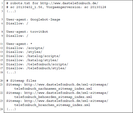
Figure 15.1 Excerpt from the robots.txt file on www.dastelefonbuch.de
We continue with a closer inspection of the page's functionality and architecture. In the simple search mode, we can specify two parameters—whom to search for (“Wer/Was”) and where (“Wo”). Let us start with a sample request. We search for entries with the surname “Feuerstein.”2 In the left column, the total number of hits are reported (837), 149 of which are businesses and 688 of which are private entries. We are only interested in private entries and have already selected this subsample of hits. The hits themselves are listed in the middle column of the page. Surname and, if available, first name is reported in an entry's first row, the address in the second. Some entries do not provide any address. In the rightmost column on the page, the hits are already displayed on a map. This is the information we are looking for, but it seems more convenient to scrape the data from the list of hits rather than from the JavaScript-based map.3 We also observe that the URL has changed after passing the request to the server. In its complete form, it looks as follows:
http://www3.dastelefonbuch.de/?bi=76&kw=Feuerstein&cmd=search&seed=
1010762549&ort_ok=1&vert_ok=1&buab=622100&mergerid=A43F7DB343E7F461D
5506CA8A7DBB734&mdest=sec1.www1%2Csec2.www2%2Csec3.www3%2Csec4.www4
&recfrom=&ao1=1&ao2=0&sp=51&aktion=105
Evidently, passing the input form to the server has automatically added a set of parameters, which can be observed in the URL's query string, beginning after the ? sign.4 As we need to set these parameters with our program later on, we have to identify their meaning. Unfortunately, there is no documentation in the page's source code. Therefore, we try to detect their meaning manually by playing around with them and comparing the displayed outputs. We find that the kw parameter contains the keyword we are searching for. Note that URL encoding is required here, that is, we look for M%FCller instead of Müller and so on. cmd=search is the trigger for the search action, ao1=1 means that only private entries are shown. Some of the parameters can be dropped without any changes in the displayed content. By manually specifying some of the search parameters, we identify another useful parameter: reccount defines the number of hits that are shown on the page. We know from search engine requests that this number is usually limited to around 10–50 hits for efficiency reasons. In this case, the options displayed in the browser are 20, 50, and 100 hits per page. However, we can manually specify the value in the URL and set it up to a maximum of 2000 hits. This is very useful, as one single request suffices to scrape all available results. In general, inspecting the URL before and after putting requests to the server often pays off in web scraping practice—and not only for an ad-hoc URL manipulation strategy as proposed in Section 9.1.3. In this case, we can circumvent the need to identify and scrape a large set of sites to download all hits. Having said that, we can now start constructing the web scraper.
15.3 Data retrieval and information extraction
First, we load a couple of packages that are needed for the exercise. Beside the set of usual suspects RCurl, XML, and stringr, we load three additional packages which provide helpful functions for geographical work: maptools (Bivand and Lewin-Koh 2013), rgdal (Bivand et al. 2013a), maps (Brownrigg et al. 2013), and TeachingDemos (Snow 2013).
R> library(RCurl)
R> library(XML)
R> library(stringr)
R> library(maptools)
R> library(rgdal)
R> library(maps)
R> library(TeachingDemos)
We identified the parameters in the URL which tell the server to return a rendered HTML page that meets our requirements. In order to retrieve the results of a search request for the name “Feuerstein,” we use getForm() and specify the URL parameters in the .params argument.
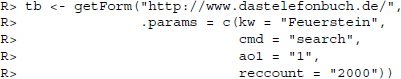
Note that we set the reccount parameter to the maximum value of 2000 to ensure that all hits that are retrievable with one request are actually captured. If the number of hits is greater, we just get the first 2000. We will discuss this shortcoming of our method further below. The returned content is stored in the object tb which we write to the file phonebook_ feuerstein.html on our local drive.
R> dir.create(”phonebook_feuerstein”)
R> write(tb, file = ”phonebook_feuerstein/phonebook_feuerstein.html”)
We can now work with the offline data and do not have to bother the server again—the screen scraping part in the narrow sense of the word is finished. In order to be able to access the information in the document by exploiting the DOM, we parse it with htmlParse() and ensure that the original UTF-8 encoding is retained.
![]()
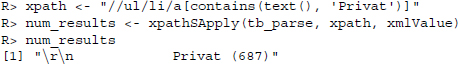
We can start extracting the entries. As a first benchmark, we want to extract the total number of results in order to check whether we are able to scrape all entries or only a subset. The number is stored in the left column as “Privat (687).” In order to retrieve this number from the HTML file, we start with an XPath query. We locate the relevant line in the HTML code—it is stored in an unordered list of anchors. We retrieve the anchor within that list that contains the text pattern “Privat.”
In the next step, we extract the sequence of digits within the string using a simple regular expression.
R> num_results <- as.numeric(str_extract(num_results, ”[[:digit:]]+”))
R> num_results
[1] 687
As so often in web scraping, there is more than one way of doing it. We could replace the XPath/regex query with a pure regex approach, eventually leading to the same result.
We now come to the crucial part of the matter, the extraction of names and geographic information. In order to locate the information in the tree, we inspect some of the elements in the list of results. By using the “inspect element” or a similar option in our browser to identify the data in the HTML tree (see Section 6.3), we find that the name is contained in the attribute title of an element <a> which is child of a <div> tag of class name. This position in the tree can easily be generalized by means of an XPath expression.
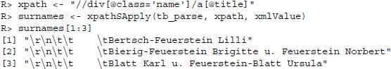
Apart from redundant carriage return and line feed symbols which have to be removed in the data-cleansing step, this seems to have worked well. Extracting the zip codes for geographic localization is also simple. They are stored in the <span> elements with the attribute itemprop=”postal-code”. Accordingly, we write
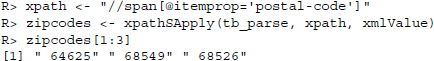
When trying to match the names and the zip code vector, we realize that fetching both pieces of information separately was not a good idea. The vectors have different lengths.
R> length(surnames)
[1] 687
R> length(zipcodes)
[1] 642
A total of 45 zip codes seem to be missing. A closer look at the entries in the HTML file reveals that some entries lack an address and therefore a zip code. Unfortunately, the <span> element with the attribute itemprop=”postal-code” is also missing in these cases. If we were only interested in the location of hits, we could drop the names and just extract the zip codes. To keep names and zip codes together for further analyses, however, we have to adapt the extraction function.
In Section 4.2.2 we have encountered a tool that is of great help for this problem—XPath axes. XPath axes help express the relations between nodes in a family tree analogy. This means that they can be used to condition a selection on attributes of related nodes. This is precisely what we need to extract names and zip codes that belong together. As names without zip codes are meaningless for locating observations on a map, we want to extract only those names for which a zip code is available. The necessary XPath expression is a bit more complicated.
R> xpath <- ”//span[@itemprop=‘postal-code‘]/ancestor::div[@class=‘
popupMenu‘]/preceding-sibling::div[@class=‘name‘]”
R> names_vec <- xpathSApply(tb_parse, xpath, xmlValue)
Let us consider this call step by step from back to front. What we are looking for is a <div> object of class name. It is the preceding-sibling of a <div> object of class popupMenu. This <div> element is the ancestor of a span element with attribute itemprop=”postal-code”. Applying this XPath query to the parsed document with xpathSApply() returns a vector of names which are linked to a zip code. By inverting the XPath expression, we extract the zip codes as well.
R> xpath <- ”//div[@class=‘name‘]/following-sibling::div[@class=‘
popupMenu‘]//span[@itemprop=‘postal-code‘]”
R> zipcodes_vec <- xpathSApply(tb_parse, xpath, xmlValue)
We compare the lengths of both vectors and find that they are now of equal length.
R> length(names_vec)
[1] 642
R> length(zipcodes_vec)
[1] 642
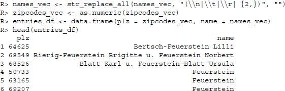
In a last step, we remove the carriage returns ( ), line feeds ( ), horizontal tabs ( ), and empty spaces in the names vector, coerce the zip code vector to be numeric, and merge both variables in a data frame.
15.4 Mapping names
Regarding the scraping strategy outlined in the first section, we have just completed step 3 after having retrieved the data, extracted the information, and cleansed the data. The next step is to plot the scraped observations on a map. To do so, we have to (1) match geo-coordinates to the scraped zip codes and (2) add them to a map.
After some research on the Web, we find a dataset that links zip codes (“Postleitzahlen,” PLZ) and geographic coordinates. It is part of the OpenGeoDB project (http://opengeodb .org/wiki/OpenGeoDB) and freely available. We save the file to our local drive and load it into R.
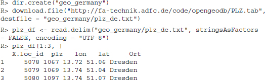
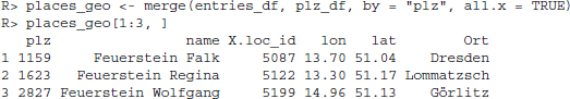
We can easily merge the information to the entries_df data frame using the joint identifying variable plz.
In order to enrich the map with administrative boundaries, we rely on data from the Global Administrative Areas database (GADM; www.gadm.org). It offers geographic data for a multitude of countries in various file formats. The data's coordinate reference system is latitude/longitude and the WGS84 datum, which matches nicely with the coordinates from the zip code data frame.5 We download the zip file containing shapefile data for Germany and unzip it in a subdirectory:
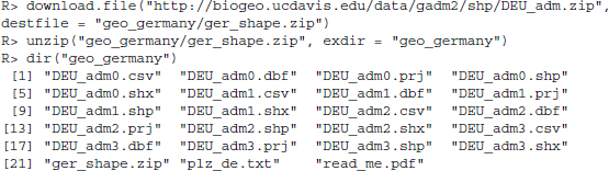
The downloaded archive provides a set of files. A shapefile actually consists of at least three files: The .shp file contains geographic data, the .dbf file contains attribute data attached to geographic objects, and the .shx file contains an index for the geographic data. The .prj files in the folder are optional and contain information about the shapefile's projection format. Altogether, there are four shapefiles in the archive for different levels of administrative boundaries. Using the maptools package (Bivand and Lewin-Koh 2013), we import and process shapefile data in R. The readShapePoly() function converts the shapefile into an object of class SpatialPolygonsDataFrame. It contains both vector data for the administrative units (i.e., polygons) and substantive data linked to these polygons (therefore “DataFrame”). We import two shapefiles: the highest-level boundary, Germany's national border, and the second highest-level boundaries, the federal states. Additionally, we declare the data to be projected according to the coordinate reference system WGS84 with the CRS() function and the proj4string argument.
Finally, we transform the coordinates of our entries to a SpatialPoints object that harmonizes with the map data.
R> coords <- SpatialPoints(cbind(places_geo$lon, places_geo$lat))
R> proj4string(coords) <- CRS(”+proj=longlat +ellps=WGS84 +datum=WGS84”)
In order to get a better intuition of where people are located, we add the location of Germany's biggest cities as well. The maps package (Brownrigg et al. 2013) is extraordinarily useful for this purpose, as it contains a list of all cities around the world, including their coordinates. We extract the German cities with a population greater than 450,000—an arbitrary value that results in a reasonable number of cities displayed—and add two more cities that are located in interesting areas.
We compose the map sequentially by adding layer after layer. First, we plot the national border, then we add the federal states boundaries. The scraped locations of the “Feuersteins” are added with the points() function, as well as the cities’ locations. Finally, we add the cities’ labels.
R> plot(map_germany)
R> plot(map_germany_laender, add = T)
R> points(coords$coords.x1, coords$coords.x2, pch = 20)
R> points(coords_cities, col = ”black”, , bg = ”grey”, pch = 23)
R> text(cities_ger$long, cities_ger$lat, labels = cities_ger$name, pos = 4)
The result is provided in Figure 15.2. The distribution of hits reveals some interesting facts. The largest cluster of Feuersteins lives in the southwestern part of Germany, in the area near Mannheim.
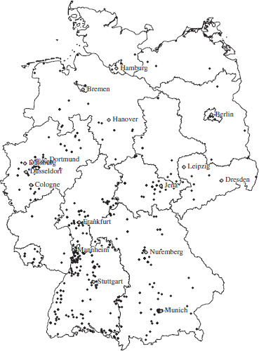
Figure 15.2 Geographic distribution of “Feuersteins”
15.5 Automating the process
Crafting maps from scraped surnames is an example of a task that is likely to be repeated over and over again, with only slight modifications. To round off the exercise, we develop a set of functions which generalize the scraping, parsing, and mapping from above and offer some useful options to adapt the process (see Section 11.3). In our case, the information for one name rarely changes over time. It is thus of less interest to repeat the task for one surname. Instead, we want to be able to quickly produce data and maps for any name.
We decide to split the procedure into three functions: a scraping function, a parsing and data cleansing function, and a mapping function. While on the one side this means that we have to call three functions to create a map, these functions are easier to debug and adapt. The code in Figures 15.3, 15.4, and 15.5 displays the result of our efforts. It is the condensed version of the code snippets from above, enriched with some useful arguments for the function sets namesScrape(), namesParse(), and namesPlot().
Usually, what distinguishes functions from ordinary code is that they (1) generalize a task and (2) offer flexibility in the form of arguments. It is always the choice of a function author which parameters to keep variable, that is, easily modifiable by the function user, and which parameters to fix. For our functions, we have implemented a set of arguments which is listed in Table 15.1.
Table 15.1 Parameters of phone book scraping functions explained
| Argument | Description |
| phonename | Main argument for namesScrape() and namesParse(); defines the name for which entries should be retrieved |
| geodf | Main argument for namesPlot; specifies data.frame object which stores geographical information (object is usually returned by namesParse()) |
| update.file | Logical value indicating whether the data should be scraped again or if existing data should be used |
| show.map | Logical value indicating whether R should automatically print a map with the located observations |
| save.pdf | Logical value indicating whether R should save the map as pdf |
| minsize.cities | Numerical value setting the minimal size of cities to be included in the plot |
| add.cities | Character values defining names of further cities to be added to the plot |
| print.names | Logical value indicating whether people's names should be plotted |
The choice of arguments is mainly focused on plotting the results. One could easily think of more options for the scraping process. We could allow more than one request at once, explicitly obey the robots.txt,6 or define a User-agent header field. With regards to processing, we could have allowed specifying a directory where data and maps should be saved. For reasons of brevity, we refrain from such fine-tuning work. However, anybody should feel free to adapt and expand the function.
Let us consider the details of the code. In the scraping function namesScrape() (Figure 15.3), phonename is the crucial parameter. We use the tolower() function (see Section 8.1) to achieve a consistent naming of files. Data are stored as follows: Using a call to dir.create(), a directory is created where the HTML file and, if so desired, a PDF version of the graph are stored. Scraping is only performed if the file does not exist. This is checked with the file.exists() function or if the user explicitly requests that the file be updated (option update.file == TRUE). Otherwise, a message referring to the existing file is shown and the function loads the old data.
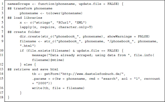
Figure 15.3 Generalized R code to scrape entries from www.dastelefonbuch.de
In the parsing function namesParse() (Figure 15.4), the information extraction process remains the same as above, except that the number of results is reported. The function prints a warning if more than 2000 observations are found. This would mean that not the full sample of observations is captured. Further, first names are extracted from the names vector in a rather simplistic manner by removing the surname. The function returns the data frame which contains geographical and name information for further analysis and/or plotting.
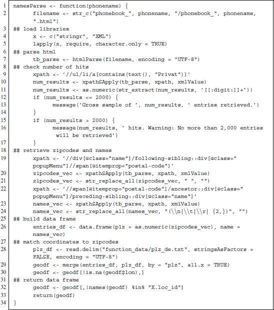
Figure 15.4 Generalized R code to parse entries from www.dastelefonbuch.de
Finally, the plotting function namesPlot() (Figure 15.5) uses the data frame and generates the map as outlined above. The function allows storing the plot locally as a PDF file. We also add the option print.names to print the first names of the observations.
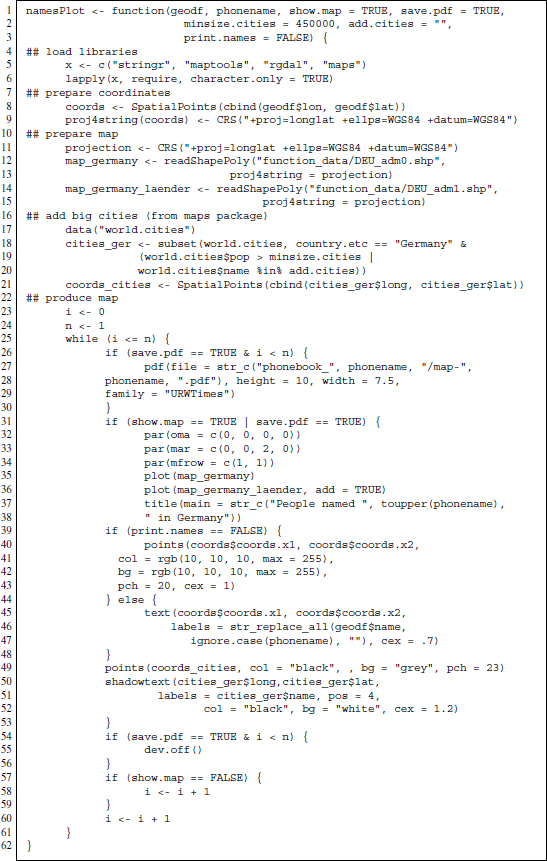
Figure 15.5 Generalized R code to map entries from www.dastelefonbuch.de
We test the functions with a set of specifications. First, we look at the distribution of people named “Gruber,” displaying cities with more than 300,000 inhabitants.
R> namesScrape(”Gruber”)
R> gruber_df <- namesParse(”Gruber”, minsize.cities = 300000)
R> namesPlot(gruber_df, ”Gruber”, save.pdf = FALSE, show.map = FALSE)
Next, we scrape information for people named “Petersen.” We have done this before and force the scraping function to update the file.
R> namesScrape(”Petersen”, update.file = TRUE)
R> petersen_df <- namesParse(”Petersen”)
9605 hits. Warning: No more than 2,000 entries will be retrieved
R> namesPlot(petersen_df, ”Petersen”, save.pdf = FALSE, show.map = FALSE)
Finally, we look at the distribution of the surname “Dimpfl.” We ask the function to plot the surnames.
R> namesScrape(”Dimpfl”)
Data already scraped; using data from 2014-01-16 00:22:03
R> dimpfl_df <- namesParse(”Dimpfl”)
Gross sample of 109 entries retrieved.
R> namesPlot(dimpfl_df, ”Dimpfl”, save.pdf = FALSE, show.map = FALSE, print.names = TRUE)
The output of all three calls is shown in Figure 15.6. We observe that both Gruber and Dimpfl are clustered in the southern part of Germany, whereas Petersens live predominantly in the very north. Note that for the Dimpfls we see first names instead of dots.
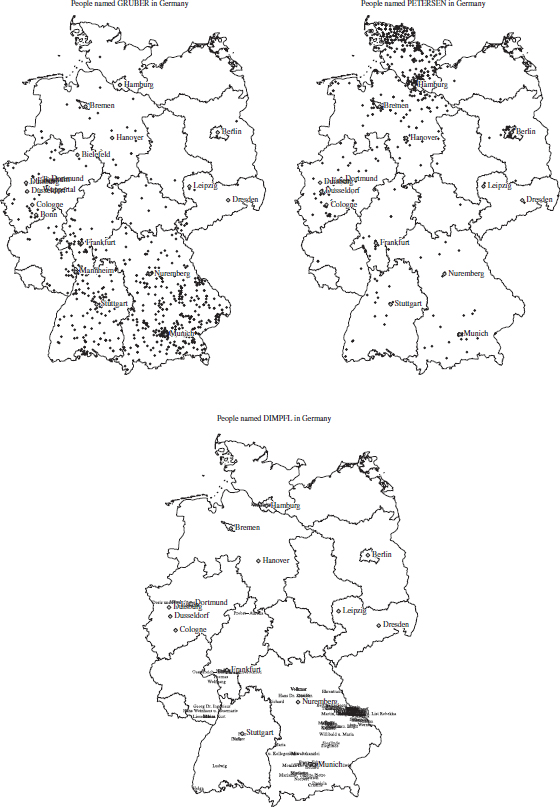
Figure 15.6 Results of three calls of the namesPlot() function
Finally, we reconsider a technical concern of our scraping approach. Recall that in Section 15.2 we noted that the search on www.dastelefonbuch.de also returns a map where the findings are located, which is essentially what we wanted to replicate. We argued that it seems easier to scrape the entries from the list instead of the JavaScript object. Indeed, the inspection of the source code of the page does not reveal any of the hits. But this is what we should expect knowing how dynamic webpages are constructed, that is, by means of AJAX methods (see Chapter 6). Therefore, we use the Web Developer Tools of our browser to identify the source of information which is plotted in the map (see Section 6.3). We find that the script initiates the following GET request:
http://maps.dastelefonbuch.de/DasTelefonbuch/search.html?queryType=
whatOnly&x=1324400.3811369245&y=6699724.7656052755&width=3033021.
2837500004&height=1110477.1474374998&city=&searchTerm=Feuerstein&
shapeName=tb/CA912598AEB53A4D1862D89ACA54C42E_2&minZoomLevel=4&
maxZoomLevel=18&mapPixelWidth=1240&mapPixelHeight=454&order=distance
&maxHits=200
The interesting aspect about this is that this request returns an XML file that contains essentially the same information that we scraped above along with coordinates that locate the hits on the map. One could therefore directly target this file in order to scrape the relevant information. Advantages would be that it is more likely that the XML file's structure remains more stable than the front-end page, making the scraper more robust to changes in the page layout. Second, one could probably skip the step where zip codes and coordinates are matched. However, some parameters in the related URL seem to further restrict the number of returned hits, that is, the zoom level and margins of the plotted area. Further, the structure of the XML document is largely identical with the relevant part of the HTML document we scraped above. This means that the information extraction step should not be expected to be easier with the XML document. Nevertheless, it is always worth looking behind the curtains of dynamically rendered content on webpages, as there may be scenarios in which relevant data can only be scraped this way.
Summary
The code presented in this chapter is only the first step toward a thorough analysis of the distribution of family names. There are several issues of data quality that should be considered when the data are used for scientific purposes. First, there is the limitation of 2000 hits. As the hits are sorted alphabetically, the truncation of the scraped sample is at least not entirely random. Further, the data may contain duplicates or “false positives.” Even if one is not interested in detailed research on the data, there is plenty of room for improvement in the functions. The point representation of hits could be replaced by density maps to better visualize regions where names occur frequently.
More general take-away points of this study are the following. When dealing with dynamic content, it usually pays off to start with a closer look at the source code. One should first get a basic understanding of how parameters in a GET request work, what their limits are, and if there are other ways to retrieve content than to posit requests via the input field. Concerning the use of geo data, the lesson learned is that it is easy to enrich scraped data with geo information once a geographical identifier is available. Mapping such information in R is possible, although not always straightforward. Finally, splitting the necessary tasks into a set of specific functions can be useful and keeps the code manageable.