
17
Analyzing sentiments of product reviews
17.1 Introduction
In the previous chapter, we have assembled several pieces of structured information on a collection of mobile phones from the Amazon website. We have studied how structural features of the phones, most importantly the cost of the phones, are related to consumer ratings. There is one important source of information on the phones we have disregarded so far—the textual consumer ratings. In this chapter, we investigate whether we can make use of the product reviews to estimate the consumer ratings. This might seem a fairly academic exercise, as we have access to more structured information on consumer ratings in the form of stars. Nevertheless, there are numerous circumstances where such structured information on consumer reviews is not available. If we can successfully recover consumer ratings from the mere texts, we have a powerful tool at our disposal to collect consumer sentiment in other applications.
In fact, while structured consumer ratings provide extremely useful feedback for producers, the information in textual reviews can be a lot more detailed. Consider the case of a product review for a mobile phone like we investigate in the present application. Besides reviewing the product itself, consumers make more detailed arguments on the specific product parts that they like or dislike and where they find fault with them. Researchers have made some effort to collect this more specific review (Meng 2012; Mukherjee and Bhattacharyya 2012). In this exercise, our goal is more humble. We investigate whether we are able to estimate the star that a reviewer has given to a product based on the textual review. To do so, we apply the text mining functionality that was introduced in Chapter 10.
We start out in the next section by collecting the reviews from the webpage. We download the files and store them in the previously created database. In the analytical part of the chapter, we first assess the possibility of using a dictionary-based approach to classify the reviews as positive or negative. There are several English dictionaries where researchers have classified terms as signaling either positive or negative sentiment. We check whether the appearance of such signals in the reviews suffices to correctly classify the opinion of the review. In a final step, we use the text mining techniques to label the reviews based on the stars that reviewers have given. We train the algorithms based on half of the data, estimate the second half, and compare our estimates with the star reviews.
17.2 Collecting the data
As a first step we collect the additional data—the textual product reviews—from the Amazon website. We establish a connection to the database that we generated in the previous chapter. The database contains information on the mobile phones, the price and structural features, as well as the average number of stars that were assigned by the users. We download the individual reviews from the website, extract the textual reviews and the associated stars from the source code, and add the information to the database in a new table.
17.2.1 Downloading the files
Let us begin by loading the necessary packages for the operations in this section. For the scraping and extraction tasks, we need stringr, XML, and RCurl. We also load the RSQLite package to get the information in the database from the previous chapter and add the new information to the existing database.
R> library(stringr)
R> library(XML)
R> library(RCurl)
R> library(RSQLite)
We establish a connection to the database using the dbDriver() and dbConnect() functions:
R> sqlite <- dbDriver(”SQLite”)
R> con <- dbConnect(sqlite, ”amazonProductInfo.db”)
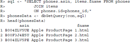
Now we can get data from the database using dbGetQuery(). What we need are the phones’ ASINs (Amazon Standard Identification Numbers) and the name of one of the phones’ product pages. As the information is stored in different tables of the database, we make use of JOIN to merge them, where id from the phones table is matched with phones_id from the items table.
![]()
We create the folder dataReviews via dir.create(), if it does not exist already, to store the downloaded review pages and change the working directory to that folder.
R> if(!file.exists(”dataReviews”)) dir.create(”dataReviews”)
R> setwd(”dataReviews”)
The links to the review pages were part of the product pages we downloaded in the previous case study and were saved in dataFull. Therefore, we read in those files via htmlParse() to be able to extract the review page links.
R> productPageFiles <- str_c(”../dataFull/”, phonesData$fname)
R> productPages <- lapply(productPageFiles, htmlParse)
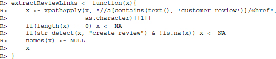
We write a function that collects links to reviews from the phones’ pages. This is done by looking for all <a> nodes that contain the text customer review. We generously discard minor errors, as there are lots more reviews than we can possibly hope to analyze in this application. Specifically, we discard results of length 0 and give them a value of NA and we do the same for links that create new reviews. We also discard the names of the resulting vector and return the results.
We apply our extractReviewLinks() function to all of the parsed phones’ product pages and unlist the result to create a vector of links to the reviews.
R> reviewLinks <- unlist(lapply(productPages, extractReviewLinks))
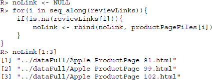
To be able to manually inspect the pages where the review link is missing, we print the names of those product pages to our console. It turns out they are all products where no single review has been written.
Finally, we add the host—http://www.amazon.com—to the links that we collected. We discard the host where it is already part of the link and add it to all the links, except in those cases where we set the entry to NA.
![]()
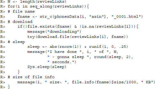
Now we are ready to download the first batch of review pages. We collect the pages by creating a file name that consists of the phones’ ASIN and an index of 0001. If the file does not already exist on the hard drive and the entry is not missing in the link vector we download the file, wrapping the function in a simple try() command. That way, if one download fails it will not stop running the rest of the loop. We add a random waiting period to our downloads to mimic human behavior and avoid being returned an error from amazon.com. We also add two status messages to provide information on the progress of the download.
Again, there is lots more information than we can possibly hope to analyze in this exercise, which is why we generously discard errors. We generate a vector of all downloads that we have collected so far—there should only be review sites that end in the pattern 001.html— and remove pages with sizes of 0.
R> firstPages <- list.files(pattern = ”001.html”)
R> file.remove(firstPages[file.info(firstPages)$size == 0])
R> firstPages <- list.files(pattern = ”001.html”)
All remaining results are parsed and a list of all first review pages is created.
R> HTML <- lapply(firstPages, htmlParse)
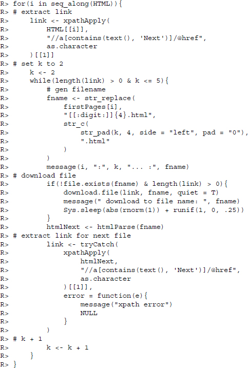
In most cases, there is more than one review page for each mobile phone. For the sake of exposition, we download another four review pages, if available. To do so, we loop through the HTML object from the previous step. We extract the first link to the next review page by looking for an a node that contains the text Next and move one step down the tree to the associated href. While such a link is available and we have not reached the maximum number of review pages k—in our case five, we download another page. We generate a file name, download the link, and store it on our hard drive if it does not already exist. We also parse the downloaded file to look for another Next review page link. This operation is wrapped in a tryCatch() function, in case we fail to find a link.
Finally, we generate a vector of all the files in our dataReviews directory that contain the pattern .html. If all goes as planned, there should not be any file in the directory where this condition is false. We remove files of sizes smaller than 50,000 bytes, as there are presumably errors in these files.
R> tmp <- list.files(pattern = ”.html”)
R> file.remove(tmp[file.info(tmp)$size < 50000])
17.2.2 Information extraction
Having collected the review pages for the phones in our database, we now need to extract the textual reviews and the associated ratings from the pages and add them to the database.
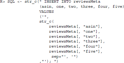
Before extracting the data on individual reviews, we first extract some review meta information on all reviews made for a specific phone. The meta information contains the frequency of reviews giving a phone one up to five stars. The strategy for extracting the meta information is to use readHTMLTable() as the numbers are stored in a table node. To extract only the information we need—the number of reviews per star—we compose a little helper function—getNumbers()—that extracts one up to six digits. This function will be applied to each cell of the table when readHTMLTable() is called.
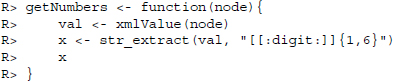
First, we define getNumbers() that extracts the value of a node and extracts digits from it.
We create a vector of all the ASINs of those phones where we have access to customer reviews by listing all the HTML files in the review directory, discarding the indices and duplicate values.
R> FPAsins <- list.files(pattern=”html$”)
R> FPAsins <- unique(str_replace(FPAsins, ”_.+”, ””))
We create an empty data frame to store the meta information.
R> reviewsMeta <- data.frame(asin = FPAsins, one = NA, two = NA,
three = NA, four = NA, five = NA, stringsAsFactors = F)
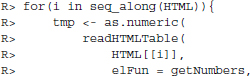
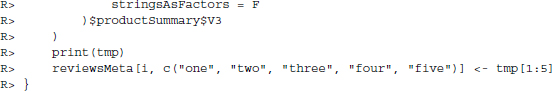
Then, we loop through all our first review pages stored in the list object HTML, extract all tables via readHTMLTable(), and apply getNumbers() to all its elements. From the resulting list of tables, we only keep the table called productSummary and from this only the third variable. The extracted numbers are written into the ith line of reviewsMeta for storage.
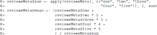
We also compute the sum and the mean consumer rating per phone.
Having extracted the meta information, we now turn to the review specific information. What we would like to have in the resulting data frame are the ASIN, how many stars the reviewer gave the product, how many users found the review helpful and not helpful, the date the review was written, the title of the review, and the text of the review. To store the information, we first create an empty data frame.
R> reviews <- data.frame(asin = NA, stars = 0, helpfulyes = 0,
helpfulno = 0, helpfulsum = 0, date = ””, title = ””, text = ””,
stringsAsFactors = F)
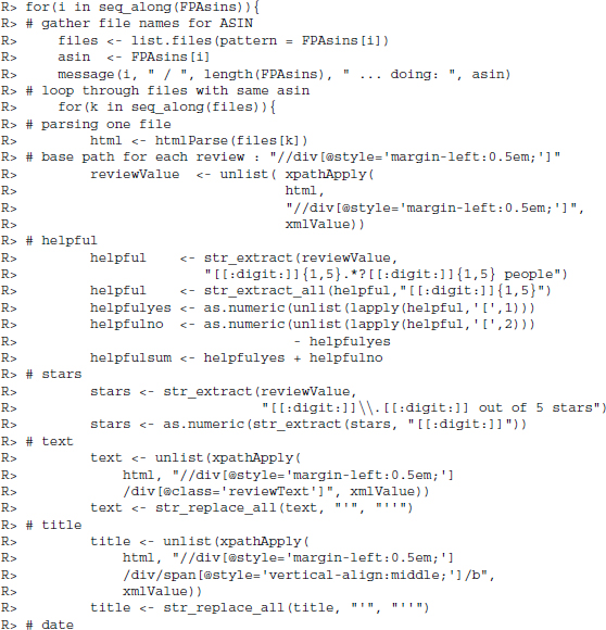
The next block of code might seem a little complicated but it is really only a series of simple steps that is executed for all ASINs and all review pages belonging to the same ASIN. First of all, we use two loops for extracting the data. The outer loop with index i refers to the ASINs. The inner loop with index k refers to the one up to five review pages we collected for that product. The outer loop retrieves the file names of the review pages belonging to that product and stores them in files. It stores the ASIN for these review pages in asin and posts a progress message to the console.
In the inner loop, we first parse one file and store its representation in html. Next, we extract the value of all review nodes in a vector for later extraction of the consumer ratings and supplementary variables. All reviews are enclosed by a div node with style=’margin-left:0.5em;. As this distinctive text pattern is easy to extract with a regular expression, we directly extract the value of the whole node instead of specifying a more elaborate XPath that would need further extraction via regular expressions anyways.
The information whether or not people found the review helpful is always given in the following form. 1 of 1 people found the following review helpful. We make use of this pattern by extracting a string—as short as possible—that starts with one up to five digits and ends with people. We extract all sequences of digits from the substring and use these numbers to fill up the helpful variables—helpfulyes, helpfulno, and helpfulsum.
The consumer rating given to the product also follows a distinct pattern, for example, 5.0 out of 5 stars. To collect this, we extract a substring starting with a digit dot digit and ending with stars and extract the first digit from the substring to get the rating.
The text of the reviews is extracted using XPath again as it has a distinct class—reviewText. We look for a div node with this class and specify that xpathApply should return the value of this node. Note, that both title and text of the reviews might contain single quotation marks that might later on interfere with the SQL statements. Therefore, we replace every single quotation mark by a sequence of two single quotation marks. Most SQL databases will recognize this as a way to escape single quotation marks and store only one single quotation mark.
The title and date are both located in a span node which is a child of a div node, which is a child of another div that encloses all review information. The span’s class is distinct in this subpath and while the title is set in bold—a b node—the date is enclosed by a nobr node. With two calls to xpathApply() we extract the value for each path.
As there are up to 10 reviews per page, all information—helpful variables, consumer rating, text, title, and date—result in vectors. These vectors are combined via cbind() into the matrix tmp and appended via rbind() to the prepared data frame reviews.
Finally, we keep only those lines of reviews where the first line is not NA to get rid of the dummy data we introduced to create the data frame in the first place.
R> reviews <- reviews[!is.na(reviews$asin),]
17.2.3 Database storage
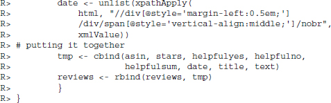
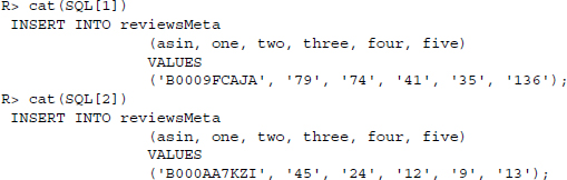
Now that we have gathered all the data we need, it is time to store it in the database. There are two tables in the database that are set up to include the data: reviewsMeta for review data at the level of products and reviews for data at the level of individual reviews. For both tables, we construct SQL INSERT statements for each line of the data frame and loop through them to input the information into the database. The SQL statements for inserting data into the reviewsMeta table should have the following abstract form:

To achieve this, we use two calls to str_c(). The inner call combines the values to be stored in a string, where each value is separated by ’, ’. These strings are then enclosed by the rest of the statement INSERT INTO ... (’ and ’); to complete the statement.
The first two entries in the resulting vector of statements look as follows
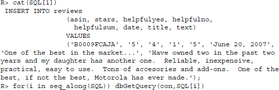
Now we can loop through the vector and send each statement via dbGetQuery() to the database.
R> for(i in seq_along(SQL)) dbGetQuery(con, SQL[i])
The process for storing the data of the individual reviews is similar to the one presented for reviewsMeta. First, we combine values and SQL statement snippets to form a vector of statements, and then we loop through them and use dbGetQuery() to send them to the database.
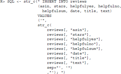
Again, consider the first entry in the resulting vector of statements.
17.3 Analyzing the data
Now that we have the reviews in a common database, we can go on to perform the sentiment scoring of the texts. After some data preparation in the next section, we make a first try by scoring the texts based on a sentiment dictionary. We go on to estimate the sentiment of the reviews using the structured information to assess whether we are able to train a classifier that recovers the sentiment of the texts that are not in the training corpus.
Let us begin by setting up a connection to the database and listing all the available tables in the database.
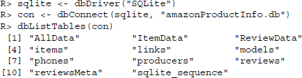
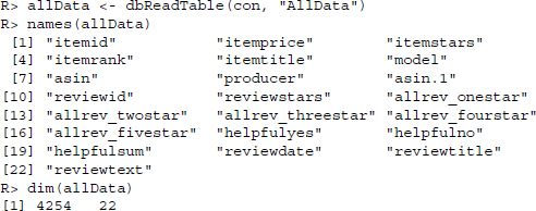
We read the AllData table to a data.frame and output the column names and the dimensions of the dataset. AllData is a view—a virtual table—combining information from several tables into one.
17.3.1 Data preparation
For data preparation, we rely on the tm package that was already introduced in Chapter 10. We also apply the textcat package to classify the language of the text and the RTextTools package to perform the text mining operations further below. vioplot provides a plotting function that is used in the next section.
R> library(tm)
R> library(textcat)
R> library(RTextTools)
R> library(vioplot)
Before setting up the text corpus, we try to discard reviews that were not written in English. We do this by using the textcat package which categorizes the language of a text by considering the sequence of letters. Each language has a particular pattern of letter sequences. We can make use of this information by counting the sequences—so-called n-grams—in a text and comparing the empirical patterns to reference texts of known language.1 The classification method is fairly accurate but some misclassifications are bound to happen. Due to the data abundance, we discard all texts that are estimated to not be written in English. We also discard reviews where the review text is missing.
R> allData$language <- textcat(allData$reviewtext)
R> dim(allData)
R> allData <- allData[allData$language == ”english”,]
R> allData <- allData[!is.na(allData$reviewtext),]
R> dim(allData)
[1] 3748 23
Next, we set up a corpus of all the textual reviews.
R> reviews <- Corpus(VectorSource(allData$reviewtext))
We also perform the preparation steps that were introduced in Chapter 10, that is, we remove numbers, punctuation, and stop words; convert the texts to lower case; and stem the terms.
R> reviews <- tm_map(reviews, removeNumbers)
R> reviews <- tm_map(reviews, str_replace_all, pattern = ”[[:punct:]]”, replacement = ” ”)
R> reviews <- tm_map(reviews, removeWords, words = stopwords(”en”))
R> reviews <- tm_map(reviews, tolower)
R> reviews <- tm_map(reviews, stemDocument, language = ”english”)
R> reviews
A corpus with 3748 text documents
17.3.2 Dictionary-based sentiment analysis
The simplest way to score the sentiment of a text is to count the positively and negatively charged terms in a document. Researchers have proposed numerous collections of terms expressing sentiment. In this application, we use the dictionary that is provided by Hu and Liu (2004) and Liu et al. (2005).2 It consists of two lists of several thousand terms that reveal the sentiment orientation of a text. We load the lists and discard the irrelevant introductory lines.
R> pos <- readLines(”opinion-lexicon-English/positive-words.txt”)
R> pos <- pos[!str_detect(pos, ”⁁;”)]
R> pos <- pos[2:length(pos)]
R> neg <- readLines(”opinion-lexicon-English/negative-words.txt”)
R> neg <- neg[!str_detect(neg, ”⁁;”)]
R> neg <- neg[2:length(neg)]
We stem the lists using the stemDocument() function and discard duplicates.
R> pos <- stemDocument(pos, language = ”english”)
R> pos <- pos[!duplicated(pos)]
R> neg <- stemDocument(neg, language = ”english”)
R> neg <- neg[!duplicated(neg)]
Let us have a brief look at a sample of positive and negative terms to check whether the dictionary contains plausible entries.
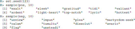
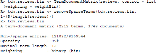
The randomly drawn words seem to plausibly reflect positive and negative sentiment—although we hope that no reviewed phone is reviewed as suitable for martyrdom seekers. We go on to create a term-document matrix where the terms are listed in rows and the texts are listed in columns. In an ordinary term-document matrix, the frequency of the terms in the texts would be displayed in the cells. Instead, we count each term only once, regardless of the frequency with which it appears in the text. We thus argue that the simple presence or absence of the terms in the texts is a more robust summary indicator of the sentiment orientation of the texts. This is done by adding the control option weighting of the function TermDocumentMatrix() to weightBin. We also discard terms that appear in five reviews or less.
To calculate the sentiment of the text, we shorten the matrices to contain only those terms with a known orientation—separated by positive and negative terms. We sum up the entries for each text to get a vector of frequencies of positive and negative terms in the texts. To summarize the overall sentiment of the text, we calculate the difference between positive and negative terms and discard differences of zero, that is, reviews that do not contain any charged terms or where the positive and negative terms cancel each other out.
R> pos.mat <- tdm.reviews.bin[rownames(tdm.reviews.bin) %in% pos, ]
R> neg.mat <- tdm.reviews.bin[rownames(tdm.reviews.bin) %in% neg, ]
R> pos.out <- apply(pos.mat, 2, sum)
R> neg.out <- apply(neg.mat, 2, sum)
R> senti.diff <- pos.out - neg.out
R> senti.diff[senti.diff == 0] <- NA
Let us inspect the results of the sentiment coding. First, we call some basic distributional properties.
![]()
The mean review is positive (4.36 positive words on average), but the extremes are considerable, especially concerning the upper end of the distribution. The most positive text contains a net of 51 positive terms.3 What this summary indicates is the obstacle of extreme variation in the length of the reviews.
R> range(nchar(allData$reviewtext))
[1] 76 23995
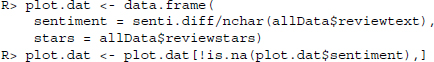
While the shortest review contains no more than 76 characters, the largest stemmed (!) review encompasses no fewer than 23,995. Students occasionally submit shorter term papers. Since we consider the differences between positive and negative reviews this should not be a dramatic problem. Nevertheless, we divide the sentiment difference by the number of characters in the review to get the estimates on a common metric. First, we set up a data frame with data that we want to plot and discard observations where the estimated sentiment is 0.
Using the vioplot() function from the vioplot package, we create a violin plot, a box plot-kernel density plot hybrid (Adler 2005; Hintze and Nelson 1998).
R> vioplot(
R> plot.dat$sentiment[plot.dat$stars == 1],
R> plot.dat$sentiment[plot.dat$stars == 2],
R> plot.dat$sentiment[plot.dat$stars == 3],
R> plot.dat$sentiment[plot.dat$stars == 4],
R> plot.dat$sentiment[plot.dat$stars == 5],
R> horizontal = T,
R> col = ”grey”)
R> axis(2, at = 3, labels = ”Stars in review”, line = 1, tick = FALSE)
R> axis(1, at = 0.01, labels = ”Estimated sentiment by number of characters”, line = 1, tick = FALSE)
The result is plotted in Figure 17.1. We find that the order of estimated sentiment is in line with the structured reviews. The more stars a reviewer has given a product, the better the sentiment that is expressed in the textual review and vice versa. However, there is also a considerable overlap of the five categories and even for one-star ratings we have an overall mean positive sentiment. Apparently, our estimates only roughly capture the expressed sentiment.
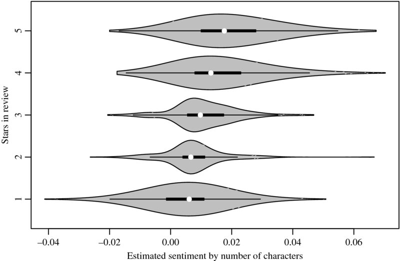
Figure 17.1 Violin plots of estimated sentiment versus product rating in Amazon reviews
One alternative to estimating the sentiment of the review text is to consider the sentiment that is expressed in the headline. The advantage of this is that the headline often contains a summary statement of the review and is thus more easily accessible to a sentiment estimation. We create a corpus of the review titles and perform the same data preparation as before.
R> # Set up the corpus of titles
R> titles <- Corpus(VectorSource(allData$reviewtitle))
R> titles
R> # Perform data preparation
R> titles <- tm_map(titles, removeNumbers)
R> titles <- tm_map(titles, str_replace_all, pattern = ”[[:punct:]]”, replacement = ” ”)
R> titles <- tm_map(titles, removeWords, words = stopwords(”en”))
R> titles <- tm_map(titles, tolower)
R> titles <- tm_map(titles, stemDocument, language = ”english”)
R> # Set up term-document matrix
R> tdm.titles <- TermDocumentMatrix(titles)
R> tdm.titles <- removeSparseTerms(tdm.titles, 1-(5/length(titles)))
R> tdm.titles
R> # Calculate the sentiment
R> pos.mat.tit <- tdm.titles[rownames(tdm.titles) %in% pos, ]
R> neg.mat.tit <- tdm.titles[rownames(tdm.titles) %in% neg, ]
R> pos.out.tit <- apply(pos.mat.tit, 2, sum)
R> neg.out.tit <- apply(neg.mat.tit, 2, sum)
R> senti.diff.tit <- pos.out.tit - neg.out.tit
R> senti.diff.tit[senti.diff.tit == 0] <- NA
Since the sentiment difference has fewer than 10 distinct values in this case, we plot the estimates as points rather than as density distributions. For the same reason, we do not divide our results by the number of characters in the titles, as they are all of roughly the same length. A random jitter is added to the points before plotting. As there are only five categories in the structured reviews, we can better inspect our results visually if we add some noise to the points.
Again, we observe a rough overlap between the number of stars that were assigned by the reviewers and the estimated sentiment in the title (see Figure 17.2). Nevertheless, our estimates are frequently somewhat off the mark. We therefore move on to an alternative text mining technique in the next section.
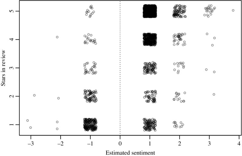
Figure 17.2 Estimated sentiment in Amazon review titles versus product rating. The data are jittered on both axes.
17.3.3 Mining the content of reviews
Chapter 10 discussed the possibilities of applying text mining to estimate the topical categories of text. This is done by assigning labels to a portion of a text corpus and estimating the labels for the unlabeled texts based on similarities in the word usages. There is no technical constraint on the type of label that we can try to estimate. This is to say that we do not necessarily have to estimate the topical emphasis of a text. We might as well estimate the sentiment that is expressed in a text as long as we have a labeled training set.
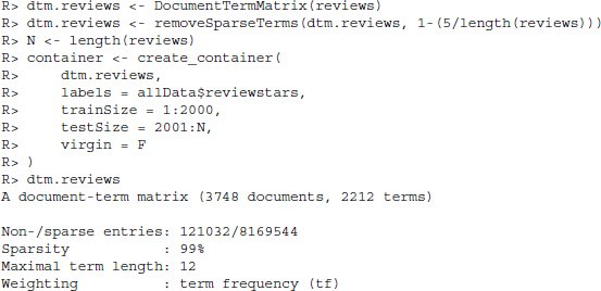
We set up a document-term matrix that is required by the RTextTools package. We remove the sparse terms and set up the container for the estimation. The first 2000 reviews are assigned to the training set and the remaining batch of roughly 2000 we use for testing the accuracy of the models.
We train the maximum entropy and support vector models and classify the test set of reviews.
R> maxent.model <- train_model(container, ”MAXENT”)
R> svm.model <- train_model(container, ”SVM”)
R> maxent.out <- classify_model(container, maxent.model)
R> svm.out <- classify_model(container, svm.model)
Finally, we create a data frame of the results, along with the correct labels.
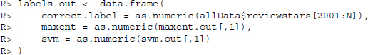
As before, we plot the results as a point cloud and add a random jitter to the points for visibility.
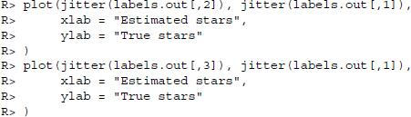
The results are displayed in Figures 17.3 and 17.4—the data are jittered on both axes. Using either classifier we find that both procedures result in fairly accurate predictions of the number of stars in the review based on the textual review.
Figure 17.3 Maximum entropy classification results of Amazon reviews
Figure 17.4 Support vector machine classification results of Amazon reviews
There are more classifiers implemented in the RTextTools package. Go ahead and try to estimate other models on the dataset. You simply have to adapt the algorithm parameter in the train_model() function.4 You might also like to generate the modal estimate from multiple classifiers in order to further improve the accuracy of the sentiment classification of the textual reviews.
17.4 Conclusion
In this chapter, we have applied two techniques for scoring the sentiment that is expressed in texts. On the one hand, we have estimated the sentiment of product reviews based on the terms that are used in the reviews. On the other, we have shown that supervised text classification is not necessarily restricted to the topical category of texts. We can classify various aspects in texts, as long as there is a labeled training set.
The scoring of the texts is simplified in this instance, as product reviews refer to precisely one object—the product. This is to say that negative terms anywhere in the texts will most likely refer to the product that is being reviewed. Compare this to a journalistic text where multiple objects might be discussed in a way that it is not straightforward to estimate the object that a negative term refers to. Consequently, we cannot as easily make the implicit assumption of the analyses in this chapter that a term anywhere in the text refers to one particular object. Moreover, the sentiment in a product review is also simple to score as it is written to explicitly express a sentiment. Again, compare this to a journalistic text. While the text might in fact express a sentiment toward a topic or toward particular actors, the sentiment is ordinarily expressed in more subtle ways.