
Chapter 2
Survey
The Autodesk® AutoCAD® Civil 3D® software supports a collaborative workflow in many aspects of the design process but especially in the survey realm. Accurate data starts outdoors. A survey that has been consistently and correctly coded in the field can save hours of drafting time. Surveyors can collect line information for such things as swales, curbs, or even pavement markings and communicate this digitally to data collectors.
Civil 3D can often eliminate the need for third-party survey software because it can download and process survey data directly from a data collector. To enter data in a manner that is easily digested by Civil 3D, your survey process should incorporate the information from this chapter.
In this chapter, you will learn to:
- Properly collect field data and import it into Civil 3D.
- Set up description key and figure databases.
- Translate surveys from assumed coordinates to known coordinates.
- Perform traverse analysis.
Setting Up the Databases
![]()
Before any project-specific data is imported, you should do a bit of initial setup to improve the translation between the field and the office. For this chapter you will need to see your Survey tab in Toolspace. If you do not see this tab, click the Survey button on the Home tab ![]() Palettes panel.
Palettes panel.
![]()
Your survey database defaults, equipment database, linework code set, and the figure prefix database should be in place before you import your first survey. You can find the location of these files by going to Toolspace ![]() Survey tab and clicking the Survey User Settings button in the upper-left corner of the palette. The dialog shown in Figure 2.1 opens.
Survey tab and clicking the Survey User Settings button in the upper-left corner of the palette. The dialog shown in Figure 2.1 opens.

Figure 2.1 Survey User Settings dialog
The survey database settings path points to the locations of the equipment database, figure prefix database, and linework code sets. Note that these files are separate from the Civil 3D template. These databases are separate files that reside in C:ProgramDataAutodeskC3D 2016enuSurvey by default. It is common practice to place these files on a network server so your organization can share them. You can set these paths while installing the software. Otherwise, change the paths in the Survey User Settings dialog on each individual computer, and they will “stick” regardless of which drawing you have open.
Survey Database Defaults
Every survey database that is created for a project has settings that you will need to examine and verify. To create a new survey database for a project, click the Import Survey Data button from the Home tab of the ribbon or right-click Survey Databases from Toolspace ![]() Survey tab and select New Local Survey Database.
Survey tab and select New Local Survey Database.
Once the new database is created, you will be able to edit its properties, as outlined in the upcoming exercise. The Survey Database Settings dialog contains these settings:
- Units Most likely, the Units setting is the only one you will ever need to modify in the Survey Database Settings dialog. Pay close attention to the units (Imperial vs. US Foot) if you choose not to select a master coordinate zone. This section is where you set your master coordinate zone for the database.
- Potentially, your drawing and your incoming survey data may have different coordinate systems. If you insert any information stored in the database into a drawing with a different coordinate zone, the program will automatically translate that data to the drawing coordinate zone (upon initial import only). Your coordinate zone units will lock in the distance units in the Units section. Although usually not necessary, you can also set the angle, direction, temperature, and pressure specific to the survey database here.
- PrecisionThis section is where you define and store the precision information of angles, distance, elevation, coordinates, and latitude and longitude specific to the database. Note that this affects display precision for the survey interface and is independent from label precision and drawing precision set in the Drawing Settings dialog discussed in Chapter 1, “The Basics.”
- Measurement Type Defaults This section lets you tell Civil 3D what type of information to expect when importing survey data from a file. The information can be measurement types, such as angle type, distance type, vertical type, and target type.
- Measurement Corrections This section is used to define the methods (if any) for correcting measurements. You will probably not need to change anything in this section because most data collectors will have processed this for you.
- Traverse Analysis Defaults This section is where you choose what types of traverse analysis you want to perform. You can control the method you want to use and required precision and tolerances for each. There are four types of 2D traverse analysis methods: Compass Rule, Transit Rule, Crandall Rule, and Least Squares Analysis.
- There are three potential types of 3D traverse analyses: Length Weighted Distribution, Equal Distribution, and Least Squares Vertical. Vertical options for Least Squares will be available only if it is first set as the Horizontal Adjustment Method. Of course, you can always choose None to omit that calculation from the analysis.
- Least Squares Analysis Defaults If you are performing a Least Squares analysis, you must specify 2-Dimensional or 3-Dimensional adjustment type. Use 3-Dimensional if you are performing both horizontal and vertical Least Squares adjustment.
- Survey Command Window In the rare event that you'll need it, the Survey Command window is the interface for manual survey tasks and for running survey batch files. This section lets you define the default settings for this window.
- Error Tolerance Set tolerances for the survey database in this section. If you perform an observation more than one time and the tolerances established here are not met, an error will appear in the Survey Command window, and you will be asked what action you want to take.
- Extended Properties You may work with LandXML files that contain information beyond traditional “P,N,E,Z,D” data. If this is the case, you will want to turn both Extended Properties options to Yes. Create New Definitions Automatically will add extended properties to your survey database and populate the fields from the imported file. Display Warnings For Missing Required Fields will display the Panorama interface if there is missing information in the imported file.
- Change Reporting It is a great idea to turn this option to Yes by setting Logging Enabled to Yes. This will create an audit trail of changes to the database that occur after import. The changes to the database are stored in a LOG file (
*.log) located in the same directory as your survey database. At any time, you can access the contents of the log by right-clicking the name of the survey database and selecting Display Change Report.
When you first configure your survey database settings, it is a good idea to create a test database for setting the defaults. Because survey database settings are independent of which drawing you are in, you can perform these steps with any file open. To create the test database, follow these steps:
- In the Toolspace
 Survey tab, right-click Survey Databases.
 - Select Set Working Folder.
Civil 3D will create a working folder to contain your survey database. Ideally, this will be stored in a network location for your organization's projects. For examples in this book, this will be set to your local C drive.
- Verify that the
C:Civil 3D Projectsfolder is highlighted and click OK. - In the Toolspace Survey tab, right-click Survey Databases and choose New Local Survey Database.
- Name the new database Test and click OK to continue.
- Right-click the new Test database and select Edit Survey Database Settings.
- Set your desired defaults for units, precision, and other options, as shown in Figure 2.2.

Figure 2.2 Survey Database Settings dialog
- Click the Export Settings To A File button.

- Save the settings to the folder specified in the Survey User Settings dialog (shown earlier in Figure 2.1) as
MySettings.sdb_setand then click Save and then OK.
To delete your Test database, you will need to close the database from the Survey tab. To do so, locate the database in Toolspace ![]() Survey tab. Right-click it and select Close Survey Database. Using Windows Explorer, you can then browse to the working folder containing the database and delete it. There is no way to delete a survey database from within the software.
Survey tab. Right-click it and select Close Survey Database. Using Windows Explorer, you can then browse to the working folder containing the database and delete it. There is no way to delete a survey database from within the software.
The Equipment Database
![]()
The equipment database is where you set up the various types of survey equipment that you are using in the field. Doing so allows you to apply the proper correction factors to your traverse analyses when it is time to balance your traverse. Civil 3D comes with a sample piece of equipment for you to inspect to see what information you will need when it comes time to create your equipment. The Equipment Database Manager dialog provides all the default settings for the sample equipment in the equipment database. On the Survey tab of Toolspace, expand Equipment Databases, right-click Sample, and click Manage Equipment Database to access this dialog, shown in Figure 2.3.

Figure 2.3 Use Equipment Database Manager.
Figure 2.3 shows the settings for a specific model of total station—the Trimble S8. When you input this data to an equipment database, consult your instrument's datasheet for specifications. The specifics of total station equipment will vary by manufacturer and model.
You will want to create your own equipment entries and enter the specifications for your particular total station. Add a new piece of equipment to the database by clicking the plus sign at the top of the Equipment Database Manager window. If you are unsure of the settings to enter, refer to the user documentation that you received when you purchased your total station. Also be careful that you aren't applying a correction that hasn't already been applied in the gun itself such as prism offset.
The Figure Prefix Database
![]()
![]()
The figure prefix database is used to translate descriptions in the field to lines in CAD. These survey-generated lines are called figures. If a description matches a listing in the figure prefix database, the figure is assigned the properties and style dictated by the database (see Figure 2.4).

Figure 2.4 The Figure Prefix Database Manager
The Figure Prefix Database Manager contains these columns:
- Name The figure name is important because it must match the description used by the surveyor in the imported survey file. For example, if the surveyor collects points along the back of curb using the description BC, then there must be a figure name called BC in the figure prefix database in order to create linework or figures with those points using the properties specified in the database. If the figure name doesn't match up with a figure prefix, the linework will be drawn using default settings specified on the Settings tab.
- Breakline Placing a check mark in this column will allow you to flag a figure as a breakline. The most powerful use of this setting is the Create Breaklines command on the context menu of the Figures collection located within the survey database on the Toolspace Survey tab. Figures with this setting on can be added to the definition of a surface model. Even if you don't flag a figure as a breakline, you can still add it to a surface model manually.
- Lot Line This column specifies whether the figure should behave as a parcel segment. If a closed area is formed with figures of this kind, a parcel is formed automatically.
- Layer This column specifies the insertion layer of the figure. If the layer already exists in the drawing, the figure will be placed on that layer. If the layer does not exist in the drawing, the layer will be created and the figure placed on the newly created layer. In the case of the latter, you may need to manually reset the layer properties so your figures display according to your standards. In the case where an incoming figure name doesn't match up with a figure prefix, the newly created figure will be placed on the layer specified for Survey Figure on the Object Layer tab of Drawing Settings. Drawing Settings were discussed in Chapter 1.
- StyleThis column specifies the style to be used for each figure. Figure styles will override color and linetype of the insertion layer if the style layer is set to something other than Layer 0. See the section on linear object styles in Chapter 19, “Object Styles,” for more information on this type of style.
- Site This column specifies which site the figures should reside on when inserted into the drawing. As with previous settings, if the site exists in the drawing, the figure will be inserted into that site. If the site does not exist in the drawing, a site will be created with that name, and the figure will be inserted into the newly created site.
Remember that figure prefix databases are not drawing specific. The only reason a drawing is needed is to access the styles that the figures will use.
You'll explore these settings in a practical exercise:
- Open the drawing
0201_SurveySetup.dwgor0201_SurveySetup_METRIC.dwg, which you can download from this book's web page,www.sybex.com/go/masteringcivil3d2016.This file contains the survey figure styles needed to complete this exercise.
- In Toolspace Survey tab, right-click Figure Prefix Databases and select New.
The New Figure Prefix Database dialog opens.
- Enter Mastering Civil 3D in the Name text box and click OK to dismiss the dialog.
If you expand the Figure Prefix Database listing, you will see the Mastering Civil 3D entry.
- Right-click the newly created Mastering Civil 3D figure prefix database and select Manage Figure Prefix Database.
The Figure Prefix Database Manager will appear.
- Select the white + symbol in the upper-left corner of the Figure Prefix Database Manager to create a new figure prefix.
- Click the default name, Sample, and change the name of the figure prefix to BB (for Bottom of Bank).
- Click the check box next to the word No in the Breakline column. This will turn into a Yes, indicating that it will contain the breakline property.
Leave the box in the Lot Line column unchecked so that the figure will not be treated as a parcel segment.
- In the Layer column, select V-SURV-FIGR.
- In the Style column, select BB.
- In the Site column, leave the name of the site set to Survey Site.
- Complete the figure prefix database with the values shown in Table 2.1.
Table 2.1 Figure settings
Name Breakline Lot Line Layer Style Site BLDG No No V-SURV-FIGR BLDG SURVEY SITE CL Yes No V-SURV-FIGR CL SURVEY SITE DL Yes No V-SURV-FIGR DL SURVEY SITE DW Yes No V-SURV-FIGR DW SURVEY SITE EC Yes No V-SURV-FIGR EC SURVEY SITE EG Yes No V-SURV-FIGR EG SURVEY SITE EP Yes No V-SURV-FIGR EP SURVEY SITE PPE No No V-SURV-FIGR ELEC SURVEY SITE PROP No Yes V-SURV-FIGR PROP SURVEY SITE TB No No V-SURV-FIGR TB SURVEY SITE Hint: For figures with similar properties, select a figure definition already in the database and then use the Copy Figure Prefix button.

- Click OK to dismiss the Figure Prefix Database Manager.
Keep this drawing open to use in the next portion of the exercise.
You can choose whether lines are automatically formed in the linework code set when they match one of these figure prefixes.
The Linework Code Set Database
![]()
The linework code set (Figure 2.5) lists what designators are used to start, stop, continue, or add segments to lines. For example, the B code that is typically used to begin a line can be replaced with an S, RT can be simplified to R for a right turn, and PC and PT can be used to begin and end curves. Linework code sets allow a survey crew to customize their data-collection techniques based on methods used by various types of software not related to Civil 3D.

Figure 2.5 The Edit Linework Code Set dialog
Configuring Description Keys for Point Import
![]()
Description keys bridge the gap between the field and the office. Unlike the linework code set and figure prefix database, which are each external files, description keys should be created and saved in your Civil 3D template. The description key set is a listing of field descriptions and parameters that control how points look and behave once they are imported into or manually created in Civil 3D.
For example, a surveyor collects a point with the description FH to indicate a fire hydrant. When the file is imported into Civil 3D either through the survey database or by point import from a text file (as you will do in Chapter 3, “Points”), it will be checked against the description key set. If FH exists in the list, as it does in Figure 2.6, then the styles, format, layer, and several other parameters are applied to the point as it is placed in the drawing.

Figure 2.6 Description key set
To access your description key set, you will need to expand Toolspace ![]() Settings tab
Settings tab ![]() Point
Point ![]() Description Key Sets.
Description Key Sets.
Right-click the description key set and select Edit Keys; the Description Key Editor will open (using the Panorama interface) with the following columns for you to edit:
- Code The code is the raw description or field code entered by the person collecting or creating the points. The code works as an identifier for matching the point with the correct description key. Click inside this field to activate it and then type your desired code. Wildcards are useful when more information is added to the shot in addition to the field code. Right-click an existing code to copy or create a new description key or delete an existing one.
- Codes are case sensitive! The code
fhis read differently fromFH. A match to the description key set will not be made if the capitalization does not match perfectly. - Style Style refers to the point style that will be applied to points that meet the code criteria. Check the box and then click inside the field to activate a point style selection dialog. By default, styles set here will take precedence over styles set elsewhere (unless overridden in a point group, see Chapter 3). For more information on creating or modifying point styles, see Chapter 19.
- Point Label StyleThis is the point label style that will be applied to points that meet the code criteria. Check the box and then click inside the field to activate a style selection dialog. By default, styles set here will take precedence over styles set elsewhere (unless overridden in a point group). For more information on creating or modifying point label styles, see Chapter 18, “Label Styles.”
- Format The Format column can convert a surveyor's shorthand into something that is more drafter friendly. In Civil 3D terms, the Format column converts the raw description to the full description. The default of
$*means the raw description and full description will have the same value. You can also use$+, which means that information after the main description will appear as the full description. In Figure 2.6, Format will convert all codes starting with MB to a full description of MAILBOX. - If a survey crew is consistent in coding, even fancier formats can be used. The code should always come first, but the crew can use a space to indicate a parameter.
- Consider this example raw description:
TR 30 PINE ELIM.TRis the code, or$0. Parameter 1 is 30, or$1in the Format field.PINEis the second bit of information after the code referred to as parameter 2, or$2.ELIMis the third item after the code, so it is$3. Based on the example description key set in Figure 2.6, this would translate to a full description ofPINE 30. You can have up to nine parameters after the code if your survey crew is feeling verbose. Table 2.2 shows some example formats and the corresponding full description.Table 2.2 Format examples
Raw Description Format Full Description TR 30 PINE ELIM TreeTree TR 30 PINE ELIM $*TR 30 PINE ELIM TR 30 PINE ELIM $0TR TR 30 PINE ELIM $1”30 ”TR 30 PINE ELIM $2PINE TR 30 PINE ELIM $3ELIM TR 30 PINE ELIM $2 $1PINE 30 TR 30 PINE ELIM $+30 PINE ELIM - Layer Points that match a description key will be inserted on the layer specified here. Click inside this field to activate a layer selection dialog. The layer set here will take precedence over layer defaults set in the point command settings or the point creation tools.
- Scale Parameter The Scale parameter is used to tell Civil 3D which bit of information after the code will be used to scale the symbol. By default, it is checked, but it won't do anything unless Apply To X-Y is also selected. Once you enable Apply To X-Y (or Apply To Z, which is less frequently used), you can change which parameter contains scale information.
- In our example, TREE 30 PINE ELIM, 30 (
$1) is the Scale parameter. - Fixed Scale Factor Fixed Scale Factor is an additional scale multiplier that can be applied to the symbol size. A common use of Fixed Scale Factor is to convert a field measurement of inches to feet. If the 30 in our example represents a dripline measurement and is meant to be feet, no Fixed Scale Factor is needed. However, if the 30 represents inches (i.e., a trunk diameter), you would need to turn on Fixed Scale Factor and set the value to 0.0833.
- Use Drawing Scale In most cases, you will leave this option unchecked. By default, marker styles dictate that they will grow or shrink based on the annotative scale of the drawing. Generally, this setting is not needed unless you want to scale your point symbol based on a parameter in addition to the scale factor.
- Apply To X-Y If you want to scale symbols based on information in the field code, you need to turn this option on by placing a check mark in the box. This option works with the marker style and the Scale parameter to increase the size of an item to a scale indicated by the surveyor in the raw description.
- Apply To Z In most cases, you will leave this option unchecked. Most marker symbols are 2D blocks, so selecting this option will have no effect on the point. If your marker symbol consists of a 3D block, it will be stretched by the parameter value, which is rarely needed.
- Marker Rotate Parameter, Marker Fixed Rotation, Label Rotate Parameter, Label Fixed Rotation, and Rotation Direction These options are similar to the scale factor parameter except they dictate the rotation of a symbol or label. They are not widely used, however, because it is often more time effective to have the drafter rotate the points in CAD than to have the surveyor key in a rotation. If you would like to rotate the points for readability, the better method to rotate the text is in the point label style (discussed in Chapter 18).
Creating a Description Key Set
Description key sets appear on the Toolspace ![]() Settings tab, under the Point branch. You can create a new description key set as follows:
Settings tab, under the Point branch. You can create a new description key set as follows:
- Right-click the Description Key Sets collection and choose New, as shown in Figure 2.7.

Figure 2.7 Creating a new description key set on the Settings tab of Toolspace
- In the resulting Description Key Set dialog, give your description key set a meaningful name, such as your company name.
- Click OK.
You'll create the actual description keys in another dialog.
Creating Description Keys
To enter the individual description key codes and parameters, expand Toolspace ![]() Settings tab
Settings tab ![]() Point
Point ![]() Description Key Set. Right-click the description key set, as illustrated in Figure 2.8, and select Edit Keys. The DescKey Editor in the Panorama interface appears.
Description Key Set. Right-click the description key set, as illustrated in Figure 2.8, and select Edit Keys. The DescKey Editor in the Panorama interface appears.

Figure 2.8 Editing a description key set
To enter new codes, right-click a row with an existing key in the DescKey Editor and choose New or Copy from the right-click menu, as shown in Figure 2.9.

Figure 2.9 Creating or copying a description key
In the following exercise, you'll create and populate a description key set.
- Continue working in your
0201_SurveySetup.dwgor0201_SurveySetup_METRIC.dwgfile. You must have completed the previous exercise. - From the Toolspace Settings tab, expand the Points branch, right-click Description Key Sets, and click New.
- In the Description Key Set – New DescKey Set dialog, type Mastering Civil 3D in the Name field. Click OK to continue.
- From the Toolspace Settings tab under the Points branch, expand Description Key Sets, right-click the Mastering Civil 3D description key set, and click Edit Keys.
The DescKey Editor will open in Panorama.
- Create the description keys in Table 2.3 by right-clicking a description key line in the list and clicking New or Copy.
Table 2.3 New description keys
Code Style Point Label Style Format Layer BB*Elevation Marker Elevation Only $* V-NODE-TOPO BLDG*Linework No Display $* V-NODE-BLDG CL*Elevation Marker Elevation Only $* V-NODE-TOPO DL*Elevation Marker Elevation Only $* V-NODE-TOPO DW*Elevation Marker Elevation Only $* V-NODE-DRIV EC*Elevation Marker Elevation Only $* V-NODE-CONC EG*Elevation Marker Elevation Only $* V-NODE-GRVL EP*Elevation Marker Elevation Only $* V-NODE-PVMT FH*Hydrant (existing) No Display $* V-NODE-WATR GS*Elevation Marker Elevation Only $* V-NODE-TOPO GUY*Guy Wire No Display $* V-NODE-POWR IPF*Iron Pin Description Only IRON PIN (F) V-NODE-PROP IRF*Iron Pin Description Only IRON ROD (F) V-NODE-PROP MB*Mailbox Description Only MAILBOX V-NODE-SITE PED*Telephone Pedestal Description Only T PED V-NODE-COMM PP*Power Pole No Display $* V-NODE-POWR PROP*Linework No Display $* V-NODE-PROP TB*Elevation Marker Elevation Only $* V-NODE-TOPO TREE*Tree Description Only $1“ $2 V-NODE-TREE TRANS*Transformer Description Only TRANS V-NODE-POWR WM*Water Meter Description Only $* V-NODE-WATR WV*Water Valve Description Only $* V-NODE-WATR You may have noticed an extra description key on the list called New DescKey, which was created by default when the description key set was made. This description key can be deleted by clicking it and selecting Delete from the context menu. Another option would be to edit the entry to represent a description key you need.
When this exercise is complete, you may close the drawing. A saved copy of this drawing (0201_SurveySetup_FINISHED.dwg or 0201_SurveySetup_METRIC_FINISHED.dwg) is available from the book's web page.
Activating a Description Key Set
Once you've created a description key set, you should verify the settings for your commands so that Civil 3D knows to match your newly created points with the appropriate key.
In Toolspace ![]() Settings tab, expand Point
Settings tab, expand Point ![]() Commands and right-click CreatePoints. Select Edit Command Settings, as shown in Figure 2.10.
Commands and right-click CreatePoints. Select Edit Command Settings, as shown in Figure 2.10.

Figure 2.10 Right-click CreatePoints and choose Edit Command Settings.
In the Edit Command Settings – CreatePoints dialog, expand the Points Creation category and ensure that Match On Description Parameters is set to True and that Disable Description Keys is set to False, as shown in Figure 2.11.

Figure 2.11 Verify that Match On Description Parameter is set to True, and Disable Description Keys is set to False.
It is common to have multiple description key sets in your template. You can leverage description key sets for multiple clients or external survey firms that you work with. If you have multiple description key sets, they are all active, but if a set has a duplicate key, the first one Civil 3D runs across will take precedence. For example, if one set uses FL for flowline but a second set uses FL for fence line, the second occurrence of the FL key gets ignored.
You can control the search order from the Toolspace ![]() Settings tab
Settings tab ![]() Points branch by right-clicking Description Keys Sets and selecting Properties. Figure 2.12 shows the Description Key Sets Search Order dialog. Choose a description key set in the list and then use the arrows on the right side of the dialog to set the order. The set listed first takes first priority, then the second, and so on. Note that the listing in the Settings tab may not reflect the true listing in the properties.
Points branch by right-clicking Description Keys Sets and selecting Properties. Figure 2.12 shows the Description Key Sets Search Order dialog. Choose a description key set in the list and then use the arrows on the right side of the dialog to set the order. The set listed first takes first priority, then the second, and so on. Note that the listing in the Settings tab may not reflect the true listing in the properties.

Figure 2.12 The Description Key Sets Search Order dialog
Understanding the Survey Database
Now that you know how to get everything set up, you are probably eager to get some real, live data into your drawing.
First set your survey working folder to your desired survey storage location. The Civil 3D survey database is a set of external database files that reside in your survey working folder. By default, this folder is located in C:Civil 3d Projects. This is another item you will want to send to a network location in your own projects.
On the Toolspace ![]() Survey tab, right-click Survey Databases and select Set Working Folder, as shown in Figure 2.13.
Survey tab, right-click Survey Databases and select Set Working Folder, as shown in Figure 2.13.

Figure 2.13 Set the survey working folder.
In the current version of Civil 3D, this is a different, independent setting from the working folder for data shortcuts (as discussed in Chapter 16, “Advanced Workflows”). Most folks want this on a network location, tucked neatly into the survey folder for the project.
![]()
To create a survey database, either you can right-click and select New Local Survey Database from Toolspace ![]() Survey tab as mentioned earlier, or you can select Import Survey Data from the Home tab's Create Ground Data panel.
Survey tab as mentioned earlier, or you can select Import Survey Data from the Home tab's Create Ground Data panel.
The contents of a survey database are organized into the following categories:
- Import Events Import events provide a framework for viewing and editing specific survey data, and they are created each time you import data into a survey database. The default name for the import event is the same as the imported filename. The Import Event collection contains the networks, figures, and survey points that are referenced from a specific import event and provides an easy way to remove, reimport, and reprocess survey data in the current drawing.

- Survey Queries Survey queries allow users to search for specific information within a survey database. You can use a query to locate and group related survey points and figures. For example, you may want all figures representing power lines in a query with survey points representing power poles. If you create a query containing your utilities, you can isolate specific figures and points to insert into another drawing.

- A survey query can be used in conjunction with a surface. When a query containing points and figures is added to a surface model, the figures are automatically added as breaklines. Figure 2.14 shows an example query that might be used for generating surface data.
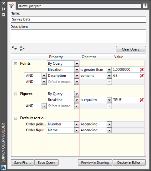
Figure 2.14 Survey database query
- If the survey query you create is worthy of using in other databases, you can export it for use in other databases. Right-click Survey Queries and choose to export or import the query.
- Networks A survey network is a collection of related data that is collected in the field. The network consists of setups, control points, non-control points, directions, and traverses. A survey database can have multiple networks. For example, you can use different networks for different phases of a project.

- Network Groups Network groups are collections of various survey networks within a survey database. These groups can be created to facilitate inserting multiple networks into a drawing at once, simply by dragging and dropping.

- Figures Figures are the linework created by codes and commands entered into the raw data file during data collection. The figure names typically come from the descriptor or description of a point.

- Figure GroupsSimilar to network groups, figure groups are sets of individual figures. These groups can be created to facilitate quick insertion of multiple figures into a drawing.

- Survey Points One of the most basic components of a survey database, points form the basis for each and every survey. Survey points look just like regular Civil 3D point objects, and their visibility can be controlled just as easily. However, one major difference is that a survey point cannot be edited within a drawing. Survey points are locked by the survey database, and the only way of editing them is to edit the observation that collected the data for the points. This provides the surveyor with the confidence that points will not be accidentally erased or edited. Like figures, survey points can be inserted into a drawing either by dragging and dropping from the Toolspace Survey tab or by right-clicking Surveying Points and selecting the Points Insert Into Drawing option.

- Survey Point Groups Just like network groups and figure groups, survey point groups are sets of points that can be easily inserted into a drawing. When these survey point groups are inserted into the drawing, a Civil 3D point group is created with the same name as the survey point group. This point group can be used to control the visibility or display properties of each point in the group.

In the following exercise, you'll create an import event and import an ASCII file with survey data. The survey data includes linework.
- Open the drawing
0202_ImportSurveyData.dwgor0202_ImportSurveyData_METRIC.dwg. If you did not complete the previous exercise, copy the fileMastering Civil 3D.fdb_xdeffrom the dataset toC:ProgramDataAutodeskC3D 2016enuSurvey. Note that this directory is hidden in Windows by default, so you will need to change the folder view options or type this path into the address bar of Windows Explorer. - From the Home tab Create Ground Data panel, click Import Survey Data to open the Import Survey Data Wizard.
- Click Create New Survey Database.
- Enter
Ditch Surveyas the name of the folder in which your new database will be stored. Click OK.Ditch Surveyis now added to the list of survey databases. - With
Ditch Surveyhighlighted, click Edit Survey Database Settings and verify that the Distance units are set to US Foot (or meter). Click OK to dismiss the dialog. - Click Next.
- Set the Data Source Type pull-down to Point File.
- Click the white plus sign on the right side of the Selected Files list to browse to the
0203_ImportPoints.txtor0203_ImportPoints_METRIC.txtfile, which you can download from this book's web page.If necessary, change the File Of Type drop-down selection to Text/Template/Extract File (*.txt).
- Select the file and then click Open, and the name will be listed in the dialog, as shown in Figure 2.15.

Figure 2.15 Select the correct source type, file, and format in the Import Survey Data Wizard.
- Under Specify Point File Format, scroll through the list until you find PENZD (Comma Delimited).
- Highlight the PENZD (Comma Delimited) format.
The preview will show that the correct data type is selected, as shown at the bottom of Figure 2.15.
- Click Next to continue.
- Click Create New Network.
Note that if you forget to create a network to place your points, you will not be able to manipulate this group apart from other points.
- Enter Ditch Survey 4-22-2015 as the name of the network and click OK.
- Highlight the new network and click Next to continue.
- Enter the following settings:
- Set Current Figure Prefix Database to Mastering Civil 3D.
- Set the Process Linework During Import option to Yes.
Be sure Insert Survey Points is set to Yes.
- When your import options match what is shown in Figure 2.16, click Finish.

Figure 2.16 The Import Options page in the Import Survey Data Wizard
- Save the file as
0203_DitchSurvey.dwgto the same location as the rest of your downloaded example files. You will need it in the next exercise.
The data is imported and the linework is drawn; however, there are some mistakes in the coding, which is producing erroneous linework. The following steps will resolve this issue:
- Continue working in the drawing from the previous exercise. In the Toolspace Survey tab, expand Survey Databases and then select Ditch Survey Networks Ditch Survey 4-22-2015 Non-Control Points.
- Right-click Non-Control Points and select Edit to bring up the Non-Control Points Editor in Panorama.
- Scroll to point Number 1104, right-click, and click Zoom To.
The red line represents the flowline of the ditch. Notice in the drawing how the linework crosses over the brown top of bank line to the flowline of another ditch. The points along the ditches were collected simultaneously using the code
DLfor the left side andDL2for the right side. Point 1104 representing the right side was obviously miscoded, and correcting the description in the editor will allow you to reimport the corrected linework. - In Panorama, double-click the Description field.
- Use the arrow keys on your keyboard to move your cursor to the end of the description
DL. - Add
2↲ to the end of the description, as shown in Figure 2.17.
Figure 2.17 Editing the import event to fix the linework representing the ditch flowline
This will be corrected after reprocessing the linework.
The surveyor was simultaneously picking up points for two ditch lines coded
DLandDL2. Miskeying codes is a common mistake when so much data is being collected. - Click the Save icon in the upper-right corner of Panorama and then click the green check mark in the upper right of the palette to apply changes and save your edits.

At this point you should see a yellow exclamation mark symbol next to the network name. This indicates that a change has been made to the survey database that has not yet been processed in the drawing. In the next steps, you will update the network to reflect the change graphically.
- Click Yes if you are asked to apply your changes.
- Right-click the network name (Ditch Survey 4-22-2015) and select Update Network.
- Click Close to dismiss the Survey Network Updated dialog.
Updating the survey network has triggered a change in the figures as indicated by the exclamation mark symbol next to the Figures branch.
- Right-click the Figures collection and select Update Figures.
- Click the green check mark in the upper right of Panorama to dismiss the Event Viewer.
- While still working in Survey Databases Ditch Survey, expand Import Events and select
0203_ImportPoints.txt(0202_ImportPoints_METRIC.txt). - Right-click the import event and select Process Linework to bring up the Process Linework dialog.
- Click OK to reprocess the linework with your updated point description.
The ditch (
DL2) figure line and your drawing should look something like Figure 2.18. Repeat steps 2–3 to zoom to the point again.
Figure 2.18 After editing and reprocessing the linework
- Repeat steps 2–15 for the points in Table 2.4.
Table 2.4 Corrections to non-control points
Number New Description 1134 DL2 1864 DL1 1925 DL 2217 BB1 B 3966 BB1 B 4058 BB2 B 4060 BB1 B For three of the points, you will be adding a Begin command (
B) after the description separated by a space.
When this exercise is complete, you can close the drawing. A saved copy of this drawing (0203_DitchSurvey_FINISHED.dwg or 0203_DitchSurvey_METRIC_FINISHED.dwg) is available from the book's web page.
When you make modifications to survey data, only the Civil 3D database is changed. The original import file remains untouched. The survey database doesn't use the file unless you reimport the data.
If you edit raw data in the Survey tab, Civil 3D will recalculate all affected information. For example, if you modify an instrument height, all elevations that need to be updated will automatically adjust.
Keep in mind that if you edit the source file and reimport, the data in the Civil 3D database (and any edits you made) will be overwritten.
Working with Survey Networks
Once you import survey data into a network, expand the branch to see how Civil 3D helps you make sense of it. In each network, data is organized by type, as shown in Figure 2.19.

Figure 2.19 A typical survey database network with data
- Control Points Control points are created when data from an FBK file is imported. Inside the FBK, control points are prefaced by NE, NEZ, or LAT LONG. You can force any point to be listed as a control point by right-clicking this collection and selecting New.

- Non-Control PointsKeyed-in points, GPS-collected points, and any point brought in through an ASCII file will appear as non-control points. This is the default type if no other information is known about the point.

- Directions The direction from one point to another must be manually entered into the data collector for the direction to show up later in the survey network for editing. The direction can be as simple as a compass shot between two initial traverse points that serves as a rough basis of bearings for a survey job.

- Setups If you imported data that contains setups and observations, Setups is where the meat of the data is found. Every setup, as well as the points (side shots) located from that setup, can be found listed here. Setups will contain two components: the station (or occupied point) and the backsight. To see or edit the observations located from the setup, right-click Setups and select Edit Setups That Observe. Figure 2.20 shows the interface for editing setups. Backsight orientation and instrument heights can also be changed in this dialog.


Figure 2.20 Setups can be changed in the Setups Editor
- Traverses The Traverses section is where new traverses are created or existing ones are edited. These traverses can come from your data collector, or they can be manually entered from field notes via the Traverse Editor, as shown in Figure 2.21. You can view or edit each setup in the Traverse Editor, as well as the traverse stations located from that setup.


Figure 2.21 The Traverse Editor
- Once you have defined a traverse, you can adjust it by right-clicking its name and selecting Traverse Analysis. You can adjust the traverse either horizontally or vertically, using a variety of methods. The traverse analysis can be written to text files to be stored, and the entire network can be adjusted on the basis of the new values of the traverse.
In the following exercise, you will adjust a traverse:
- Create a new drawing from the
_AutoCAD Civil 3D (Imperial) NCS.dwt(_AutoCAD Civil 3D (Metric) NCS.dwt) template file. - Navigate to the Toolspace Survey tab.
- Right-click Survey Databases and select New Local Survey Database.
The New Local Survey Database dialog opens.
- Enter
Traverseas the name of the folder in which your new database will be stored. - Click OK to dismiss the dialog.
The Traverse survey database is created as a branch under the Survey Databases branch.
- Expand the Traverse branch, right-click Networks, and select New.
The New Network dialog opens.
- Expand the Network branch in the dialog if needed.
- Name your new network Traverse Practice and click OK.
- Right-click the Traverse Practice network and select Import Import Field Book.
- Select the file
0204_Traverse.fbk(0204_Traverse_METRIC.fbk), which you can download from this book's web page, and click Open.The Import Field Book dialog opens.
- Make sure you have checked the boxes shown in Figure 2.22.

Figure 2.22 The Import Field Book dialog
There is no linework in this file because it is just traverse shots.
- Click OK. Double-click your middle mouse wheel to zoom extents to get a look at the imported traverse.
The Traverse Practice network is now listed as a branch under Toolspace
Prospector Survey Networks. - Save the drawing as
0204_Traverse.dwgfor the next exercise.
Looking back at the Toolspace ![]() Survey tab, expand the network you created earlier and inspect the data. You have one control point in the northwest corner that was manually entered into the data collector. There is one direction, and there are four setups. Each setup combines to form a closed polygonal shape that defines the traverse. Notice that there is no traverse definition. In the following exercise, you'll create that traverse definition for analysis.
Survey tab, expand the network you created earlier and inspect the data. You have one control point in the northwest corner that was manually entered into the data collector. There is one direction, and there are four setups. Each setup combines to form a closed polygonal shape that defines the traverse. Notice that there is no traverse definition. In the following exercise, you'll create that traverse definition for analysis.
Continue working in the drawing from the previous exercise:
- Go to Toolspace Survey Survey Databases Traverse Networks Traverse Practice; then right-click Traverses and select New to open the New Traverse dialog.
- Name the new traverse Traverse 1.
- Type 2 as the Initial Station point number and press Enter.
The traverse will now pick up the rest of the stations in the traverse and enter them in the next box.
- Verify that the points on the traverse match what is shown in Figure 2.23.

Figure 2.23 Defining a new traverse
- Click OK.
- Right-click Traverse 1 in the Item View of Toolspace. Select Traverse Analysis.
- In the Traverse Analysis dialog, ensure that Yes is selected for Do Traverse Analysis and Do Angle Balance.
- Select Least Squares for both Horizontal Adjustment Method and Vertical Adjustment Method.
- Set both Horizontal Closure Limit 1:X and Vertical Closure Limit 1:X to 20,000.
- Leave Angle Error Per Set at the default.
- Make sure the option Update Survey Database is set to Yes.
The Traverse Analysis dialog will look like Figure 2.24.

Figure 2.24 Specify the adjustment method and closure limits in the Traverse Analysis dialog.
- Click OK.
The analysis is performed, and four text files are opened that show the results of the adjustment. These files are automatically saved in the survey working folder under the same directory as the survey database (in this example, it should be C:Civil 3D ProjectsTraverseTraverse 1).
Note that if you look back at your survey network, all points are now control points because the analysis has upgraded all the points to control point status. Also, error ellipses are displayed in the drawing area at each station adjusted. The size of error ellipses are controlled by a scale factor set in the Survey Network style. If you are seeing extra-large ellipses, it is not an indication of an extra-large error. Styles will be discussed more in depth in Chapter 19.
Figure 2.25 shows the Traverse 1 Raw Closure.trv and Traverse 1 Vertical Adjustment.trv files that are generated from the analysis. The raw closure file shows that your new precision is well within the tolerances set in step 8. The vertical adjustment file describes how the elevations have been affected by the procedure.

Figure 2.25 Horizontal and vertical traverse analysis results
Traverse 1.lso is the output file displaying the adjustments of the traverse analysis. The first part of the file, shown in Figure 2.26, displays the various observations along with their initial measurements, standard deviations, adjusted values, and residuals. You can view other statistical data at the beginning of the file.

Figure 2.26 Statistical and observation data portion of text file
Figure 2.27 shows the second portion of this text file (you will need to scroll down to see it) and displays the adjusted coordinates, the standard deviation of the adjusted coordinates, and information related to error ellipses displayed in the drawing. If the deviations are too high for your acceptable tolerances, first check the instrument settings and tolerances in the equipment database. If everything is set correctly, you may need to redo the work or edit the field book.

Figure 2.27 Adjusted coordinate information portion of text file
Figure 2.28 displays the final portion of this text file—Blunder Detection/Analysis. Civil 3D will look for and analyze data in the network that is obviously wrong and choose to keep it or throw it out of the analysis if it doesn't meet your criteria. If a blunder (or bad shot) is detected, the program will not fix it. You will have to edit the data manually, whether by going out in the field and collecting the correct data or by editing the FBK file.

Figure 2.28 Blunder analysis portion of text file
Traverse 1.lsi is the input file for displaying the station-to-station observations of the traverse analysis. This file can be edited and used to rerun the analysis based on the revised observations.
Other Methods of Manipulating Survey Data
Often, it is necessary to edit the entire survey network at one time. For example, rotating a network to a known bearing or azimuth from an assumed one happens quite frequently. To find this hidden gem of functionality, go to Toolspace ![]() Survey tab
Survey tab ![]() Survey Databases, right-click the name of the database you want to modify, and select Translate Survey Database, as shown in Figure 2.29.
Survey Databases, right-click the name of the database you want to modify, and select Translate Survey Database, as shown in Figure 2.29.

Figure 2.29 The elusive yet indispensable Translate Survey Database command
Other Survey Features
Other components of the survey functionality included with Civil 3D 2016 are the Astronomic Direction Calculator, the Geodetic Calculator, Mapcheck reports, and the Coordinate Geometry Editor. All of these features are accessed from the ribbon under Survey tab ![]() Analyze panel.
Analyze panel.
The Astronomic Direction Calculator
![]()
The Astronomic Direction Calculator, shown in Figure 2.30, is used to calculate azimuths based on sun shots or star shots. Sun shots are based on solar observations by the hour-angle-method using the multiple foresight procedure. Star shots are based on star observations, usually of Polaris, by the hour-angle-method using the single foresight procedure.

Figure 2.30 The Astronomic Direction Calculator
![]()
Direct and reverse observations can be created by clicking the Create New Observation Set icon.
![]()
Direct and reverse observations can be deleted by clicking the Delete Selected Observation icon.
The Geodetic Calculator
![]()
The Geodetic Calculator is used to calculate and display the latitude and longitude of a selected point as well as its local and grid coordinates. It can also be used to calculate unknown points. If you know the grid coordinates, the local coordinates, or the latitude and longitude of a point, you can enter it in the Geodetic Calculator and create a point at that location. Note that the Geodetic Calculator works only if a coordinate system is assigned to the drawing in the Drawing Settings dialog. In addition, any transformation settings specified in this dialog will be reflected in the Geodetic Calculator, shown in Figure 2.31.

Figure 2.31 The Geodetic Calculator
The Mapcheck Report
![]()
The Mapcheck report computes closure based on line, curve, or parcel segment labels, as you'll see in the following exercise:
- Open the
0206_Mapcheck.dwg(0206_Mapcheck_METRIC.dwg) file, which you can download from this book's web page. - Change to the Survey tab of the ribbon, and select Mapcheck from the Analyze panel to display the Mapcheck Analysis palette.
- Click the New Mapcheck button at the top of the menu bar.

- At the
Enter name of mapcheck:prompt, type Record Deed and press Enter. - At the
Specify point of beginning (POB):prompt, choose the north endpoint of the line representing the east line of the parcel (the longest line in the file).A red glyph will appear to represent the POB.
- Working clockwise, select each parcel label one at a time.
Be sure not to skip the small segment in the southwest portion of the site.
In the northwest portion of the site, you will encounter a label whose bearing is flipped. Before selecting the last segment, you will use the Mapcheck Reverse command to fix this in your Mapcheck report.
- At the
Select a label or [Clear/Flip/New/Reverse]:prompt, type R and then press ↲ to reverse direction.The Mapcheck glyph will now appear in the correct location along the segment, as shown in Figure 2.32.

Figure 2.32 The Mapcheck glyph verifies that your input is correct.
- Select the last line label along the north section of the parcel.
- Press ↲ to complete the Mapcheck entry.
The completed parcel should have 12 sides.
- Select the output view as shown in Figure 2.33 to verify closure.


Figure 2.33 The completed deed in the Mapcheck Analysis palette
The Coordinate Geometry Editor
![]()
![]()
The Coordinate Geometry Editor (Figure 2.34) is a powerhouse tool that makes creating and evaluating 2D boundaries easier than before. The functionality introduced with this feature supplants entering parcel data one segment at a time using the Line By Bearing And Distance command. Traverse analysis can be performed on manually entered segments, polylines, or COGO point objects without needing to define them in a survey database.

Figure 2.34 Your new best friend, the Coordinate Geometry Editor
Boundary data can be entered in the Coordinate Geometry Editor using a mix of methods. As shown in the first line of the traverse shown in Figure 2.34, you can use formulas to enter data. In the example shown, multiple segments with the same bearing have been consolidated into a single entry.
If a value is unknown, such as the distance in line 6 of Figure 2.34, you can enter a U. Civil 3D will calculate the unknown value when you generate the traverse report.
![]()
![]()
To enter data using points, use the Pick COGO Points In Drawing button to select the points in the direction of the traverse side. You may need to click the chevron button in the upper-right corner of the dialog to expand the toolbar button selection. Note that the direction and distance are entered independently of each other, so you will need to repeat the selection for each column of the table. You can also copy and paste between columns.
If a line has been entered in error, the Coordinate Geometry Editor offers a variety of tools for fixing problems. To remove a line of the table, highlight the row, right-click, and select Delete Row, as shown in Figure 2.35.

Figure 2.35 Removing unwanted traverse data
Similar to the glyphs you saw in the Mapcheck command, the Coordinate Geometry glyph will appear in the graphic showing the side directions and point of closure, as shown in Figure 2.36.

Figure 2.36 Temporary graphics, or “glyphs,” to help you identify your boundary
![]()
When you want to run a traverse report, set the report type you want to run from the top of the Coordinate Geometry Editor. If you have unknowns in your traverse, your only option will be to calculate the unknown values. Click the Display Report button to view the results of your entries. Depending on the type of adjustment you chose, your results should resemble Figure 2.37.

Figure 2.37 Traverse report created by the Coordinate Geometry Editor
Using Inquiry Commands
A large part of a surveyor's work involves querying lines and curves for their length, direction, and other parameters.
The Inquiry commands panel (Figure 2.38) is on the Analyze tab of the ribbon, and it makes a valuable addition to your Civil 3D and survey-related workspaces. Remember, panels can be dragged away from the ribbon and set in the graphics environment much like a toolbar.

Figure 2.38 The Inquiry commands panel
The Inquiry Tool (shown in Figure 2.39) provides a diverse collection of commands that assist you in studying Civil 3D objects. You can access the Inquiry Tool by going to the Analyze tab of the ribbon ![]() Inquiry panel and clicking the Inquiry Tool button.
Inquiry panel and clicking the Inquiry Tool button.

Figure 2.39 Choosing an inquiry type from the Inquiry Tool palette
To use the Point Inverse option in the Inquiry commands, first set the Select An Inquiry Type pull-down to Point ![]() Point Inverse, as shown in Figure 2.40.
Point Inverse, as shown in Figure 2.40.

Figure 2.40 Point Inverse results
![]()
You can enter the point number or use the Pick In CAD icon to select the points you want to examine. If no point exists, the Pick In CAD option will pick up the northing and easting of the location. You could also type in a northing and easting if desired.
The other Inquiry commands that are specific to Civil 3D are also handy to the survey process.
![]()
The List Slope tool provides a short command-line report that lists the elevations and slope of an entity (or two points) that you choose, such as a line or feature line.
![]()
The Line And Arc Information tool provides a short report about the line or arc of your choosing (see Figure 2.41). This tool also works on parcel segments and alignment segments. Alternatively, you can type P and press Enter for points at the command line to get information about the apparent line that would connect two points onscreen.

Figure 2.41 Command-line results of a line inquiry and arc inquiry
![]()
The Angle Information tool lets you pick two lines (or a series of points on the screen). It provides information about the acute and obtuse angles between those two lines. Again, this also works for alignment segments and parcel segments.
![]()
The Continuous Distance tool provides a sum of distances between several points on your screen or one base point and several points.
![]()
The Add Distances tool is similar to the Continuous Distance command, except the points on your screen do not have to be continuous.
The Bottom Line
- Properly collect field data and import it into Civil 3D. Once survey data has been collected, you will want to pull it into Civil 3D via the survey database. This will enable you to create lines and points that correctly reflect your field measurements.
- Master It Open
MasterIt_0201.dwg, create a new survey database, and import theMasterIt_0201.txt(orMasterIt_0201_METRIC.txt) point file into the drawing. The format of this specific file is PENZD (comma-delimited).
- Master It Open
- Set up description key and figure databases. Proper setup is key to working successfully with the Civil 3D survey functionality.
- Master It
Create a new description key set and the following description keys using the default styles. Make sure all description keys are going to layer V-NODE:
- CL*
- EOP*
- TREE*
- BM*
Change the description key search order so that the new description key set takes precedence over the default.
Create a figure prefix database called MasterIt containing the following codes:
CLEOPBC
Test the new description key set and figure prefix database by importing the point file
MasterIt_CodeTest_0202.txt(use the same file for both US and metric units). Note that this file is a comma-delimited PNEZD file.
- Master It
- Translate surveys from assumed coordinates to known coordinates. Understanding how to manipulate data once it is brought into Civil 3D is important to making your field measurements match your project's coordinate system.
- Master It Create a new drawing based on the template of your choice and start a new survey database. Import
MasterIt_0203.fbk(orMasterIt_0203_METRIC.fbk). When you import the file, turn on the Insert Network Object option. Translate the database based on the following settings:- Base Point 1
- Rotation Angle of 10.3053°
- Master It Create a new drawing based on the template of your choice and start a new survey database. Import
- Perform traverse analysis.Traverse analysis is needed for boundary surveys to check for angular accuracy and closure. Civil 3D will generate the reports that you need to capture these results.
- Master It Use the survey database and network from the previous “Master It” exercise. Analyze and adjust the traverse using the following criteria:
- Use an Initial Station value of 2 and an Initial Backsight value of 1.
- Use the Compass Rule option for Horizontal Adjustment.
- Use the Length Weighted Distribution Method for Vertical Adjustment.
- Use a Horizontal Closure Limit value of 1:20,000.
- Use a Vertical Closure Limit value of 1:20,000.
- Master It Use the survey database and network from the previous “Master It” exercise. Analyze and adjust the traverse using the following criteria: