Chapter 1
The Excel 2016 User Experience
In This Chapter
![]() Getting to know Excel 2016’s Start screen and program window
Getting to know Excel 2016’s Start screen and program window
![]() Selecting commands from the Ribbon
Selecting commands from the Ribbon
![]() Unpinning the Ribbon
Unpinning the Ribbon
![]() Using Excel 2016 on a touchscreen device
Using Excel 2016 on a touchscreen device
![]() Getting around the worksheet and workbook
Getting around the worksheet and workbook
![]() Using Excel 2016’s new Tell Me feature when you need help
Using Excel 2016’s new Tell Me feature when you need help
![]() Launching and quitting Excel
Launching and quitting Excel
Excel 2016 relies primarily on the onscreen element called the Ribbon, which is the means by which you select the vast majority of Excel commands. In addition, Excel 2016 sports a single toolbar (the Quick Access toolbar), some context-sensitive buttons and command bars in the form of the Quick Analysis tool and mini-bar, along with a number of task panes (such as Clipboard, Research, Thesaurus, and Selection to name a few).
Among the features supported when selecting certain style and formatting commands is the Live Preview, which shows you how your actual worksheet data will appear in a particular font, table formatting, and so on before you actually apply it. Excel also supports an honest-to-goodness Page Layout view that displays rulers and margins along with headers and footers for every worksheet. Page Layout view has a zoom slider at the bottom of the screen that enables you to zoom in and out on the spreadsheet data instantly. The Backstage view attached to the File tab on the Excel Ribbon enables you to get at-a-glance information about your spreadsheet files as well as save, share, preview, and print them. Last but not least, Excel 2016 is full of pop-up galleries that make spreadsheet formatting and charting a real breeze, especially with the program’s Live Preview.
Excel 2016’s Sleek Look and Feel
If you’re coming to Excel 2016 from Excel 2007 or Excel 2010, the first thing you notice about the Excel 2016 user interface is its comparatively flat (as though you’ve gone from 3-D to 2-D) and decidedly less colorful display. Gone entirely are the contoured command buttons and color-filled Ribbon and pull-down menu graphics along with any hint of the gradients and shading so prevalent in the earlier versions. The Excel 2016 screen is so stark that even its worksheet column and row borders lack any color, and the shading is reserved for only the columns and rows that are currently selected in the worksheet itself.
The look and feel for Excel 2016 (indeed, all the Office 2016 apps) is all part of the Windows 10 user experience. This latest version of the Windows operating system was developed primarily to work across a wide variety of devices from desktop and laptop to tablets and smartphones, devices with much smaller screen sizes and where touch often is the means of selecting and manipulating screen objects. With an eye toward making this touch experience as satisfying as possible on all these devices, Microsoft redesigned the interface of both its new operating system and Office 2016 application programs: It attempted to reduce the graphical complexity of many screen elements as well as make them as responsive as possible on touchscreen devices.
The result is a snappy Excel 2016, regardless of what kind of hardware you run it on. And the new, somewhat plainer and definitely flatter look, while adding to Excel 2016’s robustness on any device, takes nothing away from the program’s functionality.
 The greatest thing about the look of Office 2016 is that each of its application programs features a different predominant color. Excel 2016 features a green color long associated with the program. Green appears throughout the program’s colored screen elements, including the Excel program and file icon, the status bar, the outline of the cell pointer, the shading of highlighted and selected Ribbon tabs, and menu items. This is in stark contrast to the last few versions of Excel where the screen elements were all predominately blue, the color traditionally associated with Microsoft Word.
Excel’s Start Screen
When you first launch Excel 2016, the program opens up an Excel Start screen similar to the one shown in Figure 1-1. This screen is divided into two panes. The left pane lists recently opened workbooks and contains an Open Other Workbooks link. The right pane contains a Search for Online Templates text box with links to suggested searches (Business, Personal, Industry, and so on) followed by your user account name, e-mail, and photo, if you use one. Below you see thumbnails of various different templates that you can use in opening a new Excel workbook file.

Figure 1-1: The Excel 2016 program window as it appears immediately after launching the program.
The first template thumbnail displayed here is called Blank Workbook, and you select this thumbnail to start a new spreadsheet of your own design. The second thumbnail is called Take a Tour, and you select this thumbnail to open a workbook with five worksheets that enable you to play around with several of the nifty new features in Excel 2016.
 I encourage you to take the time to open the Take a Tour template and explore its worksheets. When you click this thumbnail, Excel opens a new Welcome to Excel workbook where you can experiment with using the Flash Fill feature to fill in a series of data entries; the Quick Analysis tool to preview the formatting, charts, totals, pivot tables, and sparklines you can add to a table of data; and the Recommended Charts command to create a new chart, all with a minimum of effort. After you’re done experimenting with these features, you can close the workbook by choosing File ⇒ Close or pressing Ctrl+W and then clicking the Don’t Save button in the alert dialog box that asks you whether you want to save your changes.
Following the Blank Workbook and Take a Tour template thumbnails, you find all sorts of standard templates that you can select to use as the basis for new worksheets. These templates run the gamut from invoicing spreadsheets to a sales call log and organizer. (See Book II, Chapter 1 for more on creating new workbooks from ready-made and custom templates.)
Excel’s Ribbon User Interface
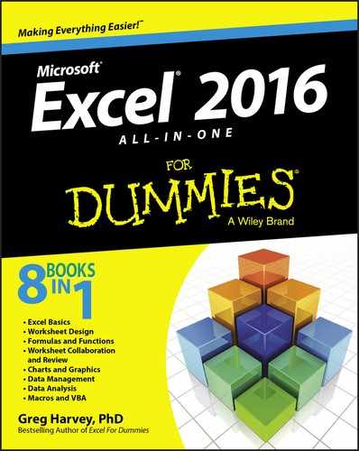
When you first open a new, blank workbook, Excel 2016 opens up a single worksheet (with the generic name, Sheet1) in a new workbook file (with the generic filename, Book1) inside a program window such as the one shown in Figure 1-2.
Figure 1-2: The Excel 2016 program window as it appears after first opening a blank workbook when both Ribbon tabs and commands are displayed.
The Excel program window containing this worksheet of the workbook is made up of the following components:
- File tab: When clicked, this tab opens the Backstage view, which contains a bunch of file-related options including Info, New, Open, Save, Save As, Print, Share, Export, Publish, Close, and Account, as well as Options, which enables you to change Excel’s default settings.
- Quick Access toolbar: You can click the Save, Undo, and Redo buttons to perform common tasks to save your work and undo and redo editing changes. You can also click the Customize Quick Access Toolbar button to the immediate right of the Redo button to open a drop-down menu containing additional common commands such as New, Open, Quick Print, and so on, as well as to customize the toolbar, change its position, and minimize the Ribbon.
- Ribbon: Most Excel commands are contained on the Ribbon. They are arranged into a series of tabs ranging from Home through View.
- Formula bar: This displays the address of the current cell along with the contents of that cell.
- Worksheet area: This area contains all the cells of the current worksheet identified by column headings, which use letters along the top, and row headings, which use numbers along the left edge, with tabs for selecting new worksheets. You use a horizontal scroll bar on the bottom to move left and right through the sheet and a vertical scroll bar on the right edge to move up and down through the sheet.
- Status bar: This bar keeps you informed of the program’s current mode and any special keys you engage, and it enables you to select a new worksheet view and to zoom in and out on the worksheet.
 When using Excel 2016 on a touchscreen device, the Ribbon Display Options are automatically set to Tabs (so that associated commands appear only when you tap a tab) and the Quick Access toolbar contains a Touch/Mouse Mode button. Tap this button followed by the Touch option on its drop-down menu to spread out the tabs and their command buttons on the Ribbon. That way you have a fighting chance of correctly selecting them with your finger or stylus. On a touchscreen tablet such as the Microsoft Surface 3 tablet, an Ink Tools tab where you can modify settings for using a stylus follows the View tab.
Going behind the scenes to Excel’s Backstage view
At the top of the Excel 2016 program window, immediately below the Excel program button and the Save button on the Quick Access toolbar, you find the File menu button (the green one with “File” in white letters to the immediate left of the Home tab).
When you click the File menu button, the Excel Backstage view appears. The screen in this view contains a menu of file-related options running down a column on the left side and, depending upon which option is selected, some panels containing both at-a-glance information and further command options.
At first glance, the File menu button may appear to you like a Ribbon tab — especially in light of its rectangular shape and location immediately left of the Ribbon’s initial Home tab. Keep in mind, however, that this important file control is technically a command button that, when clicked, leads directly to a totally new, nonworksheet screen with the Backstage view. This screen has its own menu options but contains no Ribbon command buttons whatsoever.
After you click the File menu button to switch to the Backstage view, you can then select the Back button (with the left-pointing arrow) that appears above the Info menu item to return to the normal worksheet view or you can simply press the Esc key.
Getting the lowdown on the Info screen
When you choose File ⇒ Info at the top of File menu in the Backstage view, an Info screen similar to the one shown in Figure 1-3 appears.
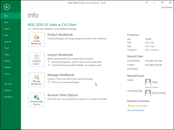
Figure 1-3: The Excel Backstage view displaying the Info screen with permissions, distribution, version commands, and more.
On the left side of this Info screen, you find the following four command buttons:
- Protect Workbook to encrypt the Excel workbook file with a password, protect its contents, or verify the contents of the file with a digital signature (see Book IV, Chapters 1 and 3 for more on protecting and signing your workbooks)
- Inspect Workbook to inspect the document for hidden metadata (data about the file) and check the file’s accessibility for folks with disabilities and compatibility with earlier versions of Excel (see Book IV, Chapter 3 for details on using this feature)
- Manage Workbook to recover or delete draft versions saved with Excel’s AutoRecover feature (see Book II, Chapter 1 for more on using AutoRecover)
- Browser View Options to control what parts of the Excel workbook can be viewed and edited by users who view it online on the Web
On the right side of the Info screen, you see a list of various and sundry bits of information about the file:
- Properties lists the Size of the file as well as any Title, Tags, and Categories (to help identify the file when doing a search for the workbook) assigned to it. To edit or add to the Title, Tags, or Categories properties, click the appropriate text box and begin typing. To add or change additional file properties, including the Company, Comments, and Status properties, click the Properties drop-down button and then select Show Document Panel or Advanced Properties from its drop-down menu. Select Show Document Panel to open the Document panel in the regular worksheet window where you can edit properties such as Author, Title, Subject, and Keywords and to add comments. Select the Advanced Properties option to open the workbook’s Properties dialog box (with its General, Summary, Statistics, Contents, and Custom tabs) to change and review a ton of file properties.
- Related Dates lists the date the file was Last Modified, Created, and Printed.
- Related People lists the name of the workbook’s author as well as the name of the person who last modified the file. To add an author to the workbook file, click the Add an Author link that appears beneath the name of the current author. If the workbook file is new and you’ve never saved it on disk, the words “Not Saved Yet” appear after Last Modified By.
- The Open File Location check box appears under the Related Documents heading. Select it to open the folder containing the current workbook file, where you can find associated workbook files to work with.
- The Show All Properties link, when clicked, expands the list of Properties to include text fields for Comments, Template, Status, Categories, Subject, Hyperlink Base, and Company that you can edit.
Sizing up other File menu options
Immediately below the Info option at the very top of the File menu, you find the commands you commonly need for working with Excel workbook files, such as creating new workbook files as well as opening, saving, and closing files. (See Book II, Chapter 1 for more on saving and closing files and Book II, Chapter 3 for more on opening them.)
The New command immediately below Info displays a New screen, which, just like the Excel Start screen, displays a thumbnail list of all the available spreadsheet templates. (See Book II, Chapter 1 for more on creating and using workbook templates.)
Beneath the Save As command you find the Print option that, when selected, displays a Print screen. This screen contains the document’s current print settings (that you can modify) on the left side and a preview area that shows you the pages of the printed worksheet report. (See Book II, Chapter 5 for more on printing worksheets using the Print Settings panel in the Backstage view.)
Below the Print command you find the Share option, which displays a list of commands for sharing your workbook files online. Beneath this, you find an Export option used to open the Export screen, where you find options for converting your workbooks to other file types as well as controlling the browsing options when the workbook is viewed online in a web browser. (See Book IV, Chapter 4 for more about sharing workbook files online as well as converting them to other file formats.)
The new Publish option enables you to save your Excel workbooks to a folder on your OneDrive for Business account and then publish it to Microsoft’s Power BI (Business Information) stand-alone application that enables you to create visual dashboards that highlight and help explain the story behind the worksheet data.
Checking user and product information on the Account screen
Below the Close option that is used to close a workbook file (hopefully, after saving all your edits) on the File menu, you find the Account option. You can use this option to review account-related information on the Backstage Account screen. When displayed, the Account screen gives you both user and product information.
On the left side of the Account screen, your user information appears, including all the online services to which you’re currently connected. These services include social media sites such as Facebook, Twitter, and LinkedIn, as well as the more corporate services such as your OneDrive, SharePoint team site, and Office 365 account.
To add an online service to this list, click the Add a Service button at the bottom and select the service to add on the Images & Videos, Storage, and Sharing continuation menus. To manage which accounts appear on the list, highlight the name and click the Remove button to take it off the list. To manage the settings for a particular service, click the Manage button and then edit the settings online.
Use the Office Background drop-down list box that appears between your user information and the Connected Services list on the Account screen to change the pattern that appears in the background of the title bar of all your Office 2016 programs. By default, Office 2016 uses a Clouds pattern. You can change the background by selecting a new pattern from the Office Background drop-down menu on the Excel Account screen or have no pattern displayed by selecting None from the menu. Below this option, you see the Office Theme selection (Colorful by default) that sets the overall color pattern you use. Just be aware that any change you make here affects the title areas of all the Office 2016 programs you run on your device (not just the Excel 2016 program window).
On the right side of the Account screen, you find the Product information. Here you can see the activation status of your Office programs as well as review the version number of Excel that is installed on your device. Because many Office 365 licenses allow up to five installations of Office 2016 on different devices (desktop computer, laptop, Windows tablet, and smartphone, for example), you can select the Show Additional Licensing Information link and then click the Manage Account link that appears to go online. There, you can check how many Office installations you still have available and, if need be, manage the devices on which Office 2016 is activated.
Ripping through the Ribbon
The Ribbon (shown in Figure 1-4) groups related commands together with the goal of showing you all the most commonly used options needed to perform a particular Excel task.
Figure 1-4: Excel’s Ribbon consists of a series of tabs containing command buttons arranged into different groups.
The Ribbon is made up of the following components:
- Tabs: Excel’s main tasks are brought together and display all the commands commonly needed to perform that core task.
- Groups: Related command buttons can be organized into subtasks normally performed as part of the tab’s larger core task.
- Command buttons: Within each group you find command buttons that you can select to perform a particular action or to open a gallery. Note that many command buttons on certain tabs of the Excel Ribbon are organized into mini-toolbars with related settings.
- Dialog Box launcher: This button is located in the lower-right corner of certain groups and opens a dialog box containing a bunch of additional options you can select.
To get more of the Worksheet area displayed in the program window, you can minimize the Ribbon so that only its tabs are displayed. (In fact, this Tabs display option is the default setting for Excel 2016 running on a touchscreen device, such as the Microsoft Surface tablet.)
You can minimize the Ribbon by doing any of the following:
- Click the Collapse the Ribbon button (the button with the caret symbol in the lower-right corner of the Excel Ribbon).
- Double-click a Ribbon tab.
- Press Ctrl+F1.
- Click the Shows Tabs item on the Ribbon Display Options button’s drop-down menu.
To redisplay the entire Ribbon and keep all the command buttons on the selected tab displayed in the program window, click the tab and then select the Pin the Ribbon button (the one with the push-pin icon that replaces the Unpin the Ribbon button). You can also do this by double-clicking one of the tabs or pressing Ctrl+F1 a second time, or even by selecting the Show Tabs and Commands item on the drop-down menu that appears when you click or tap the Ribbon Display Options button.
When you work in Excel with the Ribbon minimized, the Ribbon expands each time you select one of its tabs to show its command buttons, but that tab stays open only until you select one of its command buttons. The moment you select a command button, Excel immediately minimizes the Ribbon again so that only the tabs display.
Note, however, that when Excel expands a tab on the collapsed Ribbon, the Ribbon tab overlaps the top of the worksheet, obscuring the header with the column letters as well as the first couple of rows of the worksheet itself. This setup can make it a little harder to work when the Ribbon commands you’re selecting pertain to data in these first rows of the worksheet. For example, if you’re centering a title entered in cell A1 across several columns to the right with the Merge & Center command button on the Home tab, you can’t see the result of selecting the button until you once again minimize the Ribbon by selecting a visible cell in the worksheet. If you then decide you don’t like the results or want to further refine the title’s formatting, you need to redisplay the Home tab of the Ribbon once again, which obscures the cells in the top two rows all over again! (The workaround for this is to do most of your formatting with the commands on the mini-bar that appears when you right-click a cell selection so that you don’t have to open the minimized Ribbon at all. See the section on formatting cells with the mini-bar in Book II, Chapter 2 for details.)
Keeping tabs on the Excel Ribbon
The very first time you launch Excel 2016 and open a new workbook, the Ribbon contains the following seven tabs, proceeding from left to right:
- Home: Use this tab when creating, formatting, and editing a spreadsheet. This tab is arranged into the Clipboard, Font, Alignment, Number, Styles, Cells, and Editing groups.
- Insert: Use this tab when adding particular elements (including graphics, pivot tables, charts, hyperlinks, and headers and footers) to a spreadsheet. This tab is arranged into the Tables, Illustrations, Apps, Charts, Reports, Sparklines, Filter, Links, Text, and Symbol groups.
- Page Layout: Use this tab when preparing a spreadsheet for printing or reordering graphics on the sheet. This tab is arranged into the Themes, Page Setup, Scale to Fit, Sheet Options, and Arrange groups.
- Formulas: Use this tab when adding formulas and functions to a spreadsheet or checking a worksheet for formula errors. This tab is arranged into the Function Library, Defined Names, Formula Auditing, and Calculation groups. Note that this tab also contains a Solutions group when you activate certain add-in programs, such as Conditional Sum and Euro Currency Tools — see Book I, Chapter 2 for more on Excel add-ins.
- Data: Use this tab when importing, querying, outlining, and subtotaling the data placed into a worksheet’s data list. This tab is arranged into the Get External Data, Connections, Sort & Filter, Data Tools, and Outline groups. Note that this tab also contains an Analysis group if you activate add-ins, such as the Analysis Toolpak and Solver Add-In — see Book I, Chapter 2 for more on Excel add-ins.
- Review: Use this tab when proofing, protecting, and marking up a spreadsheet for review by others. This tab is arranged into the Proofing, Language, Comments, and Changes groups. Note that this tab also contains an Ink group with a sole Start Inking button if you’re running Excel on a Windows tablet or smartphone or on a laptop or desktop computer that’s equipped with some sort of electronic input tablet.
- View: Use this tab when changing the display of the Worksheet area and the data it contains. This tab is arranged into the Workbook Views, Show, Zoom, Window, and Macros groups.
Although these seven tabs are the standard ones on the Ribbon, they are not the only tabs that can appear in this area. Excel displays contextual tools with their own tab or tabs as long as you’re working on a particular object selected in the worksheet, such as a graphic image you’ve added or a chart or pivot table you’ve created. The name of the contextual tools for the selected object appears immediately above the tab or tabs associated with the tools.
The moment you deselect the object (usually by clicking somewhere on the sheet outside of its boundaries), the contextual tool for that object and all of its tabs immediately disappears from the Ribbon, leaving only the regular tabs — Home, Insert, Page Layout, Formulas, Data, Review, and View — displayed.
Adding the Developer tab to the Ribbon
If you do a lot of work with macros (see Book VIII, Chapter 1) and XML files in Excel, you should add the Developer tab to the Ribbon. This tab contains all the command buttons normally needed to create, play, and edit macros as well as to import and map XML files. To add the Developer tab to the Excel Ribbon, follow these steps:
Click the File menu button followed by the Options item in the Backstage view (Alt+FT).
The Excel Options dialog box opens in the worksheet view.
- Select the Customize Ribbon option in the Excel Options dialog box and then click the Developer check box under Main Tabs in the Customize the Ribbon list box on the right. Click OK to finish.
Selecting with mouse and keyboard
Because Excel 2016 runs on many different types of devices, the most efficient means of selecting Ribbon commands depends not only on the device on which you’re running the program, but on the way that device is equipped as well.
For example, when I use Excel 2016 on my Microsoft 3 Surface tablet with its touch cover (equipped with both keyboard and touchpad) connected, I select commands from the Excel Ribbon more or less the same way I do when running Excel on my Windows desktop computer equipped with a standalone physical keyboard and mouse or on my Windows 10 laptop computer with its built-in physical keyboard and track pad.
However, when I run Excel 2016 on my Surface 3 tablet when the touch cover is not connected, I’m limited to selecting Ribbon commands directly on the touchscreen with my finger or stylus.
The most direct method for selecting Ribbon commands equipped with a physical keyboard and mouse is to click the tab that contains the command button you want and then click that button in its group. For example, to insert an online image into your spreadsheet, you click the Insert tab and then click the Illustrations button followed by the Online Pictures button to open the Insert Pictures dialog box.
The easiest method for selecting commands on the Ribbon — if you know your keyboard at all well — is to press the keyboard’s Alt key and then type the letter of the hot key that appears on the tab you want to select. Excel then displays all the command button hot keys next to their buttons, along with the hot keys for the Dialog Box launchers in any group on that tab. (See Figure 1-5.) To select a command button or Dialog Box launcher, simply type its hot key letter.
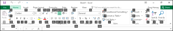
Figure 1-5: When you select a Ribbon tab by pressing Alt plus the hot key assigned to that tab, Excel displays the hot keys for its command buttons.
If you know the old Excel shortcut keys from versions prior to Excel 2007, you can still use them. For example, instead of going through the rigmarole of pressing Alt+HCC to copy a cell selection to the Windows Clipboard and then Alt+HVP to paste it elsewhere in the sheet, you can still press Ctrl+C to copy the selection and then press Ctrl+V when you’re ready to paste it.
Selecting Ribbon commands by touch
When selecting Ribbon commands on a touchscreen device without access to a physical keyboard and mouse or touchpad, you are limited to selecting commands directly by touch.
Before trying to select Excel Ribbon commands by touch, however, you definitely want to turn on touch mode in Excel 2016. You do this by tapping the Touch/Mouse Mode button at the end of the Quick Access toolbar followed by the Touch option on its drop-down menu. When you do this, Excel spreads out the command buttons on the Ribbon tabs by putting more space around them, making it more likely that you’ll actually select the command button you’re tapping with your finger (or even a more slender stylus) instead of the one right next to it. (This is a particular problem with the command buttons in the Font group on the Home tab that enable you to add different attributes to cell entries such as bold, italic, or underlining: They’re so close together when touch mode is not on that they’re almost impossible to correctly select by touch.)
Adjusting to the Quick Access toolbar
When you first begin using Excel 2016, the Quick Access toolbar contains only the following three or four buttons:
- Save: Saves any changes made to the current workbook using the same filename, file format, and location.
- Undo: Undoes the last editing, formatting, or layout change you made.
- Redo: Reapplies the previous editing, formatting, or layout change that you just removed with the Undo button.
- Touch/Mouse Mode (automatically added only to Excel running on touchscreen tablets and computers): Switches between the default mouse mode and touch mode, which puts more space between tabs and their command buttons to facilitate selection with a finger or stylus.
The Quick Access toolbar is very customizable because you can easily add any Ribbon command to it. Moreover, you’re not restricted to adding buttons for just the commands on the Ribbon; you can add any Excel command you want to the toolbar, even the obscure ones that don’t rate an appearance on any of its tabs. (See Book I, Chapter 2 for details on customizing the Quick Access toolbar.)
By default, the Quick Access toolbar appears right above the File Menu button and Ribbon tabs. To display the toolbar beneath the Ribbon above the Formula bar, click the Customize Quick Access Toolbar button (the drop-down button to the direct right of the toolbar with a horizontal bar above a down-pointing triangle) and then select Show Below the Ribbon from its drop-down menu. Doing this helps you avoid crowding out the name of the current workbook that appears to the toolbar’s right.
Fooling around with the Formula bar
The Formula bar displays the cell address and the contents of the current cell. The address of this cell is determined by its column letter(s) followed immediately by the row number, as in cell A1, the very first cell of each worksheet at the intersection of column A and row 1, or cell XFD1048576, the very last of each Excel 2016 worksheet at the intersection of column XFD and row 1048576. The contents of the current cell are determined by the type of entry you make there: text or numbers, if you just enter a heading or particular value, and the nuts and bolts of a formula, if you enter a calculation there.
The Formula bar is divided into three sections:
- Name box: The leftmost section displays the address of the current cell address.
- Formula bar buttons: The second, middle section appears as a rather nondescript button displaying only an indented circle on the left (used to narrow or widen the Name box) with the Insert Function button (labeled fx) on the right until you start making or editing a cell entry. At that time, its Cancel (an X) and its Enter (a check mark) buttons appear in between them.
- Cell contents: The third white area to the immediate right of the Function Wizard button takes up the rest of the bar and expands as necessary to display really, really long cell entries that won’t fit in the normal area. This area contains a Formula Bar button on the far right that enables you to expand its display to show really long formulas that span more than a single row and then to contract the Cell contents area back to its normal single row.
The Cell contents section of the Formula bar is really important because it always shows you the contents of the cell even when the worksheet does not. (When you’re dealing with a formula, Excel displays only the calculated result in the cell in the worksheet and not the formula by which that result is derived.) You can edit the contents of the cell in this area at any time. By the same token, when the Cell contents area is blank, you know that the cell is empty as well.
What’s up with the Worksheet area?
The Worksheet area is where most of the Excel spreadsheet action takes place because it displays the cells in different sections of the current worksheet. Also, inside the cells is where you do all of your spreadsheet data entry and formatting, not to mention the majority of your editing.
Keep in mind that for you to be able to enter or edit data in a cell, that cell must be current. Excel indicates that a cell is current in three ways:
- The cell cursor or pointer — the dark green border surrounding the cell’s entire perimeter — appears in the cell.
- The address of the cell appears in the Name box of the Formula bar.
- The current cell’s column letter(s) and row number are shaded (in an orange color on most monitors) in the column headings and row headings that appear at the top and left of the Worksheet area, respectively.
Moving around the worksheet
Each Excel worksheet contains far too many columns and rows for all of its cells to be displayed at one time. (It’s true: 17,179,869,184 cell totals equal an illegible black blob, regardless of the size of your monitor.) Excel offers many methods for moving the cell cursor around the worksheet to the cell where you want to enter new data or edit existing data:
- Click the desired cell — assuming that the cell is displayed within the section of the sheet currently visible in the Worksheet area.
- Click the Name box, type the address of the desired cell directly into this box, and then press the Enter key.
- Press Alt+HFDG, Ctrl+G or F5 to open the Go To dialog box, type the address of the desired cell into its Reference text box, and then click OK.
- Use the cursor keys, as shown in Table 1-1, to move the cell cursor to the desired cell.
- Use the horizontal and vertical scroll bars at the bottom and right edges of the Worksheet area to move the part of the worksheet that contains the desired cell. Then click the cell to put the cell cursor in it.
Table 1-1 Keystrokes for Moving the Cell Cursor
Keystroke |
Where the Cell Cursor Moves |
→ or Tab |
Cell to the immediate right. |
← or Shift+Tab |
Cell to the immediate left. |
↑ |
Cell up one row. |
↓ |
Cell down one row. |
Home |
Cell in Column A of the current row. |
Ctrl+Home |
First cell (A1) of the worksheet. |
Ctrl+End or End, Home |
Cell in the worksheet at the intersection of the last column that has any Home data in it and the last row that has any data in it (that is, the last cell of the so-called active area of the worksheet). |
PgUp |
Cell one screenful up in the same column. |
PgDn |
Cell one screenful down in the same column. |
Ctrl+→ or End, → |
First occupied cell to the right in the same row that is either preceded or followed by a blank cell. If no cell is occupied, the pointer goes to the cell at the very end of the row. |
Ctrl+← or End, ← |
First occupied cell to the left in the same row that is either preceded or followed by a blank cell. If no cell is occupied, the pointer goes to the cell at the very beginning of the row. |
Ctrl+↑ or End, ↑ |
First occupied cell above in the same column that is either preceded or followed by a blank cell. If no cell is occupied, the pointer goes to the cell at the very top of the column. |
Ctrl+↓ or End, ↓ |
First occupied cell below in the same column that is either preceded or followed by a blank cell. If no cell is occupied, the pointer goes to the cell at the very bottom of the column. |
Ctrl+Page Down |
Last occupied cell in the next worksheet of that workbook. |
Ctrl+Page Up |
Last occupied cell in the previous worksheet of that workbook. |
Note: In the case of those keystrokes that use arrow keys, you must either use the arrows on the cursor keypad or have the Num Lock key disengaged on the numeric keypad of your keyboard.
Keystroke shortcuts for moving the cell cursor
Excel offers a wide variety of keystrokes for moving the cell cursor to a new cell. When you use one of these keystrokes, the program automatically scrolls a new part of the worksheet into view, if this is required to move the cell pointer. In Table 1-1, I summarize these keystrokes and how far each one moves the cell cursor from its starting position.
The keystrokes that combine the Ctrl or End key with an arrow key (listed in Table 1-1) are among the most helpful for moving quickly from one edge to the other in large tables of cell entries. Moving from table to table in a section of the worksheet that contains many blocks of cells is also much easier.
When you use Ctrl and an arrow key to move from edge to edge in a table or between tables in a worksheet on a physical keyboard, you hold down Ctrl while you press one of the four arrow keys (indicated by the + symbol in keystrokes, such as Ctrl+→). On the Touch keyboard, you tap Ctrl and then tap the appropriate arrow key to accomplish the same thing.
When you use End and an arrow-key alternative, you must press and then release the End key before you press the arrow key (indicated by the comma in keystrokes, such as End, →). Pressing and releasing the End key causes the END MODE indicator to appear onscreen in the status bar. This is your sign that Excel is ready for you to press one of the four arrow keys.
Because you can keep the Ctrl key depressed as you press the different arrow keys that you need to use, the Ctrl-plus-arrow key method provides a more fluid method for navigating blocks of cells on a physical keyboard than the End-then-arrow key method. On the Touch keyboard, there is essentially no difference in technique.
You can use the Scroll Lock key to “freeze” the position of the cell pointer in the worksheet so that you can scroll new areas of the worksheet in view with keystrokes such as PgUp (Page Up) and PgDn (Page Down) without changing the cell pointer’s original position (in essence, making these keystrokes work in the same manner as the scroll bars).
After engaging Scroll Lock (often abbreviated ScrLk), when you scroll the worksheet with the keyboard, Excel does not select a new cell while it brings a new section of the worksheet into view. To “unfreeze” the cell pointer when scrolling the worksheet via the keyboard, you just press the Scroll Lock key again.
Tips on using the scroll bars
To understand how scrolling works in Excel, imagine the worksheet is a humongous papyrus scroll attached to rollers on the left and right. To bring into view a new section of a papyrus worksheet that is hidden on the right, you crank the left roller until the section with the cells that you want to see appears. Likewise, to scroll into view a new section of the worksheet that is hidden on the left, you crank the right roller until that section of cells appears.
You can use the horizontal scroll bar at the bottom of the Worksheet area to scroll back and forth through the columns of a worksheet. Likewise, you can use the vertical scroll bar to scroll up and down through its rows. To scroll one column or a row at a time in a particular direction, click the appropriate scroll arrow at the ends of the scroll bar. To jump immediately back to the originally displayed area of the worksheet after scrolling through single columns or rows in this fashion, simply click the darker area in the scroll bar that now appears in front of or after the scroll bar.
You can resize the horizontal scroll bar, making it wider or narrower, by dragging the button that appears to the immediate left of its left scroll arrow. When working in a workbook that contains a whole bunch of worksheets, in widening the horizontal scroll bar you can end up hiding the display of the workbook’s later sheet tabs.
To scroll very quickly through columns or rows of the worksheet, hold down the Shift key and then drag the mouse pointer in the appropriate direction within the scroll bar until the columns or rows that you want to see appear on the screen in the Worksheet area. When you hold down the Shift key as you scroll, the scroll button within the scroll bar becomes really narrow, and a ScreenTip appears next to the scroll bar, keeping you informed of the letter(s) of the columns or the numbers of the rows that you’re currently whizzing through.
If your mouse has a wheel, you can use it to scroll directly through the columns and rows of the worksheet without using the horizontal or vertical scroll bars. Simply position the white-cross mouse pointer in the center of the Worksheet area and then hold down the wheel button of the mouse. When the mouse pointer changes to a four-point arrow, drag the mouse pointer in the appropriate direction (left and right to scroll through columns or up and down to scroll through rows) until the desired column or row comes into view in the Worksheet area.
On a touchscreen, you scroll the worksheet by swiping the screen with your finger. (Don’t use your stylus because pressing it in the worksheet area only results in selecting the cell you touch). You swipe upward to scroll worksheet rows down and swipe down to scroll the rows up. Likewise, you swipe left to scroll columns right and swipe right to scroll columns left.
The only disadvantage to using the scroll bars to move around is that the scroll bars bring only new sections of the worksheet into view — they don’t actually change the position of the cell cursor. If you want to start making entries in the cells in a new area of the worksheet, you still have to remember to select the cell (by clicking it) or the group of cells (by dragging through them) where you want the data to appear before you begin entering the data.
Surfing the sheets in a workbook
Each new workbook you open in Excel 2016 contains a single blank worksheet, aptly named Sheet1, with 16,384 columns and 1,048,576 rows (giving you a truly staggering total of 51,539,607,552 blank cells!). Should you still need more worksheets in your workbook, you can add them simply by clicking the New Sheet button (the circle with the plus sign in it) that appears to the immediate right of Sheet1 tab.
On the left side of the bottom of the Worksheet area, the Sheet tab scroll buttons appear, followed by the actual tabs for the worksheets in your workbook and the New Sheet button. To activate a worksheet for editing, you select it by clicking its sheet tab. Excel lets you know what sheet is active by displaying the sheet name on its tab in green, boldface type as well as underlining the tab and making the tab appear to be connected to the current worksheet above.
Don’t forget the Ctrl+Page Down and Ctrl+Page Up shortcut keys for selecting the next and previous sheets, respectively, in your workbook. You can also click the Next Sheet and Previous Sheet button marked by the ellipsis (…). The Next Sheet button is the one with the ellipsis on the right side of the sheet tabs immediately left of the New Sheet button. The Previous Sheet button is the one with ellipsis on the left side of the sheet tabs to the immediate left of the first visible sheet tab.
If your workbook contains too many sheets for all their tabs to be displayed at the bottom of the Worksheet area, use the Sheet tab scroll buttons to bring new tabs into view (so that you can then click them to activate them). You click the Next Scroll button (the one with the triangle pointing right) to scroll the next hidden sheet tab into view on the right and the Previous Scroll button (the one with the triangle pointing left) to scroll the next hidden sheet into view on the left. You Ctrl+click the Next Scroll button to scroll the last sheet into view and Ctrl+click the Previous Scroll button to scroll the first sheet into view.
Right-click either Sheet tab scroll button to display the Activate dialog box listing the names of all the worksheets in the workbook in their order from first to last. Then, to scroll to and select a worksheet, double-click its name or click the name followed by the OK button.
Taking a tour of the status bar
The status bar is the last component at the very bottom of the Excel program window. (See Figure 1-6.) The status bar contains the following areas:
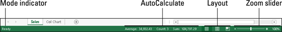
Figure 1-6: The Excel 2016 status bar.
- Mode: This button indicates the current state of the Excel program (READY, ENTER, EDIT, and so on).
- AutoCalculate: This indicator displays the AVERAGE, COUNT, and SUM of all the numerical entries in the current cell selection.
- Layout: This selector enables you to select between three layouts for the Worksheet area: Normal, the default view that shows only the worksheet cells with the column and row headings; Page Layout view, which adds rulers and page margins and shows page breaks for the worksheet; and Page Break Preview, which enables you to adjust the paging of a report.
- Zoom: The Zoom slider enables you to zoom in and out on the cells in the Worksheet area by dragging the slider to the right or left, respectively.
When you begin recording your first macro in Excel 2016 (see Book VIII, Chapter 1 for details), a Stop Recording button (with a square icon) appears on the status bar to the immediate right of the Mode indicator. When you finish recording this macro, the Stop Recording button on the status bar immediately changes into a Record Macro button (using an icon with a dot on a tiny worksheet) that you can thereafter use to record any or all your future macros.
Getting Help
In Excel 2016, help is always available to you in two forms:
- Tell Me help feature that not only shows you the command sequence for the help topic you enter but at times actually initiates and completes the command sequence for you
- Online Help that contains various help topics that explain Excel’s many features
Show-and-tell help with the Tell Me feature
Excel 2016’s new Tell Me help feature must be from Missouri because it doesn’t just tell you what to do; it actually shows you by performing the task for you. This handy little feature is available from the Tell Me What You Want to Do text box located to the immediate right of the last command tab above the Excel ribbon. As you enter a help topic into this text box, Excel displays a list of related Excel commands in a drop-down list.
When you then select one of the items displayed on this list, Excel either selects the associated Ribbon command (no matter which Ribbon tab is currently selected) and waits for you to make a selection from the command’s submenu or, in some case, just goes ahead and completes the associated command sequence for you.
For example, if you type print into the Tell Me What You Want to Do text box, Excel displays a list with the following items:
- Quick Print
- Preview and Print
- Print Preview and Print
- Print Guidelines
- Print Area
- See Help for “Print”
If you select Quick Print at the top of the list, Excel immediately sends the current worksheet to the printer. If, however, you select Preview and Print next on the list, a submenu with Print Preview and Print, Quick Print, and Print Preview Full Screen appears. If you select the Print Preview and Print item, Excel displays a preview of the printout on the Print Screen in the Backstage view that you can print. If you select the Quick Print item, the program sends the worksheet directly to the printer. But if you select the Print Preview Full Screen item, Excel replaces the Worksheet view with a full screen print preview page from which you can print the worksheet. (See Chapter 5 for complete details on previewing and printing your worksheets.)
On the other hand, if you type underline in the Tell Me What You Want to Do text box, Excel displays two items: Underline and See Help for “Underline.” If you then select the Underline item, Excel goes ahead and assigns the underlining font attribute to whatever is in the cell that’s current in the worksheet.
If you would rather learn how to complete a task in Excel rather than have the program do it for you, select the See Help for “xyz” item at the end of the list below the Tell Me What You Want to Do text box. This opens an Excel Help window with loads of information about using the commands to accomplish that task (as described in the very next section).
Using the Excel online help
Excel 2016 offers extensive online help that you can make use of anytime while using the program. To display the Excel Help window, you press function key F1. When you do, an Excel 2016 Help window similar to the one shown in Figure 1-7 appears.
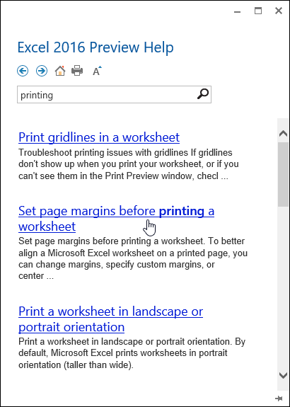
Figure 1-7: The Excel 2016 Help window with help topics for on printing worksheets.
On a device without any access to the function keys, you can display the online Excel 2016 Help window by typing help into the Tell Me What You Want to Do text box and then tapping the Get Help on “help” option in the drop-down list.
This window contains a search text box with a Search button to the right (with the spyglass icon) below a group of command buttons (Back, Next, Home, Print, and Increase Font). To display a list of related help topics in the Help window, type a keyword or name of a category (such as printing, formulas, and so on) and then click the Search button or press Enter. The Excel 2016 Help window then displays a list of help topics for that category. To display detailed information about a particular help topic in this list, click its link.
To print the contents of the help topic that you select, click the Print button (the one with the Printer icon) at the top of the Excel Help window. To return to the opening Excel Help screen, click the Home button. To return to the previous Help screen after reviewing several links in a row, click the Back button (the one with arrow pointing left).
Launching and Quitting Excel
Excel 2016 runs under both the older Windows 7 and 8 as well as the new Windows 10 operating systems. Although the basic procedure for launching Excel 2016 in all three versions of the Windows operating system is pretty much the same, due to the variations to the Windows desktop, you should consult the Excel startup sequence for your particular version of Windows, which I outline in the following sections.
Starting Excel from the Windows 10 Start menu
Windows 10 brings back the good old Start menu that many of you remember from much earlier Windows versions. The Windows 10 Start menu combines the straight up menu from earlier days with the tile icons so prominent in Windows 8. To open this menu to launch Excel 2016, click the Windows icon on the taskbar or press the Windows key on your keyboard.
Then, click the All Apps button under the list of the Most Used applications in the menu and scroll down to Microsoft Office 2016 under the E’s in the list. Select the Expand button (with the caret pointing downward) to display your Office applications where you click Excel 2016, as shown in Figure 1-8.
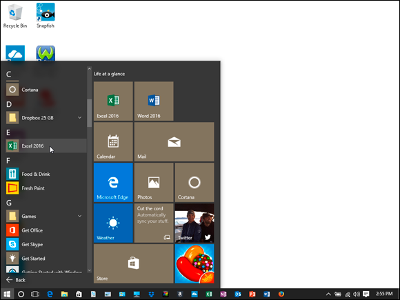
Figure 1-8: Launching Excel 2016 from the Windows 10 Start screen.
You can pin an Excel 2016 button to the Windows 10 Start menu and/or its taskbar so that you can launch Excel simply by selecting this button. To pin a button, right-click the Excel 2016 menu item in the Start menu and then select the Pin to Start and/or Pin to Taskbar items in the displayed context menu.
Starting Excel from the Windows 10 Ask Me Anything text box
Instead of opening the Windows 10 Start menu and locating the Excel 2016 item there, you can launch the program by selecting this item from the Ask Me Anything text box. Simply type excel into this text box that appears to the immediate right of the Windows button on the taskbar and click Excel 2016 at the top of its result list.
Telling Cortana to Start Excel 2016 for you
If you want Cortana, the voice-activated online Windows 10 assistant, to launch Excel 2016 for you, click the microphone icon in the Ask Me Anything text box and then when she displays the listening prompt, say “Cortana, start Microsoft Excel 2016.”
Starting Excel from the Windows 8 Start screen
When starting Excel 2016 from the Windows 8 Start screen, you simply select the Excel 2016 program tile either by clicking it if you have a mouse available or tapping it with your finger or stylus if you’re running Windows 8 on a touchscreen device.
If you can’t locate the Excel 2016 tile among those displayed on the Start screen, use the Search feature to find the application and pin it to the Windows 8 Start screen:
From the Start screen, begin typing exc on your physical or Touch keyboard.
Windows 8 displays Excel 2016 in the list of programs under Apps on the left side of the screen.
Right-click the Excel 2016 button in the Apps list on the left side of the screen.
On a touchscreen device, the equivalent to the right-click of the mouse is to tap and hold the Excel 2016 menu item until a circle appears around your finger or stylus. Then, when you remove your finger or stylus from the screen, the shortcut menu appears.
- Select the Pin to Start option from the menu bar that appears at the bottom of the screen.
After pinning an Excel 2016 tile to the Windows 8 Start screen, you can move it by dragging and dropping it in your desired block.
Starting Excel from the Windows 7 Start menu
When starting Excel 2016 from the Windows 7 Start menu, you follow these simple steps:
Click the Start button on the Windows taskbar to open the Windows Start menu.
To select the Start button on a device equipped with a mouse, you click the button. To select the Start button on a touchscreen device with no mouse or touchpad, you tap the button on the touchscreen.
- Choose All Programs from the Start menu, choose Microsoft Office 2016, and then choose Excel 2016.
You can use the Search Programs and Files search box on the Windows 7 Start menu to locate Excel on your computer and launch the program in no time at all:
- Click the Start button on the Windows 7 taskbar to open the Windows Start menu.
Select the Start menu’s search text box and type the letters exc to have Windows locate Microsoft Office Excel 2016 on your computer.
If you’re using a device without a physical keyboard, double-tap the right edge of the Touch keyboard that appears on the left edge of the Windows Start menu and screen to make the entire keyboard appear and then tap out the letters exc.
- Select the Microsoft Excel 2016 option that now appears in the left Programs column on the Start menu.
Pinning Excel to the Windows 7 Start menu
If you use Excel all the time, you may want to make its program option a permanent part of the Windows 7 Start menu. To do this, pin the program option to the Start menu:
Start Excel from the Windows Start menu.
To launch Excel, use the appropriate method for your version of Windows, as I outline earlier in this chapter.
After launching Excel, Windows adds Microsoft Office 2010 to the recently used portion on the left side of the Windows Start menu.
- Click the Start menu and then right-click Microsoft Office Excel 2016 to open its shortcut menu.
- Choose Pin to Start Menu from the shortcut menu.
After pinning Excel in this manner, the Microsoft Office Excel 2016 option always appears in the upper section of the left column of the Start menu. You can now launch Excel simply by clicking the Start button and then clicking this option.
Pinning Excel to the Windows 7 taskbar
If your computer runs Windows 7, you can add a Microsoft Excel 2016 icon to the standard Internet Explorer, Windows Explorer, and Windows Media Player buttons on its taskbar.
To do this, drag the Microsoft Excel 2016 icon that you’ve either pinned to the Windows Start menu (see “Pinning Excel to the Windows 7 Start menu,” which immediately precedes this section) or that you’ve added as a shortcut to the Windows desktop and drag and drop it into its desired position on the Windows 7 taskbar.
After you pin a Microsoft Excel 2016 icon to the Windows 7 taskbar, the button appears on the Windows taskbar each time you start your computer, and you can launch the Excel program simply by single-clicking its Quick Launch button.
When it’s quitting time
When you’re ready to call it a day and quit Excel, you have several choices for shutting down the program:
- Press Alt+FX or Alt+F4 on your physical or Touch keyboard.
- Select the Close button (the one with the x) in the upper-right corner of the Excel program window.
- Click the Excel program button (the green one with the x on a partially opened book to the immediate left of the Save button on the Quick Access toolbar) followed by the Close option on its drop-down menu.
If you try to exit Excel after working on a workbook and you haven’t saved your latest changes, the program beeps at you and displays an alert box querying whether you want to save your changes. To save your changes before exiting, click the Yes command button. (For detailed information on saving documents, see Book I, Chapter 2.) If you’ve just been playing around in the worksheet and don’t want to save your changes, you can abandon the document by clicking the No button.