
Chapter 3
Quantifying Uncertainty
Robert F. Bordley
Integrated Systems & Design, University of Michigan, Ann Arbor, MI, USA; Defense & Intelligence Group, Booz Allen Hamilton, Troy, MI, USA
Laplace: The theory of probability is at bottom nothing but commonsense reduced to calculus.
3.1 Sources of Uncertainty in Systems Engineering
Best practice in systems engineering identifies all relevant factors outside the control of the design team. Some of these factors, for example, certain external interfaces, are completely known to the team. But “many phenomena that are treated as deterministic or certain are, in fact, uncertain,” (OMB guidance, circular 94, 2015). The inappropriate treatment of uncertain quantities as deterministic, also called the flaw of averages (Savage et al., 2012), can lead to design decisions that could prove very costly if the actual value of this quantity is very different from the average. So the team must acknowledge their uncertainty about both
- what is feasible and affordable, for example, technological, integration, interface, and supply uncertainties and
- what is desirable, for example, uncertainties about stakeholder preferences, adversary reactions, and environmental changes impacting stakeholders and adversaries.
There is added intrateam uncertainty due to different specialists within the design team not knowing how they will be impacted by the choices and discoveries of other specialists.
In addition to acknowledging these uncertainties, the team must continuously update their understanding of these uncertainties as they learn more information. Information about uncertainties can be learned from risk management activities that address both
- uncertainty about outcomes and
- the severity of the consequences associated with outcomes.
Since these two dimensions addressed by risk management are typically but not always (Bordley & Hazen, 1991) unrelated, this section only focuses on outcome uncertainty.
3.2 The Rules of Probability and Human Intuition
Probability theory was created (Bernstein, 1998) by mathematicians (Galileo, Pascal, Cardano) working as consultants to affluent gamblers. The uncertainties gamblers address in gambling houses as illustrated in Figure 3.1 are generated from analog mechanisms such as spinning roulette wheels, rolling dice, dealing out playing cards, and, in modern times, digital mechanisms such as random number generation software operating on embedded microprocessors. While the gambler may not understand these mechanisms, the owners of the gambling house (or their consultants) do understand these mechanisms. These uncertainties have several convenient properties:
- All of the possible outcomes of the gambling device (e.g., all of the possible outcomes of spinning a roulette wheel) are known.
- There are a set of elementary outcomes (e.g., the slots in the roulette wheel or a number on the roll of a single die) that are equally likely.
- The outcome of one trial of a gambling device (one roll of a die) is independent of the outcome of a second trial of a gambling device.

Figure 3.1 Uncertainty in gambling
Uncertainties that are analogous to the uncertainties arising from gambling devices (such as rolling a dice) are often called aleatory uncertainties from the Latin word for dice.
Because of these properties, the aleatory probability of a gambler winning a bet equals the fraction of elementary outcomes consistent with the gambler winning the bet. If a gamble is played repeatedly, then this fraction eventually reflects the long-run frequency with which different outcomes will occur. This makes this fraction useful in developing long-run strategies for both gamblers and gambling houses.
All the equally likely outcomes of the gambling device can be arranged as points on a square. Each of these points represents a different “state” of the world. Suppose that some of these outcomes, if they occur, would be acceptable to the systems engineer's stakeholders. Draw a circle labeled A around the acceptable stakeholder outcomes (and let Ac denote the set of remaining unacceptable outcomes).
Suppose an engineering test was conducted with certain outcomes passing the test and others not passing the test. While satisfying stakeholders is the goal of the systems engineer, passing the test is often the goal of a supplier to the systems engineer. Draw a circle labeled E about the outcomes passing the engineering test (with Ec denoting the outcomes outside the circle that fail the test). Then the problem can be represented with the classic Venn diagram shown in Figure 3.2.
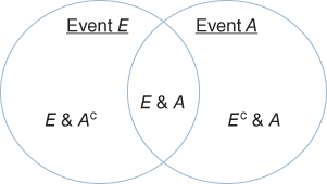
Figure 3.2 Venn diagram
If E and A include exactly the same points, then an outcome that failed the engineering test would also be unacceptable to users (and vice versa). In reality, there will be some outcomes, E&Ac, that pass the engineering tests but are unacceptable to stakeholders as well as outcomes, Ec&A, that fail the engineering tests but are acceptable to stakeholders.
Note that P(E&A) can never exceed P(E). While this is obvious from the Venn diagram, psychological experiments establish that human intuition often violates this principle. For example, in one such experiment, individuals were asked to estimate the probability of a very liberal individual either being a bank teller or being a feminist bank teller, that is, being both a feminist and a bank teller. Individuals consistently judged being a feminist bank teller as more likely than being a bank teller (Tversky & Kahneman, 1974). So in this example, human intuition was in error.
Since all outcomes are treated as equally likely, the proportion of outcomes passing the engineering test will equal the probability, P(E), that the engineering test is passed. Since the sum of the proportion of outcomes passing the test and the proportion of outcomes not passing the test is 1, P(E)+P(Ec)=1. Also note that summing
- the proportion of outcomes passing the test that are acceptable to stakeholders
- the proportion of outcomes passing the test that are not acceptable to stakeholders
gives the proportion of outcomes passing the test. As a result,
This seems obvious from the Venn diagram in Figure 3.2. But psychological evidence shows that human intuition often violates this principle. In another psychological experiment,
- a group of individuals estimated the probability of death from natural causes
- a second group estimated the probability of death from heart disease, the probability of death from cancer, and the probability of death from a natural cause other than heart disease or cancer.
Summing up the probabilities from this second group consistently gives a higher probability of death than probability assessed by the first group (Tversky & Koehler, 1994). So once again, human intuition was found to be in error.
Define ![]() ) and
) and ![]() . Then
. Then
Of those outcomes passing the engineering test, the quantity P(A|E) corresponds to the proportion that is also acceptable to stakeholders. If P(A|E) = P(A|Ec), then
In this case, events A and E are independent where independence is defined as follows.
- Independence: Events A and E are called independent if P(A) = P(A|E), that is, if knowing that the occurrence of outcome in E does not alter the probability of occurrence of an outcome in A.
When events A and E are independent, both P(A|E) = P(A) and P(E|A)=P(E). But events are typically not independent. Specifically,
Since P(E) = P(E|A)P(A)+P(E|Ac)P(Ac), substituting for P(E) gives an expression known as Bayes' rule:
- Bayes' rule:

If an unacceptable outcome always fails the engineering test (and P(E|Ac)=0), then P(A|E) = 1.
When P(E|Ac) is nonzero, then one can define the likelihood ratio L(A;E) = P(E|A)/P(E|Ac) as a measure of how much the probability of passing the test differs between acceptable and unacceptable outcomes. Then Bayes' rule can be rewritten as
When L(A;E) = 1 (and the test does not discriminate between acceptable and unacceptable outcomes), P(A|E) = P(A), that is, the test result is independent of whether an outcome is acceptable. But as L(A;E) increases (with P(A) positive), P(A|E) increases.
According to equation 3.4, P(A|E) will only equal P(E|A) when P(A)=P(E). So even if the test was very discriminating with P(E|A)=1 and P(E|Ac)=0.05 (and L(A;E) = 20), no conclusion could be drawn about P(A|E) until P(A) was specified. But experimentation shows that people typically treat P(A|E) as equaling P(E|A) without considering the value of P(A) (Villejoubert & Mandel, 2002). So human intuition would interpret a positive test result as indicating that event A is likely to be true. This has led to very serious errors both in medicine (where patients were diagnosed as having cancer based on a test result) and in legal cases (where defendants were judged guilty based on circumstantial evidence).
To show why P(A|E) does not always equal P(E|A), suppose that P(A) = 1%, that is, the probability of a randomly chosen outcome satisfying the stakeholders is quite small. If there are 2000 possible outcomes, then
- 1% of 2000 or 20 of these outcomes will be acceptable
- If the test is administered to all 2000 outcomes, then all 20 of the acceptable outcomes pass the test.
- 99% of 2000 or 1980 outcomes will be unacceptable
- If the test is administered to all 2000 outcomes, then 5% of the 1980 unacceptable outcomes (or 99 unacceptable outcomes) pass the test.
So 20 + 99 = 119 outcomes would pass the test if it were administered to all 2000 outcomes. Since only 20 of these 199 outcomes are acceptable, the probability of an outcome being acceptable given it passed the test, or P(A|E), is approximately 20/119 = 17%. Thus, an outcome passing the test is still unlikely to meet stakeholder expectations. This example shows that both L(A;E) and P(A) must be specified to determine P(E|A). For historical reasons, the probability P(A) is commonly called the prior probability while P(A|E) is called the posterior probability.
These rules of probability can be derived from Kolmogorov's three axioms (Billingsley, 2012):
- (A1) Suppose E1, …, En are disjoint events, that is, at most, one of these events can occur. Then,
3.6

- (A2) If U is an event that includes all possible outcomes, then P(U) = 1.
- (A3) For any event E, P(E) ≥ 0.
For example, equation 3.1 can be deduced from (A1) by defining E1 = E&A and E2 = E&Ac. While these axioms simply formalize commonsense, this section highlighted three cases where informal commonsense contradicted the rules implied by these axioms. Because human intuition about probability is often misleading, careful, and consistent calculation of probabilities is critical in properly accounting for uncertainty.
3.3 Probability Distributions
3.3.1 Calculating Probabilities from Experiments
When a gambler makes a wager (e.g., places a bet on odd numbers appearing on the roulette wheel), the gambler is running an experiment where the outcomes of the experiment are payoffs, that is, how much money the gambler wins or loses. By repeatedly placing a wager and comparing the results with repeated use of different wagers, the gambler generates statistics useful in evaluating the payoffs from different gambling strategies. All the results of interest are easily measured and all the possible outcomes of the experiment (called the experimental sample space) are known in advance.
But while the gambler can make the same wager over and over again, there are many realistic settings where it is not possible to repeat the same decision under the same circumstances. Furthermore, even if it were possible to repeat the same decision, it might not be possible to measure the resulting outcomes of this repeated decision. So the conditions that hold in a gambling house do not necessarily hold in realistic settings. Fortunately, new concepts and measurement devices had been invented, which allowed these conditions to be approximately satisfied in settings outside the gambling house. These inventions allowed probability to be applied across a wide variety of scientific and engineering contexts. As Laplace wrote, “it is remarkable that a science which began with the consideration of games of chance should have become the most important object of human knowledge.”
Scientific experiments typically involve the comparison of experimental treatments with control treatments on the dimension of interest. Making these comparisons is considerably easier when the dimension is an ordinal scale where objects can be ranked from low to high. There are many ways to create an ordinal scale. The Mohs scratch test scale (Hodge & McKay, 1934) ranks the hardness of rocks based on which rock can scratch which other rock. Thus, diamond ranks higher than quartz (because diamond can scratch quartz) while quartz ranks higher than gypsum because quartz can scratch gypsum.
For illustrative purposes, suppose the experimental group consists of belted drivers and the control group consists of unbelted drivers. Let the ordinal dimension of interest be the injuries sustained in collisions. Then all possible outcomes of both treatments can be ranked. Suppose that in this ranking, minor injuries outrank moderate injuries and moderate injuries outrank major injuries. This immediately gives a ranking of any treatment guaranteed to lead to only one outcome. To rank other treatments, define the state of an accident by the kind of vehicles involved in the collision, vehicle speeds, and other factors. Suppose the following property holds.
- State-Wise Dominance: For each possible state, the outcome of the experiment treatment never ranked lower (and, in at least one case, ranked higher) than the outcome of the reference treatment.
When this property holds, the experimental treatment outranks the control treatment.
But in the seatbelt example, state-wise dominance does not hold because there are some states, for example, a burning or submerged vehicle, in which belted drivers may have greater injuries than unbelted drivers. To introduce a more generally applicable notion of dominance, define P0(X) as the probability of the reference treatment leading to outcome x and P1(X) as the probability of the experimental treatment leading to outcome x. Also define the cumulative probability as
- Cumulative Probability: The cumulative probability, F1(x), is the probability of the experimental treatment leading to an outcome ranked no higher than x. This probability is defined over all possible outcomes x in the sample space.
We similarly define F0(x) as the probability of the reference treatment scoring no better than x. Suppose the following statistics were collected.
Table 3.1 includes injuries from cars burning, being submerged, and other accidents.
Table 3.1 Distribution of Injuries From a Major Accident
| Treatment | Minor Injuries (%) | Moderate Injuries (%) | Severe Injuries (%) |
| Belted | 30 | 20 | 10 |
| Unbelted | 10 | 10 | 60 |
Since being unbelted leads to fewer minor or moderate injuries than being belted, being belted does not state-wise dominate being unbelted. But note the following:
- For severe injuries, F1(severe) = 10% < F0(severe) = 60%.
- For moderate to severe injuries, F1(moderate) = 30% < F0(moderate) = 70%.
- For minor to severe injuries, F1(minor) = 60% < F0(minor) = 80%.
So the probability of having a less severe injury (i.e., an outcome ranked higher) is greater for belted drivers. We can formalize this property as follows.
- Stochastic Dominance: For any reference outcome t, the probability of the experimental treatment leading to an outcome outranking outcome t is at least as high as the probability of the control treatment leading to an outcome outranking outcome t (i.e., F1(t) < F0(t) for all t).
If the experimental treatment were state-wise dominant with respect to the control treatment, then it would be stochastically dominant. But while stochastic dominance will in general allow more treatments to be ranked than state-wise dominance, it still does not allow all possible treatments to be ranked.
To rank a treatment in the absence of stochastic dominance, the American Psychological Association mandated (Wilkinson & Task Force on Statistical Inference, 1999) the use of the effect size measure (which is different from the widely known measure of statistical significance). The simplest and most general formulation of the effect size measure (McGraw & Wong, 1992; Grissom & Kim, 2011) is the probability of the experimental treatment leading to an outcome outranking the outcome of the control treatment.
To describe the effect size measure, define X1 (and X0) as a random variable leading to outcome x with probability P1(x) (and P0(x)) for all possible outcomes x. The experiment treatment's effect size is the probability that X1 outranks X0. If there are m experimental treatments numbered k = 1,…,m, then treatment k's effect size is defined as the probability that Xk outranks X0 – where each experimental treatment k is compared with the control treatment. The experimental treatments can be compared with one another based on their effect size. If Pk(x) is the kth treatment's probability of leading to outcome x, then the kth treatment's effect size is ∑x F0(x) Pk(x), that is, the expected probability of outranking the control treatment on the dimension of interest.
3.3.2 Calculating Complex Probabilities from Simpler Probabilities
Applying these concepts requires that F(x) be specified. Sometimes the probability for a complex event can be estimated from known probabilities for simpler events. For example, suppose the probability of a single component failing in some time period is prespecified as equaling r. Suppose there are two components in a system, each with this same probability of failure. Also, suppose that the components are independent. Then there are several possible outcomes:
- Both components could fail. This occurs with probability r2.
- Only one component remains functional. This will occur if either
- the first component fails while the second remains functional. This will happen with probability r(1 − r) or
- the second component fails while the first remains functional. This will happen with probability (1 − r)r.
So the overall probability of only one component being functional is 2r(1 − r).
- Both components could remain functional. This occurs with probability (1 − r)2.
This specifies the probability of two, one, and zero failures in the system.
In the more general case of a system with N components, calculating the probability of x components failing (and (N − x) remaining functional) requires listing the number of distinct outcomes consistent with exactly x components failing. This includes such outcomes as follows:
- The first x components fail while the last N − x components remain functional.
- The first (N − x) components remain functional while the last x components fail.
Let C(N,x) be the number of possible distinct outcomes (or permutations) where exactly x out of N components fail. The probability of each of these outcomes occurring is rx(1 − r)N−x. Hence, the total probability of any of these outcomes occurring, P(x), is described by the following.
- The Binomial Distribution:

If the system only fails when at least x out of N components fail, the probability of the system not failing, that is, having x − 1 failures or fewer, will be F(x − 1).
Using the binomial distribution is difficult when N is very large (e.g., greater than 100). But instead of treating r as a parameter whose value is fixed, suppose the expected number of failures, a = r N, is treated as fixed. Then for large N and a small (e.g., a < 20), the binomial distribution can be approximated by the simpler Poisson distribution. Because the Poisson distribution allows N to be continuous, the Poisson distribution can be used to estimate the number of failures occurring over some time interval N.
The probability of zero failures in time interval N in the Poisson is ![]() . So the probability that the time until the first failure exceeds N is
. So the probability that the time until the first failure exceeds N is ![]() . Thus, the Poisson distribution for discrete outcomes also implies a distribution (referred to as the exponential distribution) over the continuous variable N. This distribution will be a building block for some of the distributions considered in the next section.
. Thus, the Poisson distribution for discrete outcomes also implies a distribution (referred to as the exponential distribution) over the continuous variable N. This distribution will be a building block for some of the distributions considered in the next section.
3.3.3 Calculating Probabilities Using Parametric Distributions
When x is large (or continuous), estimating F(x) can be difficult. As a result, it is convenient to define F(x) so that it is completely specified by a small number of parameters. While there are many possible functions, statistical practice has identified a small number of basic distribution functions F(x) that provide the flexibility needed to address a wide variety of practical problems. In complex problems, the actual function F(x) may have to be written as a weighted average (or mixture) of these basic distribution functions.
These basic distribution functions are completely specified by a location parameter, M, and a scaling parameter, s. There are three kinds of basic distribution functions:
- Unbounded. In this case, the value of the uncertain variable x has neither a lower bound nor an upper bound. The location parameter equals the expected value (or mean) of x while the scaling parameter equals the standard deviation of x.
- Bounded from below. In this case, the value of x has a lower bound but no upper bound. The scaling parameter will still equal the standard deviation, but the location parameter now equals the lower bound. (If x has an upper bound but no lower bound, redefining F to be a function of −x allows the uncertainty to be treated as if it were bounded from below.)
- Bounded from above and below. In this case, the value of x has both a lower and an upper bound. The location parameter will equal the lower bound, but the scaling parameter now equals the difference between the upper and lower bounds.
Once M and s are identified, define the standardized value of x by ![]() and the standardized distribution by
and the standardized distribution by ![]() .
.
In the unbounded case, F*(r) is assumed to be the normal distribution (Figure 3.3) whose values are available in look-up tables:
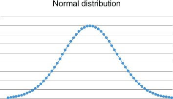
Figure 3.3 Normal distribution
According to the central limit theorem, the normal distribution describes the average of many independent and identically distributed errors (when the mean and variance of these errors are finite.) In applications where the normal distribution understates the degree to which extreme outcomes or black swans (Taleb, 2007) occur, the t or Cauchy distribution may be used instead.
In the case where there is a lower bound on x but no upper bound, F(r) is often assumed to follow the Weibull distribution (Figure 3.4).
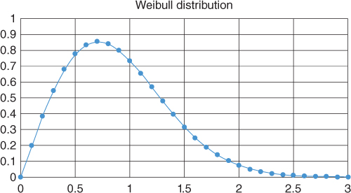
Figure 3.4 Weibull distribution
In some cases, the Gamma, Fréchet, or lognormal distributions are used instead of the Weibull distribution. The shape of these distributions is similar to the shape of the Weibull distribution.
If there are both a lower bound and an upper bound on x, it is common to assume that F*(r) is the beta distribution (Figure 3.5):
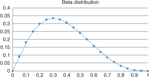
Figure 3.5 Beta distribution
The beta distribution requires the specification of two parameters (in addition to the lower and upper bounds.) In project management applications where only a single parameter, that is, the best estimate of x, is specified, the Beta Pert distribution is used. The Beta Pert distribution corresponds to a Beta distribution where the Beta distribution parameters are set to yield an expression for the variance used in the PERT scheduling tool. As an alternative to either the Beta distribution or the Beta Pert distribution, some practitioners use the more easily explained triangular distribution (Figure 3.6):
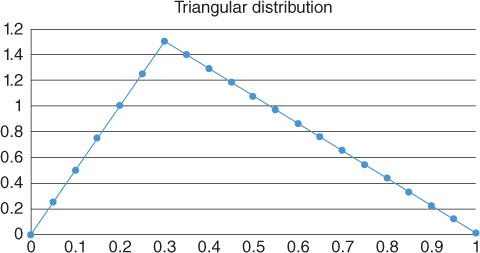
Figure 3.6 Triangular distribution
The analytic expressions for these distributions are given in Table 3.2.
Table 3.2 Distributions and Their Parameters and Functions
| Name | Variable | First Parameter | Second Parameter | P(x) | Mean | Application |
| Binomial | x | a: Probability of success | N: # successes & failures | N!/[x!(N − x)!] ax(1 − a)N−x C(x,N − x) = N!/[x!(N − x)!] |
Na | Discrete # successes in discrete time |
| Poisson | x | a: Mean successes | exp(−a) ax/x! | a | Discrete # of successes in continuous time | |
| Standardized normal | r = (x − M)/s | (1/2π)1/2 exp(−r2/2) | 0 | Continuous unbounded variable | ||
| Standardized Weibull | r = (x − M)/s | a: Shape parameter | a ra−1 exp(−ra) | Gamma function at (1+1/a) | Continuous variable with only a lower bound | |
| Standardized beta | r = (x − M)/s | a: Success parameter | b: Failure parameter | ra−1 (1−r)b−1C(a − 1,b − 1) C(a,b) = (a+b)!/[a!b!] |
a/(a+b) | Continuous variable with upper and lower bound |
| Standard triangular | r = (x − M)/s | a: Best estimate | 2r/a for r < a, 2(1 − r)/(1 − a) for r > a |
(1 + a)/3 | Continuous variable with upper and lower bound |
These and other distributions are compactly described in the classic textbook of Johnson et al., (1995).
3.3.4 Applications of Parametric Probability Distributions
- Application of the Gaussian Distribution: System validation is concerned with ensuring that stakeholders are truly satisfied with the system when they use it. Suppose the systems engineer develops a design that is used to create several products that are sold to different customers. To satisfy these customers, the systems engineer must consider two kinds of variability:
- Variability in the quality of the different units of product created from the design.
- Variability in the level of quality expected by different customers. For example, customers driving on cold snowy roads place very different demands on their car than customers driving in a dry hot desert.
The customer will only be satisfied when the quality of the product purchased by the customer meets or exceeds that customer's expectations (Bordley, 2001).
If x is the difference between product quality and customer expectations, the customer will be satisfied when x > 0. If Q is the mean quality customers expect and q is the mean quality the system provides, then the mean of X is M = q − Q. Let V be the variance of the quality customers expect, and let v be the variance in the quality the system provides. If product quality is uncorrelated with customer expectations, the variance of x will be v + V with s being the square root of that variance. Since the customer is satisfied when x > 0 and since r = (x − M)/s, the customer will be satisfied when r > −M/s. In order to maximize the number of satisfied customers, the engineer will maximize (M/s).
Improving mean quality q will always improve (M/s). But note the following:
- If M > 0, reducing product variability will improve (M/s) and thus customer satisfaction.
- If M < 0, reducing product variability reduces (M/s) and thus customer satisfaction.
Hence, contrary to intuition, reducing variability can reduce customer satisfaction if M = q − Q < 0, that is, if the product's mean quality is less than the customer's mean expectations.
- Application of the Weibull Distribution: A core problem in systems engineer is decomposing a system requirement into subsystem requirements. For example, suppose the systems engineer must assign targets t and t* to two engineering teams. The systems engineer is uncertain about the following:
- Whether or not each engineering team can achieve these targets. If the target is more than the team can achieve, then the project fails. But if the target is less than what the team can achieve, the team will only deliver the target level of performance.
- Whether or not the combined output, t + t*, will satisfy stakeholder needs. If the output fails to satisfy stakeholder needs, the project fails.
Let x and x* represent the uncertain amount each team can deliver, and let X represent what the stakeholder will expect when the system is finished. Then to maximize the probability of setting targets, which are both achievable and acceptable to the stakeholder, t and t* should be chosen to maximize the joint probability
3.7
which is the product of three probabilities.
To solve this problem (Bordley & Pollock, 2012), let s and s* be the standard deviations describing the uncertain performance of the first and the second team, respectively. Let M and M* be the lower bounds on what the first and the second team, respectively, can achieve.
Define r = [(x − M)/s] to be the standardized performance of the first team, and define r* = [(x* − M)/s*] to be the standardized performance of the second team. Then the objective function can be rewritten as
3.8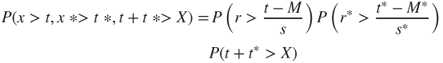
Suppose the systems engineer can also specify an upper bound, U, on how demanding customer expectations might be. The quantity (U − X) describes the uncertain amount by which actual stakeholder expectations will be less stringent than U. The systems engineer describes the likelihood of (U −X) being less stringent than the most extreme expectations by specifying a scaling factor S. The scaling factor may partially reflect the systems engineer's confidence in how well customer expectations have been managed. Define R = [(U − X)/S]. Then the objective function can be further rewritten as
3.9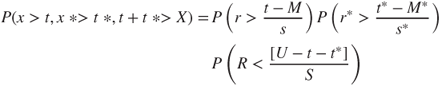
If r, r*, and R are described by Weibull distributions, calculus can be used to solve for the values of t and t* maximizing this probability. In this solution, both t and t* will be proportional to U–M–M*, which corresponds to the maximum gap between customer expectations and the worst-case product performances. As a result, the solution assigns each team responsibility for making up some fraction of the maximum gap. Because there is some possibility that customer expectations will not be as stringent as U, the teams will not be required to make up all of the gap.
- Application of the Beta Distribution: Define the reliability of a supplier to the project as the supplier's probability, r, of producing a part meeting design specifications. Suppose the reliability of this supplier is unknown but the historical reliability of other suppliers is known. Suppose the fraction of those other suppliers having a reliability of r is proportional to a beta distribution P(r) with parameters a and b. If we have no reason to believe that the project's supplier is systematically better or worse than these other suppliers, it may be reasonable to assume that this supplier is comparable to a supplier randomly drawn from this population. Given this assumption, the probability of the supplier having a reliability of r can be described by a beta distribution with parameters a and b.
The supplier is asked to produce a small batch of n parts. The parts are tested, and k of these products are found to meet specifications while the other (n − k) do not. The probability of observing this test result, if the reliability of the supplier were r, is given by a binomial probability P(k|r,n). Given this information, the original probability P(r) can be updated using Bayes' rule to
3.10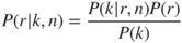
Substituting for the binomial and beta distribution implies that P(r|k,n) is proportional to
3.11
which is a beta distribution with parameters a* = a + k and b* = b + n − k. So the new information has not changed the fact that r is described by a beta distribution. It has only changed the value of the parameters. This parameter change adjusts the probability of one of the supplier's part meeting specification from E[r] = a/(a + b) to E[r|k,n] = a*/(a*+b*). Defining w = n/(a + b + n) implies
3.12
As a result, the revised probability of the supplier's part meeting specifications, E[r|k,n], is a weighted average of the frequency, f, estimated from experiment and the probability of meeting specifications, E[r], based on the population of factories. See Raiffa and Schlaifer (1961) for a classic discussion of this and other updating formulas.
3.4 Estimating Probabilities
3.4.1 Using Historical Data
Note that
As n increases, w increases toward 1, and the value of E[r|k,n], which initially equals E[r], increasingly approximates the empirical frequency. So E[r|k,n] is an adjustment of the empirical frequency, f, to a value closer to some reference value E[r]. If E[r|k,n] had equaled f, it would be an unbiased estimate – since it does not systematically deviate from the empirical data. Instead, it is an estimator that is based on “shrinking” the distance between the unbiased estimator and some reference value. Such a biased estimator is called a shrinkage estimator (Sclove, 1968). While bias is typically considered undesirable, the mean squared error of an estimate is the sum of the square of the bias in an estimator and variance. Hence, a shrinkage estimator could outperform a biased estimator if it had a lower variance, which more than offset the square of its bias. Such shrinkage estimators have been designed and validated in many applications, for example, marketing (Ni, 2007), where sample sizes are limited.
The shrinkage estimator, E[r|k,n], had updated parameter values a* = a + k and b* = b + n − k. Because k and n −k represent actual observations of success and failure, it is common to refer to the parameters a and b as being pseudo-observations of success and failure with a* and b* being the sum of actual and pseudo-observations.
OMB guidance writes that, “in analyzing uncertain data, objective estimates of probabilities should be used whenever possible.” Consistent with this guidance, empirical Bayes methods (Casella, 1985) estimate the prior probability (and, in this case, a and b) from the empirical frequencies in some larger population of systems similar to the system of interest. If the system of interest were a new vehicle program, then the parameters a and b of the prior probability might be estimated by calculating the mean and standard deviation of failure rates for past vehicles made by that manufacturer. If there were N observations in this database of similar systems, then E[r|k,n] combines the n observations from the experiment with the N historical observations of similar systems. Since the N observations are used to generate (a + b) pseudo-observations, the average historical observation is given a weight of w = (a + b)/N relative to each of the experimental observations.
Sometimes there are several choices for the historical population, for example,
- a historical population of vehicles made by the same manufacturer;
- a larger historical population of all vehicles made by any American manufacturer; and
- a still larger historical population of vehicles made by any manufacturer.
Suppose we treat these populations as subpopulations of one large population. If we were to randomly pick a system – comparable to the system of interest – from this large population, it would be important to use stratified sampling in order to increase the probability of sampling from more similar subpopulations and decrease the probability of sampling from less similar subpopulations. If a weight is assigned to each subpopulation reflecting the similarity between that subpopulation and the system of interest, this stratified sampling would effectively weight observations from similar subpopulations more than observations from less similar subpopulation – consistent with the concept of similarity-weighted frequencies (Billot et al., 2005). This use of information from all the subpopulations, instead of just the most similar subpopulation, is consistent with the general finding (Poole & Raftery, 2000) that combining multiple different forecasts of an event yields more accurate predictions than using the best of any one of the forecasts (Armstrong, 2001).
Thus, the prior probability can be used to incorporate historical data on both very similar and less similar systems. The importance of incorporating such information was highlighted by the catastrophic failure of the Space Shuttle Challenger. Recognizing that the Space Shuttle was a uniquely sophisticated system, NASA had estimated its failure rate as extremely low using a sophisticated version of the fault tree methods. But when the failure occurred, this estimated failure rate seemed unrealistic. As the Appendix (Feynman, 1996) to the Congressional commission space shuttle catastrophe report noted, the historical frequency with which failures occurred in general satellite launches would have provided a considerably more realistic estimate of failure rate – even though the shuttle is very different from a satellite. These findings suggest that even though some systems engineering projects (e.g., the space shuttle, the Boston Big Dig, the first electric vehicle, first catamaran combat ship, complex software packages) are truly one-of-a-kind systems, historical data on less similar systems can still be helpful. In fact, Lovallo & Kaheman (2003) argued that forecasts of a project's completion time based on the historical completion time frequency of somewhat similar projects were considerably more realistic than model-based forecasts, which considered only important details about the project and ignored the historical information about the past, less similar projects.
While this section focused on updating beta probabilities, these same convenient updating rules can be generalized (Andersen, 2015) to apply to the larger “exponential” family of distributions. The exponential family of distributions includes most (but not all) of the probability distributions used in engineering, for example, the normal, gamma distribution, chi-squared, beta, Dirichlet, categorical, Poisson, Wishart and inverse Wishart distributions, the Weibull (when the shape parameter is fixed), and the multinomial distribution (when the number of trials is fixed). In these more general distributions, k is replaced by a vector of sufficient statistics, that is, statistics that describe all the information in the n observations relevant to the model parameters.
The generalizability of this updating rule across so many different probability distributions has motivated the definition of the Bayesian average as the sum of actual and pseudo values divided by the number of actual and pseudo-observations.
3.4.2 Using Human Judgment
The previous section discussed procedures for assessing prior probabilities from historical information. But suppose there is no historical information. To determine how to specify the prior probability, consider an analyst using prior probabilities to create a probability model that will be presented to the systems engineer. The systems engineer will then use this model to make various decisions. Consider the following two scenarios:
- The results of this probability model were never shown to the engineers. As a result, the engineers relied on their experiences and intuitions to make decisions. Since these are the decisions the engineers would make prior to receiving new information, we refer to these decisions as the “default decisions.”
- The probability model was shown to the engineers. But the engineers felt that none of the information used by the probability model was credible. Furthermore, sensitivity analysis showed that the recommendations of the model were very sensitive to the inputs provided to that model. Consistent with the Garbage-In/Garbage-Out (GIGO) Principle, the engineers rejected the model. The engineers then made the default decisions (Figure 3.7).

Figure 3.7 Default decision
In many applications, the default decisions involve continuing with current plans and not making any changes. In addition to being consistent with the Hippocratic dictum (Bordley, 2009) of “doing no harm,” avoiding change may also be the most legally defensible course of action. In these applications, different systems engineers will agree on the default decisions. But in other applications, the default decisions may vary depending upon which systems engineer is making the decisions. In other words, the default decision depends upon the experiences and intuitions of the decision-maker. This potential subjectivity in the default decision highlights the importance of having experienced systems engineer with good intuition.
If the model is not credible, then these default decisions will be appropriate – as long as they were made rationally. If a rational decision is a decision satisfying the Bayesian axioms of rationality (Savage, 1954), then the default decisions will be consistent with the decisions supported by some hypothetical probability model where the prior probability in this model is equal to what is often called the personal probability. This personal probability, such as the default decision, can vary from engineer to engineer.
Since the default decisions are the appropriate decisions in this case, the analyst can ensure that the model leads to the appropriate decision by setting the prior probability equal to this personal probability. The model will then reproduce what the engineer would do if there were no credible data. If the model does have credible information, then the posterior probability implied by the model will update that personal probability based on that credible information.
For example, suppose an engineer will do nothing unless the probability of an innovation succeeding exceeds 95%. Then the engineer's personal probability of the innovation succeeding is less than 95%. But in this case, as in most cases, knowing the default decisions typically does not give the analyst sufficient information to specify the personal probability. As Abbas (2015) suggests, probabilities might be chosen to maximize entropy subject to those probabilities being consistent with various decisions. But even if the analyst uses maximum entropy arguments, the analyst will typically need more information on what decisions the engineer would make in other related decision situations. To gather this information, the analyst may present the engineer with hypothetical choice experiments and observe the engineer's response.
To illustrate these hypothetical choice experiments, consider a simpler situation where the analyst wants to assess the prior probability of some event occurring. Then in a typical experiment, the analyst asks a subject matter expert (SME) to choose between
- winning money by betting on the event of interest occurring. (If we are trying to assess a cumulative probability distribution F(x), then the event of interest might be observing an uncertain value exceeding some threshold x) and
- winning money by betting on a casino gamble where the chance of payoff is known to be some stated probability P.
In this simple situation, the SME will always have a clear preference for either betting on the event or betting on the casino gamble unless P is set equal to the probability of the event occurring. Hence, by running this experiment with enough values of P, we can determine the personal probability. To minimize the number of experiments needed, the analyst typically begins with P = 0.5, observe the SME's decision and
- if the SME had decided to bet on the event, define the next experiment using a larger value of P (e.g., P = 0.75)
- if the SME had decided to be on the casino gamble, define the next experiment using a smaller value of P (e.g., P = 0.25).
These stated preference experiments are typically (Wardman, 1988) regarded as less reliable than revealed preference experiments in which individuals actually make a prior choice and receive a payoff (vs stating what they would have chosen); however, revealed preferences are not available in situations when there no analogues from the past. When there is substantial data, the probability will closely approximate historical frequencies (Gelman et al., 2013) and the prior probabilities will become irrelevant (as long as the default probabilities do not equal 0 or 1). Decades of psychological research has focused on improved ways of estimating personal probabilities from such experiments (Lichtenstein et al., 1982).
3.4.3 Biases in Judgment
In a gambling house, the probabilities are calibrated, that is, the asymptotic frequency with which an event occurs will equal the probability it is assigned. But there is no physical mechanism ensuring that this will be the case with personal probabilities. In fact, there is substantial empirical evidence indicating that personal probabilities are systematically biased. For example, probabilities are often based on what people can remember and human memory is systematically biased toward remembering more vivid events at the expense of less memorable events (Lichtenstein et al., 1978). Since individuals will want their personal probabilities to be as calibrated as possible, they will revise their personal probabilities if they are given evidence that they are poorly calibrated.
This willingness to revise a probability has important practical implications for systems safety engineering and, in particular, on the amount of system safety achievable with redundant components. Consider a system that is designed to fail only when 10 different components simultaneously fail. Let A1, …, A10 denote the events of failure of components 1, …, 10, respectively. Suppose these systems are causally independent, that is, the factors that would cause one system to fail are completely unrelated to the factors that would cause another system to fail. Then it is common to assume that these components are statistically independent so that the chance of the system failing is the product of P(A1), …, P(A10). For simplicity, suppose that each component has an identical probability r = (1/2) of failing. Then the chance of failure is roughly 1 in 1000. This calculation is valid for aleatory probabilities where r represents a long-run frequency.
But suppose these probabilities are personal probabilities. Then the expert will be uncertain about the actual long-run frequency corresponding to the probability r. Suppose this uncertainty about r is described, as before, with a beta distribution. In this beta distribution, let the parameters a = b = 1 so that P(r) is a constant, that is, all values of r are equally likely. This is called a uniform distribution and is sometimes interpreted as representing ignorance. The mean value of r is E[r] = 1/(1+1). As a result, P(A1),…, P(A10) = (1/2) as before.
Now suppose the first component fails. This failure gives the expert information about the realism of their personal probabilities. Using the rule for updating the beta distribution, the parameters of the beta distribution describing the expert's beliefs change to a = 2, b = 1. This implies that the probability of failure (the mean value of r) is now 2/(2 + 1) = (2/3). In other words, P(A2|A1) = (2/3), which is unequal to P(A2) = (1/2). As a result, A1 and A2 are not statistically independent (Harrison, 1977). Hence, events that are causally independent need not be statistically independent if their probabilities are assessed by a common measurement device (in this case, the expert), which has some unknown level of bias.
Now suppose that the first two components fail. Then the parameters of the beta distribution change to a = 3, b = 1. As a result, P(A3|A1 A2) = (3/4). The same argument can be used to show that P(Ak|A1, …, Ak−1) = (k/(k + 1)). Hence, the joint probability of all 10 components failing is
The probability of a system with 10 redundant components failing – in the presence of uncertain measurement bias – is now approximately 10%. This is two orders of magnitude greater than the estimated chance of failure when all probabilities were calibrated.
This phenomenon would only be a serious problem if individuals were well-calibrated. Unfortunately, the empirical evidence establishes that individuals are, in fact, poorly calibrated. This is hardly surprising. As the celebrated psychologist Amos Tversky noted, having an individual assess the probability of an event is at least as hard as having a navigator estimate the distance to the shore in a dense fog. Experienced navigators are better at estimating than inexperienced individuals. The same is also true for probability assessment. Weather forecasters are very well-calibrated, that is, roughly 20% of the events to which they assign probability P = 0.20 are eventually found to occur (and 80% do not occur), 40% of the events to which they assign probability P = 0.4 occur, and so on. This stimulated research on training individuals to become better probability assessors. This research has resulted in formal probability assessment training and certification programs (Hubbard, 2010).
One of the first steps in becoming a calibrated probability assessor is to understand the biases, which can distort probability assessments. There are many different kinds of bias, for example,
- Motivational Bias. The most qualified expert on whether a research project will be successful is often the people working on the project. But these individuals know that assigning pessimistic probabilities to their project succeeding could lead to its cancellation – which jeopardizes the funding of themselves or their colleagues. So the most qualified expert will also have the greatest difficulty being objective. Instead of asking the expert to assess a probability, the expert should be asked to provide specific details on what they have accomplished on the project and what remains to be accomplished in order for the project to be a success. This can allow a comparison of progress of the project with other projects whose probability of success might be known. This approach is implemented in NASA's technology readiness level system (El-Khoury & Kenley, 2014).
- Anchoring and adjustment bias. Suppose we are defining the lower, upper, and most likely values as part of assessing probabilities for continuous events. It has been found that individuals – if first asked to specify a most likely value – will then estimate the lower and upper bounds by adjusting that most likely value. This typically leads to lower and upper bounds that are unrealistically close to the best estimate. To avoid this bias, the lower and upper bounds should be estimated before providing a best estimate.
- Overconfidence in making assessments. To address this bias when individuals have estimated a lower bound, ask individuals to think about scenarios in which the true value might be lower than this lower bound. This often motivates them to further downwardly adjust their estimate to obtain a more realistic lower bound. Similarly, when individuals have made a tentative estimate of an upper bound, they should be asked to think of scenarios where values could be higher than this upper bound. Only when individuals are satisfied with their lower and upper bounds, should they be asked to specify a most likely value.
These biases – as well as other previously discussed biases – have been documented in more than half a century of psychological work, which was recognized by Daniel Kahneman, who received the Nobel Prize in 2002 (Flyvbjerg, 2006).
The Kolmogorov axioms (Billingsley, 2012) were enunciated to describe the aleatory uncertainties generated by randomization mechanisms (such as gambling devices) whose properties were well understood. But there are also epistemic uncertainties reflecting the lack of knowledge about the mechanisms (Kiurehgian & Ditlevsen, 2009) themselves. These biases in intuition occur regardless of whether the uncertainties are aleatory or epistemic. (There are also biases that only occur with epistemic probabilities (Ellsberg, 1961).)
This motivates using probability to remedy the biases associated with both aleatory and epistemic uncertainties. In fact, the Bayesian axioms of rationality require the use of probability for modeling all uncertainties. However, fuzzy set theory (Zimmermann, 2001) and Dempster–Shafer theory (Shafer, 1976) have been used as alternatives to probability theory for reasoning on epistemic uncertainties. Since most scientists and engineers are familiar with probability theory, this book uses probability theory to describe all uncertainties. This also allows the use of the Bayesian axioms of rationality as a unifying foundation for all the techniques discussed in this chapter.
3.5 Modeling Using Probability
3.5.1 Bayes Nets
The available information is often not captured in a manner that is adequate to make an informed decision. Fortunately, the rules of probability can be useful in converting the available information into the information that is adequate for making decisions. Converting this information requires us to exploit the interdependencies between the events about which we have information and the events on which we need to have information. Because of the sheer number of events and the complexity of the relationships involved, graphical representations can be quite useful.
- Bayes Nets: Bayes nets (Pearl, 2000) are a graphical representation of the probabilistic interdependencies between events.
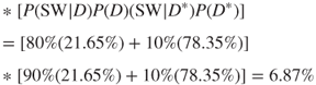
Bayes nets (Ben-Gai, 2007) are extremely useful in converting whatever information happens to be available into the information needed to make informed engineering decisions. For example, consider a warning system for a military base (Figure 3.8). There is a measurement device that is sensitive to the movements of adversaries and animals. Let P(B) = 20% be the probability of a bear being in the vicinity, let P(A) = 5% be the probability of an adversary being in the vicinity, and assume that these two events are probabilistically independent. Let P(D|B) = 50% be the probability of the measurement device detecting motion given there is an animal, let P(D|A) = 90% being the probability given an adversary, let P(D|B&A) = 95% when both are present, and let P(D|B*&A*) = 0 when neither are present. If movement is detected, there is a visual warning (VW) system providing a warning with probability P(VW|D) = 80% and a sound system providing a warning with a probability P(SW|D) = 90%. Suppose there is a probability P(VW|D*) = P(SW|D*) of both systems given warnings when no motion is detected. We can represent this problem graphically:

Figure 3.8 Bayes net example
The absence of an arc connecting Adversary and Animal in the Bayes Net is a representation of the assumption that the two events are independent, that is, the probability of both occurring is given by
The probability that the device detects motion using the law of total probability is

Note that while arcs connect the two events, sound warning (SW) and VW, to the detection event (D), no arcs connect SW or VW to either A and B. So once the outcome of D is known, the occurrence of either a VW or a SW will be independent of whether or not there was an animal or adversary. As a result,
Also, note that there is no arc connecting VW to SW. As a result, the events VW and SW are assumed to be conditionally independent – given movement is detected (D) and also given it is undetected (D*), that is,
To show that VW and SW, while being conditionally independent, are not unconditionally independent, we compute the probability of occurrence of both the VW and SW as
We now show that P(VW & SW) > P(VW)*P(SW) by computing
VW and SW are not independent because both warnings depend upon whether or not the detector was triggered.
This graphical representation allows for the computation of the joint probability of the events: SW, VW, D, B, and A. If the joint probability is known, then all the probabilities associated with any combination of these events can also be calculated. For example, it is possible to calculate the probability of an adversary, but not an animal being present, given there was a VW. Since these probabilities are based on the technologies used in designing the detectors and warning systems, they may change if these technologies were replaced with newer technologies. As a result, the Bayes net could be used to specify how different technologies change the probability of soldiers being warned given an adversary is present as well as the probability of a false alarm (the probability of soldiers being warned when an adversary is not presented). When rectangular nodes corresponding to the choice of technologies (and other decisions) are explicitly added to the Bayes net, the Bayes net becomes an influence diagram (Shachter, 1986).
3.5.2 Monte Carlo Simulation
In deterministic modeling, a mathematical or physical model is constructed, which calculates the variables of interest from input variables with known values in a certain setting. The model is calibrated by testing to ensure that it gives the correct answers for settings where both the input and output values are known. If the input values are uncertain but we know the probability distribution of the input values, then the parameters of the distribution of output variables (e.g., the expected value and the variance) can sometimes be calculated. But if there are many input variables or the functional form of the input–output model is not restricted to relatively simple, closed forms such as linear and quadratic equations, then the exact calculation of expected values and variances is very difficult. (This is the curse of dimensionality and nonlinearity.) In fact, if the model is complex enough, calculating output parameters from a small number of input parameters can be very difficult.
To address this computational problem, we return once again to the gambling house context, which was the motivation behind probability theory. Instead of developing a model relating input parameters to output parameters, this procedure only uses the original deterministic model relating input values to output values.
Suppose we are trying to estimate the maximum velocity of a boat through the water. This will typically depend on the length, width (beam), depth (draft), and weight of the boat as well as the temperature, turbulence, and many other aspects of the water. Since the equations required to calculate the resistance of the water to the boat are notoriously complicated – and usually require test data – closed-form solutions are generally not feasible. To estimate velocity with the simplest version of the Monte Carlo process, assume that our input random variables Xk are independent and have a known probability distribution F(Xk). In this case, the Monte Carlo process
- uses random number generators to generate n independent and uniformly distributed random variables (U1, …, Un) ;
- assigns the ith input variable value x1 for which F(xi) = ui for i = 1,…, n;
- uses the model to calculate an output value y1 from these input values;
- stores these values for the ith iteration in a table and repeats step 1 until the desired number of iterations has been implemented.
By the central limit theorem, the mean of the frequency distribution of the output values in the table will approximate the normal distribution with a variance inversely proportional to the number of parameters. As a result, the sample mean and variance will then give us the desired parameters of the approximate output distribution of mean of the outputs (see Figure 3.9).
Figure 3.9 Monte Carlo simulation
In realistic settings, it is important to consider four refinements of this approach.
3.5.3 Monte Carlo Simulation with Dependent Uncertainties
To motivate the first refinement, note that the length, width, draft, and weight of a boat were assumed independent. But the weight of the boat will be less than the product of the length, width, draft, and mass density. As a result, the weight is not independent of the length, width, and draft. This shows that it is necessary to allow for dependency between the input variables X1, …, Xn. We now use the following Monte Carlo procedure to generate random variables with the appropriate multivariate distribution.
The Monte Carlo methods generated independent and random values of X1, …, Xn by first generating uniformly and independently distributed values of U1, …, Un. To generate values of X1, …, Xn, which are dependent, we must generate dependent values of U1, …, Un from some multivariate distribution, which describes uniform random variables that are dependent. We denote this multivariate distribution by C(U1, …, Un) where C(U1, …, Un) = U1…Un if the variables are independent and equals min(U1, …, Un) if the variables are perfectly positively dependent. Copula theory (Nelsen, 2007) establishes that C will be that function for which F(X1, …, Xn) = C(F(X1), …, F(Xn)).
Hence, to use Monte Carlo methods when X1, …, Xn are dependent, we first specify the multivariate distribution F(X1, …, Xn) and the univariate distributions F(X1), …, F(Xn), then infer the function C, and then generate the uniform random variables U1, …, Un from the distribution C(U1, …, Un). We then use the ith uniform random variable generated from distribution C to assign a value to xi by setting F(xi) = ui.
3.5.4 Monte Carlo Simulation with Partial Information on Output Values
To motivate the second refinement, suppose the model indicated that our sailing boat would achieve an average maximum speed of 700 knots (which is more than 10 times the world's record.) This unusually high-speed prediction will naturally make us skeptical of either the model or some of the input values used in the model (Kadane, 1992). If we felt the model was accurate and if there were no uncertainty in our input values, then we would simply accept the model's prediction as valid and ignore our initial skepticism. If we were absolutely confident in our information about maximum boat speeds, we would use that information about boat speeds to adjust (or calibrate) our prior input values. But in most cases, we will be uncertain about both inputs and outputs.
This will require a procedure for simultaneously adjusting both input values and output values. Let X denote the uncertain input variables and Y the output variables with P(X,Y) being a prior probability, which is not based on the model but is based on all other judgmental and historical data. Suppose we consider the model without any information on the values of input variables. Then the model only gives us new information about previously unrecognized relationships between the input and output values (Bordley & Bier, 2009). To represent this information, let Y(x) be a random variable describing the possibly uncertain value of y, which the model generates given the input value x.
First, suppose we describe the information from the model by the output of a single simulation run. In this run, random values x1 for each input variable are generated based on our prior beliefs P(X). The model is then used to infer the output value y1 associated with those input values. In the absence of the model, the probability of observing this output value y1 – given the knowledge of X and Y and the input value x1 – would be
As Bordley (2014) proved, this probability is proportional to the likelihood of the model being accurate when the true input and output values are known to be X and Y.
Now suppose we describe the model with m simulation runs. Then (x1,…, xm) represents the m inputs of each of those runs while (y1, …, ym) are the output values which the model associates with these input values. The likelihood of the model would be proportional to
Multiplying the likelihood by P(XY) gives the updated probability for XY given the model. Integration over X then gives the updated probability of Y. When all uncertainties are Gaussian, P(yk|xk,XY) can be written in terms of the probability of deviations between the simulated inputs and true input values leading to some level of deviation between the simulation output and the true output value. In this Gaussian case, the expected value of the output variable will be a weighted average of two forecasts:
- A forecast based on only the model and input information.
- A forecast based on all other (prior) information about the output value.
3.5.5 Variations on Monte Carlo Simulation
Our last two refinements involve more substantive changes to Monte Carlo analysis. To discuss the third refinement, note that each iteration in the standard Monte Carlo process generates a new sequence of input values by randomly drawing from the same input distribution. But sometimes, this input distribution, P(x), is difficult to calculate. Fortunately, there is an alternative approach that allows us to perform this sampling while generating observations using more tractable expressions for the probability distribution.
- Let k = 1. Generate the first value of x = x1 based on some convenient density q(x).
- Define k = k + 1. Generate the value of xk for the kth iteration using the more easily calculated conditional probability p(xk|xk−1).
- Repeat step 2.
Because the value generated in the (k + 1)st iteration only depends on the value generated in the kth iteration, this iterative process forms a Markov chain. For Markov chains, the probability with which xk is generated on the kth iteration will approximate some stationary distribution P(x) for large k – as long as q(x) and P(xk|xk−1) assign nonzero probabilities to all combinations of observations. This Monte Carlo Markov chain approach (Brooks et al., 2011) has been widely used in the recent decades.
For the fourth refinement, note that the Monte Carlo approach randomly selects input values, uses the model to calculate an output value, and then reruns the model for different selections of input values. An alternate approach is to model each single input value as a vector with the components of that vector being randomly selected values for that input. The model could then be applied once to the vector for each input value in order to generate a vector of output values. While a variation of this approach was implicitly implemented in the Analytica Bayes Net software (Morgan & Henrion, 1998), Savage developed a technique for enabling Excel to perform these operations. Unlike the Monte Carlo Markov chain, this technique, called probability management, is a recent new development,which is discussed in more detail in Section 9.5.
3.5.6 Sensitivity Analysis
Logical and physical models are used to model the performance at each higher level as a function of the performance at each lower level. However, we cannot calculate the overall performance without specifying the values for the inputs. While the Monte Carlo method was designed to avoid us having to specify exact values for inputs, we still need to specify a probability distribution for these input values. Since collecting information takes time and resources, a preliminary analysis is performed with very limited information (e.g., with information on only the lower and upper bounds of the input variables.)
Suppose we are interested in determining whether we are at risk of violating our mass target for a vehicle. Vehicle mass is driven by the mass of various subsystems. Suppose there were only three vehicle subsystems, that is, door modules, engine, and body. Suppose we only set a subsystem's mass to its lower or upper bound. This leads to 23 = 8 different combinations of vehicles (Table 3.3).
Table 3.3 Vehicle Mass Combinations
| Run | Door | Engine | Body |
| 1 | Lower Bound | Lower Bound | Lower Bound |
| 2 | Upper Bound | Lower Bound | Lower Bound |
| 3 | Lower Bound | Upper Bound | Lower Bound |
| 4 | Upper Bound | Upper Bound | Lower Bound |
| 5 | Lower Bound | Lower Bound | Upper Bound |
| 6 | Upper Bound | Lower Bound | Upper Bound |
| 7 | Lower Bound | Upper Bound | Upper Bound |
| 8 | Upper Bound | Upper Bound | Upper Bound |
In a full factorial design of experiments (Barrentine, 1999) with two levels, a separate simulation run would be used to calculate vehicle mass for each of these possible combinations. Because there were only three input variables, there were only eight vehicle mass estimates. In the actual application, there were 13 input variables and 8192 (213) different mass estimates. A separate simulation run was used to calculate vehicle mass for each of these possible combinations.
We then pick one input variable, for example, seats.
- In half of the runs (or 4096 cases), seat mass was set to its lower bound. We calculate the average vehicle mass for those classes. This gives us the average vehicle mass given that the seat mass is set to its lower bound.
- In the other half of the runs (or 4096 cases), the seat mass was set to its upper bound. We similarly calculate the average vehicle mass for those cases. This gives us the average vehicle mass given that the seat mass is set to its upper bound.
The difference between the higher and lower of these two numbers gives the variation in vehicle mass associated with variations in seat mass.
We repeat this procedure for each of the input variables and obtain the average vehicle masses when each variable's mass is set to the lower bound and when each variable's mass is set to the upper bound. As Figure 3.10 shows, we then plot the upper and lower vehicle masses associated with each variable – with the highest variation variables plotted at the top of the chart. This chart highlights the variables whose variation has the greatest impact on vehicle mass. The data point at the junction of the light gray bar and the dark gray bar for each variable is the estimate of the expected value using all 8192 (213) estimates.
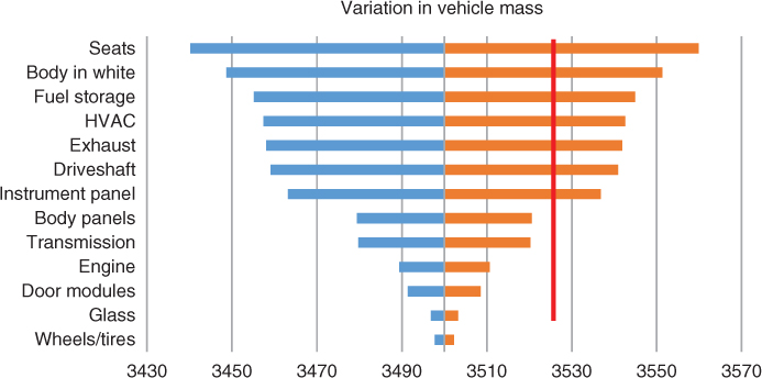
Figure 3.10 Tornado diagram for sensitivity analysis
The chart includes a red line for a mass target, which identifies those variables that could potentially lead to violations in that target. But in some cases, the red line – instead of representing the target – might represent the mass associated with an alternative design. In this case, the seat mass might – if it were known to equal its worst-case estimate – lead us to consider switching to the alternative design. However varying the map of the body panels will not cause us to switch to the alternative design. In fact, the bottom six variables – even if they were set to their upper value – would not change our decision while the top seven variables might. Thus, the sensitivity analysis has identified those variables which could – if we learned more about their actual values – potentially change the decision suggested by a deterministic analysis. This allows attention to be focused on better understanding and quantifying the uncertainty in these two factors – using the methods discussed in this section.
The sensitivity analysis may also be used for a second purpose. Once the critical uncertainties are identified, they can be used to construct a small number of intuitively meaningful scenarios with each scenario reflecting the outcome of the uncertainties assuming various extreme values. These scenarios are communicated to the stakeholders. Use cases can then be constructed, which allow stakeholders to describe how they want the system to behave in the presence of these scenarios.
As noted previously, calculation of these estimated vehicle masses when there are 13 variables requires 8192 observations. When the separate experiment required to generate each observation is time-consuming and costly, performing this analysis may not be cost-effective. Fractional factorial designs (Kulahci & Bisgaard, 2005) provide an ingenious way of conducting the sensitivity analysis with fewer observations.
3.6 Summary
Uncertainty is implicit, although frequently ignored, in many aspects of systems engineering. In reliability-based design optimization (Bordley & Pollock, 2009), the project manager often minimizes two kinds of risks:
- Project Risk: The risk of not satisfying stakeholder expectations.
- Safety Risk: The risk of injury to individuals or damage to property.
While originally developed to describe the uncertainties encountered in gambling, probability is generally applicable to all uncertainties. Because human intuition is easily misled in thinking about uncertainties, systematic use of applied probability is essential. Probabilities should be calculated using
- models to relate the event of interest, Y, to other events, X;
- experimental or field information on past occurrences of Y or X or past occurrences of events partially similar to X or Y;
- judgmental probabilities – collected with psychologically validated elicitation protocols.
Monte Carlo and related techniques allow for the integration of analytical modeling with probability assessments. Sensitivity analysis can then be used to determine which uncertainties have the biggest impact on the outputs of the Monte Carlo model.
3.7 Key Terms
- Anchoring and Adjustment Bias: Psychological tendency to underestimate the range on a variable by anchoring on a single number and then making upward and lower adjustments in that number.
- Bayes Nets: Graphical model specifying each variable using a node with the probabilistic relationship between different variables represented by arcs between different nodes.
- Beta Distributions: Widely used probability distribution for a continuous variable with lower and upper bounds.
- Binomial Distributions: Probability distribution for number of successes in a discrete number of trials.
- Cognitive Biases: Psychologically innate tendencies to deviate from how a rational person would make a decision or describe their beliefs and values about a situation.
- Cumulative Distribution: Probability of a variable being less than some input value x.
- Design of Experiments: A systematic method for specifying the input values to a series of experiments, which extracts the maximum amount of information on quantities of interest.
- Decomposition Bias: A systematic tendency for the sum of the psychologically assessed probability of different events exceeding the psychologically assessed probability of any one of those events occurring.
- Bayes Rule: A rule for calculating the conditional probability of an event given new information from
- the probability of that event and alternative events prior to getting that information
- the likelihood of that information if each of these possible events were true.
- Deterministic Dominance: The value of a random variable is never less (and in some cases exceeds) than that of another random variable.
- Effect Size: A measure of how much the outcome of one treatment differs from the outcome of another.
- Eliciting Probabilities from Experts: A scientific procedure for describing an expert's beliefs about an uncertainty based on the expert's observed responses to different questions or problems.
- Ignoring Base Rate Bias: Assess the probability of an event without considering the probability with which identical (or nearly identical) events have occurred in the past.
- Laws of Probability: An extension of the rules of logic for reasoning about uncertain quantities.
- Monte Carlo Simulation: Technique for calculating the probability distribution of some possibly probabilistic function by repeatedly sampling the input values from probability distributions.
- Motivational Bias: A tendency to assess probabilities so as to favor one's self-interest.
- Normal Distribution: A distribution that – when the number of observations is large – closely approximates the sum of the values assigned to those observations. This distribution is also used to describe the distribution of quantities with no lower or upper bounds.
- Optimism Bias: Tendency to overestimate the probability of desirable events occurring.
- Probability: A measure of a rational individual's willingness to gamble on an event's occurrence.
- Probability Assessment: A probability estimated based on an individual's judgment.
- Redundancy: Deliberately creating multiple components to perform a function that could be achieved by one function. Typically used to increase the probability of that function being performed given the occurrence of unanticipated events.
- System Safety: The probability of a system not leading to unanticipated injury or loss of life.
- Uncertainty: Imperfect knowledge of the value of some variable.
- Representativeness Bias: Estimation of the probability of an observation being drawn from some population based on the degree to which the observation is similar to other units in that population (Kahneman & Tversky, 1972).
- Risk: A potential and undesirable deviation of an outcome from some anticipated value.
- Sensitivity Analysis: A procedure for determining how much a variable of interest changes as a function of changes in the values of other variables.
- Stochastic Dominance: A relationship between two uncertain quantities where the first uncertain quantity never has a smaller probability (and in at least one case, has a better probability) of achieving an outcome ranked higher than the second quantity.
- Triangular Distributions: A popular distribution in which the probability of achieving a higher score increases linearly in that score up to some peak value and then decreases linearly.
- Updating Probabilities Based on Data: A process for revising a probability given new information (data) specified by the rules of probability.
- Weibull Distributions: Popular distribution for describing an uncertainty with a lower bound.
3.8 Exercises
- 3.1 Suppose the probability of a typical project being successful was 40%. Suppose that of those projects which have eventually been successful, 80% of them have had a strong sponsor. In contrast, of those projects which have not eventually been successful, only 40% of them had a strong support.
- a. If your project has a strong sponsor, what is the probability of it being successful?
- b. What is the probability of the typical project having a strong sponsor?
- c. What is the probability your project fails if it does not have a strong sponsor?
- d. Calculate the odds of success (the ratio of the probability of success to the probability of failure) both for a typical project and for a project with a strong sponsor. How much does a strong sponsor change the odds of success? How does this compare with the likelihood ratio?
- 3.2 Suppose your system uses five parts. There is a 5% probability of each part being defective. Part failures are independent.
- a. If your system fails if any part fails, what is the probability of the system failure?
- b. If your system fails if any two parts fail, what is the probability of the system failure?
- c. Suppose the probability of a part failing doubles to 10%. If your system fails when any two parts fail, what is the probability of the system failure?
- d. How do these three probabilities of system failure compare?
- 3.3 Your system will be used for 10 years. The probability of failing at any point in time does not change. The expected number of system failures in the course of 10 years is expected to be 2.
- a. What is the probability of the system having one failure in its lifetime? What is the probability of the system having five failures in its lifetime?
- b. If there are two failures in 10 years, the rate of failure is 1/5. What is the probability of the system not having any failures in 2 years?
- c. What is the expected number of failures in 2 years?
- 3.4 The weight of a component could, once it is designed, range anywhere from 10 pounds to 20 pounds. Your best estimate of the component weight is 12 pounds.
- a. If you assume that the weight follows a triangular distribution, what is the probability of the component weight being less than 15 pounds?
- b. How about if you use assume that the weight follows a Beta Pert distribution?
- 3.5 You are assigning mass targets t, t*, and t** to three engineering teams. Your estimates of the maximum amount of mass the teams ought to require are 10 pounds, 20 pounds, and 30 pounds. Your best estimate of how much mass they will need is 5 pounds, 10 pounds, and 20 pounds. In the worst case, your customer might require that the system only weighs 30 pounds. However, your best estimate is that the customer will require that the system weighs 40 pounds.
- a. How should you assign targets t, t*, and t** to the three engineering teams?
- b. How does your answer change if your best estimate of the customer's weight requirement is 50 pounds?
- c. How does your answer change if your best estimate of what the first team can deliver changes from 5 pounds to 8 pounds?
- 3.6 Your process is capable of delivering quality with a mean of 20 and a standard deviation of 5. Your customer expectations for quality have a mean of 15 and a standard deviation of 10.
- a. What is the proportion of customers whose expectations you will meet?
- b. Suppose you focused on reducing variability and the standard deviation of quality is reduced from 5 to 2. How does your answer change?
- c. Suppose you focused on improving capability and the mean quality increased from 20 to 25. How does your answer change?
- d. Suppose your key competitor produced a vehicle with a quality of 25. Suppose this shifts the mean quality expected by customers from 25. How does your answer change? Would you focus on reducing variability in your process or on improving quality?
- 3.7 Suppose you are uncertain about the actual reliability of your system. You believe it can be described by a beta distribution with parameters a = 5 and b = 3.
- a. What is the expected reliability of your system?
- b. What is the probability of your system producing three good products in a row?
- c. If your system does produce three products in a row, what would be your revised assessment of the expected reliability of the system?
- 3.8 Bayes Net: Draw a Bayes Net describing the factors influencing a company's profit.
- a. In this model, profit is the product of price and sales minus fixed costs
- b. Sales is the minimum of actual capacity and product demand.
- c. Fixed costs is the product of intended capacity and cost per unit of capacity.
- d. Actual capacity is the product of intended capacity and availability.
- e. Availability is 1 minus the percentage downtime.
- f. Product demand is the product of total demand and product market share.
- g. Total demand is 10% of Gross National Product.
- h. Product market share is product appeal divided by the sum of the product's appeal and the rival product's appeal.
- i. Your product's appeal is product quality minus price.
- 3.9 Updating probability, given a model
- a. Suppose product sales, S, are normally distributed with a mean of 1000 and a standard deviation of 100. Suppose the price, P, of gasoline is normally distributed with a mean of $3 and a standard deviation of 20 cents. Construct the prior probability density over sales and price.
- b. Suppose a model specifies that S = 1000 P + e, where e is an error term that is normally distributed with mean 0 and a standard deviation of 10. So if S = s and P = p, the error in the model is e = s − 1000 p. Using your prior probability density, what is the probability density for having P = p, S = s, and a model error of = s − 1000p? Rewrite this probability in the form of a normal density defined over the two variables S and P.
- c. What is the correlation between S and P, given the model?
- d. What is the mean value of S and P, given the model?
- e. How would your answer change if the standard deviation on price changes from 20 cents to 1 cent?
- f. How would your answer change if the standard deviation on sales changed from 100 to 10?
- g. How would your answer change if the standard deviation of model error changed from 10 to 50?
- 3.10 An assembled leaf spring was passed through a furnace. You have two variables:
- a. Variable A (or temperature), which could be high (+) or low (−)
- b. Variable B (or time in furnace), which could be long (+) or short (−).
Define an interaction variable AB, which is + when A is + and B is + or when A is − and B is −. Otherwise, AB is −. You run several experiments and obtain the following results.
Treatment Interaction Test Result A B AB Score − − + 32 + − − 35 − + − 38 + + + 31 What is the average test result when A is at its − level? How about at its + level? Answer the same questions for B and AB. Perform sensitivity analysis and display the results on a tornado chart.
References
- Abbas, A. (2006) Maximum entropy utility. Operations Research, 54, 277–290.
- Andersen, E.B. (1970) Sufficiency and exponential families for discrete sample spaces. Journal of the American Statistical Association, 65, 1248–1255.
- Armstrong, S. (2001) Principles of Forecasting, Kluwer Academic Publishing.
- Barrentine, L. (1999) Introduction to Design of Experiments, ASQ Quality Press, Wisconsin.
- Ben-Gai, I. (2007) Bayesian networks, in Encyclopedia of Statistics in Quality and Reliability (ed. F.F. Ruggeri), John Wiley & Sons, New York.
- Bernstein, P. (1998) Against the Gods: The Remarkable Story of Risk, John Wiley & Sons.
- Billingsley, P. (2012) Probability and Measure, John Wiley & Sons, New Jersey.
- Billot, A., Gilboa, I., and Schmeidler, D. (2005) Probabilities as similarity-weighted frequencies. Econometrica, 73, 1125–1136.
- Bordley, R. (2001) Integrating gap analysis and utility theory in service research. Journal of Service Research, 3, 300–309.
- Bordley, R. (2009) The hippocratic oath, effect size and utility. Journal of Medical Decision Making, 29, 377–379.
- Bordley, R. (2014) Reference class forecasting: resolving a challenge to statistical modeling. American Statistician, 68, 221–229.
- Bordley, R. and Bier, V.M. (2009) Updating beliefs about variables given new information on how those variables relate. European Journal of Operations Research, 193, 184–194.
- Bordley, R. and Hazen, G.B. (1991) SSB and weighted linear utility as expected utility with suspicion. Management Science, 37, 396–408.
- Bordley, R. and Pollock, S.M. (2009) A decision analytic approach to reliability based design optimization. Operations Research, 57, 1262–1270.
- Bordley, R. and Pollock, S.M. (2012) Assigning resources and targets to an organization's activities. European Journal of Operations Research, 220, 752–761.
- Brooks, S., Gelman, A., Jones, G.L., and Meng, X.-L. (2011) Handbook of Markov Chain Monte Carlo, Chapman and Hall, Florida.
- Casella, G. (1985) An introduction to empirical Bayes data analysis. The American Statistician, 39, 83–87.
- El-Khoury, B. and Kenley, R. (2014) TRL-based cost and schedule models. Journal of Cost Analysis and Parametrics, 7, 160–179.
- Ellsberg, D. (1961) Risk, ambiguity and the savage axioms. Quarterly Journal of Economics, 75, 643–669.
- Feynman, R. P. (1996). Personal Observations on the Reliability of the Shuttle. Commission Report on Space Shuttle Accident: Subcommittee on Science Technology and Space.
- Flyvbjerg, B. (2006) From nobel prize to project management: getting risks right. Project Management, 7, 5–15.
- Gelman, A., Carlin, J.B., Stern, H.S. et al. (2013) Bayesian Data Analysis, CRC Press, New York.
- Grissom, R.J. and Kim, J.J. (2011) Effect Sizes for Research: A Broad Practical Perspective, Lawrence Erlbaum, Matwah, New Jersey.
- Harrison, J.M. (1977) Independence and calibration in decision analysis. Management Science, 24, 320–328.
- Hodge, H.C. and McKay, J.H. (1934) The microhardness of materials comprising the mohs scale. American Mineralogist, 61, 161–168.
- Hubbard, D.W. (2010) How to Measure Anything: The Value of Intangibles in Business, John Wiley & Sons, New York.
- Johnson, N.L., Kotz, S., and Balakrishnan, N. (1995) Continuous Univariate Distributions, John Wiley & Sons, New York.
- Kadane, J.B. (1992) Healthy skepticism as an expected utility explanation of the phenomena of Allais and Ellsberg. Theory and Decision, 77, 57–64.
- Kahneman, D. and Tversky, A. (1972) Subjective probability: a judgement of representativeness. Cognitive Psychology, 185, 430–454.
- Kiurehgian, A.D. and Ditlevsen, O. (2009) Aleatory or epistemic: does it matter. Structural Safety, 31, 105–112.
- Kulahci, M. and Bisgaard, S. (2005) The use of plackett-burman designs to construct split-plot designs. Technometrics, 17, 495–501.
- Lichtenstein, S., Fischhoff, B., and Phillips, L.D. (1982) Calibration of probabilites: the state of the art, in Judgement under Uncertainty: Heuristics and Biases (ed. P.S.D. Kahneman), Cambridge University, Cambridge, pp. 306–334.
- Lichtenstein, S., Slovic, P., Fischhoff, B. et al. (1978) Judged frequency of lethal events. Journal of Experimental Psychology: Human Learning and Learning, 4, 551–578.
- Lovallo, D. and Kahneman, D. (2003) Delusions of success: how optimism undermines executives' decisions. Harvard Business Review, 81, 56–63.
- McGraw, K.O. and Wong, S.P. (1992) A common language effect size measure. Psychological Bulletin, 111, 361–368.
- Morgan, G. and Henrion, M. (1998) Analytica: a software tool for uncertainty analysis and model communication, in Uncertainty: A Guide to Dealing with Uncertainty in Quantitative Risk and Policy Analysis (ed. G.A. Morgan), Cambridge University Press, New York.
- Nelsen, R.B. (2007) An Introduction to Copulas, Springer Series in Statistics.
- Ni, J. (2007). Extensions of hierachical bayesian shrinkage estimation with applications to a marketing science problem. Los Angeles: PhD Dissertation, University of Southern California.
- Pearl, J. (2000) Causality: Models, Reasoning, Cambridge University Press, Cambridge.
- Poole, D. and Raftery, A.E. (2000) Inference for deterministic simulation models: the bayesian melding approach. Journal of the American Statistical Association, 95, 1244–1255.
- Raiffa, H. and Schlaifer, R. (1961) Applied Statistical Decision Theory, Harvard University Press, Cambridge.
- Savage, L.J. (1954) The Foundation of Statistics, John Wiley & Sons.
- Savage, S.L., Danziger, J., and Markowitz, H.M. (2012) The Flaw of Averages: Why We Underestimate Risk in the Face of Uncertainty, John Wiley & Sons.
- Sclove, S.L. (1968) Improved estimators for coefficients in linear regression. Journal of the American Statistical Association, 65, 596–606.
- Shachter, R.D. (1986) Evaluating influence diagrams. Operations Research, 34, 871–882.
- Shafer, G. (1976) A Mathematical Theory of Evidence, Princeton University Press, Princeton.
- Taleb, N.N. (2007) The Black Swan: The Impact of the Highly Improbable, Random House, New York.
- Tversky, A. and Kahneman, D. (1974) Judgement under uncertainty: heuristics and biases. Science, 185, 1124–1131.
- Tversky, A. and Koehler, D.J. (1994) Support theory. Psychological Review, 101, 547–567.
- Villejoubert, G.A. and Mandel, D.R. (2002) The inverse fallacy: an account of deviations from bayes rule and the additivity principle. Memory and Cognition, 30, 171–178.
- Wardman, M. (1988) A comparison of revealed preference and stated preference models of travel behavior. Journal of Transport Economics and Policy, 22, 71–91.
- Wilkinson, L.A. (1999) Statistical methods in psychology journals: guidelines and explanations. American Psychologist, 54, 598–604.
- Zimmermann, H. (2001) Fuzzy Set Theory and its Applications, Kluwer Academic Press, Massachusetts.