CHAPTER 2
Going Random
“We are floating in a medium of vast extent, always drifting uncertainly, blown to and fro; whenever we think we have a fixed point to which we can cling and make fast, it shifts and leaves us behind; if we follow it, it eludes our grasp, slips away, and flees eternally before us. Nothing stands still for us. This is our natural state and yet the state most contrary to our inclinations. We burn with desire to find a firm footing, an ultimate, lasting base on which to build a tower rising up to infinity, but our whole foundation cracks and the earth opens into the depth of the abyss.”
—Blaise Pascal, Pensées
“Random; a dark field where dark cats are chased with laser guns; better than sex; like gambling; a little bit of math, some finance, lot of hypotheses, a lot of assumptions, more art than science; an attempt to predict or explain financial markets using mathematical theory; the art of collecting rent from the real economy; mathematical rationalisation for the injustices of capitalism; much like math, physics, and statistics helped meteorologists in building technology to predict weather, we quants do the same for markets; well, I could tell you but you don't have the necessary brain power to understand it *Stands up and leaves*.”
—Responses to the survey question: “How would you describe quantitative finance at a dinner party?” at wilmott.com
Quantitative finance is about using mathematics to understand the evolution of markets. One approach to prediction is to build deterministic Newtonian models of the system. Alternatively, one can make probabilistic models based on statistics. In practice, scientists usually use a combination of these approaches. For example, weather predictions are made using deterministic models, but because the predictions are prone to error, meteorologists use statistical techniques to make probabilistic forecasts (e.g., a 20% chance of rain). Quants do the same for the markets, but then bet large amounts of money on the outcome. This chapter looks at how probability theory is applied to forecast the financial weather.
In 1724, after the collapse of his French monetary experiment, John Law supported himself in Venice by gambling. He would sit at a table at the Ridotto casino with 10,000 gold pistole coins arranged in stacks like casino chips, and offer any challenger the chance to make a wager of a single pistole. If they rolled six dice and got all sixes, then they could keep the lot. Law knew the odds of this happening were only 1 in 46,656 (6 multiplied by itself 6 times). So people always lost, but would go away happy at having gambled with the notorious John Law.
A key concept from probability theory is the idea of expected value, which equals the payout multiplied by the probability. For Law's gamble, this was 10,000 multiplied by 1/46,656, or 0.21 gold pistoles. Since the stake was 1 pistole, Law had an edge (a fair payout would have been 46,656 coins instead of 10,000). It was his money, after all, so he wanted to make a profit. We'll see later that he could still have made money even if he had offered the punters better odds, odds giving them the positive expectation. The solution to this apparent paradox is that he would have to do his gambling via a financial vehicle, a hedge fund, and he'd have to be betting with other people's money.
The connection between basic probability theory and something like the stock market becomes clear when we consider the result of a sequence of coin tosses, as in Figure 2.1. Here the paths start at the left and branch out to the right with time. If the coin comes up heads, you win one point, but if it is tails, you lose a point. The heavy line shows one particular trajectory, known as a random walk, against the background of all possible trajectories. At each time step, the path takes a random step up or down. Most paths remain near the center. Figure 2.2 shows how the final distribution looks after 14 time steps. The mean or average displacement is zero, and over 20% of the paths end with no displacement. If this were a plot of price changes for a stock, and the horizontal axis represented time in days, we would say that the expected value of the stock after 14 days would be unchanged from its initial value.

Figure 2.1 Coin toss results
The black line shows one possible random walk, with a vertical step of plus 1 (up) or minus 1 (down) at each iteration. The light gray lines are an overlay of all possible paths through 14 iterations. The plot shows how the future becomes more uncertain as the possible paths multiply.

Figure 2.2 A histogram showing the final distribution after 14 iterations
The range is −14 to 14, but over 20% of paths end with no change in position (center bar). The shape approximates the bell curve or normal distribution from classical statistics.
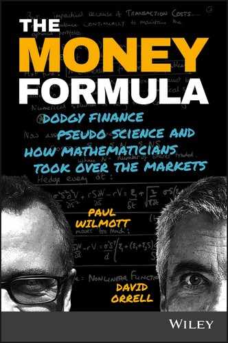
After n iterations, the maximum deviation from 0 is equal to n – so after 14 steps, the range is from −14 to 14. But most paths stay near the center, so the average displacement is much smaller.1 A longer random walk, of 100 steps, is shown by the solid line in Figure 2.3. The light-gray lines are the bounds for possible paths: the upper bound is the path with an increase of 1 at every step, while the lower bound is the path with a decrease of 1 at every step (the probability of these paths is extremely low, since they are the same as tossing a coin and getting heads 100 times in a row). In the background, the density of the grayscale at any point corresponds to the probability of a random walk going through that point. Note how this probability density spreads out with time, rather like an idealized, turbulence-free version of a plume of smoke emitted from a chimney. Random walks sound wild, but on average they are very well-behaved.

Figure 2.3 100-Step random walk
The solid line is a random walk of 100 steps, starting at 0, with a displacement of plus or minus 1 at each step. The light-gray lines show the upper and lower bounds, corresponding to the paths in which the displacement at every step is plus or minus 1, respectively. The density of the grayscale at any point corresponds to the probability of a random walk going through that point. This is highest for paths with small displacement. The probability of a path entering the white area is very low, or zero outside the light-gray lines.
Such computations become unwieldy when there are a very large number of games or iterations; however, in 1738 the mathematician Abraham de Moivre showed that after an infinitely large number of iterations, the results would converge on the so-called normal distribution, or bell curve. This is specified by two numbers: the mean or average and the standard deviation, which is a measure of the curve's width.2 About 68% of the data fall within one standard deviation of the mean, and about 95% are within two standard deviations. The homme moyen of statistics, this formula got its name because of its ubiquity in the physical and social sciences. The distinguishing feature of the normal distribution is that, according to the central limit theorem, which was partially proven by de Moivre, it can be used to model the sum of any random processes, provided that a number of conditions are met. In particular, the separate processes have to be independent of one another, and identically distributed. So, for example, if 18th-century astronomers made many measurements of the position of Saturn in the night sky, then each measurement would be subject to errors, but they could hope that a plot of the measurements would look like a bell curve, with the correct answer close to the middle.
The normal distribution is perhaps the closest the field of statistics comes to a Newtonian formula. The equation is simple and elegant, there are only two parameters that need to be measured (the mean and the standard deviation), and it can be applied to a wide range of phenomena. The “Law of Unreason,” as its Victorian popularizer Francis Galton called it, would find perhaps its greatest application in mastering, or appearing to master, the chaos of the markets.3
Theory of Speculation
The desire to bring order out of chaos, and to see the hidden pattern in the noise, is basic to human nature. In mathematics, even chaos theory is not so much about chaos as about showing that what appears to be wild and unruly behavior can actually be explained by a simple equation. As the field's founder, French mathematician Henri Poincaré, told one of his PhD students: “what is chance for the ignorant is not chance for the scientists. Chance is only the measure of our ignorance.”4
The student who earned this rebuke was called Louis Bachelier. His mistake, perhaps, was choosing a thesis subject that was a little too chaotic – the buying and selling of securities that took place within the mock-Greek temple building of the Paris Exchange, or Bourse. He was awarded a good but undistinguished grade on his 1900 dissertation, entitled Théorie de la Spéculation, and his work failed to unite the academic community in a frenzy of excitement (it took him 27 years to find a permanent job).5
Bachelier began his thesis as follows (imaginary editorial remarks in italics):
The influences which determine the movements of the Stock Exchange are innumerable. Events past, present or even anticipated, often showing no apparent connection with its fluctuations, yet have repercussions on its course. (I had a dog like that once)
Beside fluctuations from, as it were, natural causes, artificial causes are also involved. The Stock Exchange acts upon itself and its current movement is a function not only of earlier fluctuations, but also of the present market position. (Chased its own tail)
The determination of these fluctuations is subject to an infinite number of factors: it is therefore impossible to expect a mathematically exact forecast. Contradictory opinions in regard to these fluctuations are so divided that at the same instant buyers believe the market is rising and sellers that it is falling. (Sounds like we're wasting our time, people)
Undoubtedly, the Theory of Probability will never be applicable to the movements of quoted prices and the dynamics of the Stock Exchange will never be an exact science. (Thought this was a science exam?)
However, it is possible to study mathematically the static state of the market at a given instant, that is to say, to establish the probability law for the price fluctuations that the market admits at this instant. Indeed, while the market does not foresee fluctuations, it considers which of them are more or less probable, and this probability can be evaluated mathematically. (Too much on finance ! – this was a real comment on Bachelier's thesis by France's leading probability theorist, Paul Lévy)
Bachelier's starting assumption, which he called his “Principle of Mathematical Expectation,” was that the mathematical expectation of a speculator is zero. As in the random walks of Figure 2.1, some bets will win, and others will lose, but these cancel out in the long run. Note that we are referring here to the mathematical chances of success – a speculator's psychological expectations may be very different. He then assumed that prices move in a random walk, with price changes following a normal distribution, and referred to what he called the “Law of Radiation (or Diffusion) of Probability,” which described how the future price became more uncertain as you went further into the future. The results are very similar to Figure 2.3 (the displacements at each iteration were there set to plus or minus a fixed amount, in this case 1, rather than being normally distributed, but the effects are almost identical over large enough times). From this, he derived a method for pricing options, which grant the purchaser the right to buy or sell an asset at a fixed price at some time in the future. As discussed further later, the technique he developed is essentially a special case of the ones commonly used today.
To reach his conclusions, Bachelier assumed the existence of a “static state of the market.” This did not mean that prices themselves were static, but that price fluctuations could be modeled as random perturbations to a steady state. The price movements of a stock therefore resembled the so-called Brownian motion of a tiny dust particle, as it is buffeted around by collisions with individual atoms. In 1905, Albert Einstein used techniques similar to those employed by Bachelier to model Brownian motion, and estimate the size of an atom.
Bachelier's thesis eventually became famous in the 1960s, for three separate reasons. The first was empirical, the second was cultural, and the third had to do with a subtle piece of rebranding. The empirical evidence was that price movements did indeed seem to be random, in the sense that no one could accurately predict them. In 1933, a wealthy investor called Alfred Cowles III analyzed the investment decisions of the top 20 insurance companies in the United States and came to the unfortunate conclusion that they showed “no evidence of skill.”6 In 1953, Maurice Kendall found that stock and commodity prices behaved like an “economic Brownian motion,” with random changes outweighing any systematic effects, but was pleased to note that a “symmetrical distribution reared its graceful head undisturbed amid the uproar.”7 And in 1958, the physicist M.F.M. Osborne showed that the proportional changes in a stock's price could be simulated reasonably well by a random walk, as Bachelier had claimed.
The cultural reason for Bachelier's thesis suddenly becoming trendy was that his idea of random walks and probability diffusions fit the post-war scientific zeitgeist. Following the development of quantum theory in the early 20th century, the Newtonian mechanistic model had been replaced with quantum mechanics. In a way this was equally mechanistic (hence the name), but it was now probability waves that were being described mechanistically. According to Heisenberg's uncertainty principle, you could never measure both the exact position and momentum of an object – only the probability that it was in a certain state. Quantum mechanics therefore used probabilistic wave functions to describe the state of matter at the level of the atom. The probability plot of Figure 2.3 above is similar in spirit to the probability plots used to illustrate the behavior of a subatomic particle.
The difference between Newtonian mechanics and quantum mechanics probably seemed rather subtle and abstract to most people, right up until the summer of 1945, when the test detonation of the first atomic bomb in the desert of New Mexico, and the subsequent deployment of the bomb in Hiroshima and Nagasaki, demonstrated both the power, and horror, of the new physics. Research funding poured into weapons laboratories and universities around the world to develop new techniques for analyzing probabilistic systems, and some of this effort spilled over into economics and finance. One example of this research was the Monte Carlo method, which we discuss later. The Black–Scholes equation for option pricing, discussed in Chapter 4, can be rephrased as a probabilistic wave function using the formalism of quantum mechanics.8 Random walk theory was used by physicists to compute the motion of neutrons in fissile material, and therefore the critical mass needed for a nuclear device. Warren Buffett later quipped that “derivatives are financial weapons of mass destruction” (which didn't stop him from being a champion user of them), but their intellectual genesis was largely forged by a real weapon of mass destruction.
Finally, one factor which must have displeased the highly rational examination committee was the fact that Bachelier treated the stock market as being fundamentally irrational. Price changes, he believed, are caused in part by external events, but also represent an internal response, with the market reacting to itself. No one ever has a clear idea what is going on, and opinions about the market “are so divided that at the same instant buyers believe the market is rising and sellers that it is falling.” This jarred with the traditional, mainstream economics view of markets as being inherently rational and self-correcting. Bachelier's theory of speculation therefore became acceptable only when the unpredictability was reframed as being caused not by the market's irrationality, but by its very opposite: incredible efficiency.
All models tell a kind of story about a system. But this was the point where the story became bigger than the model.
Efficient Markets
In another doctoral thesis, published this time by the University of Chicago in 1970, Eugene Fama defined his efficient market as a place where “there are large numbers of rational profit maximizers actively competing, with each trying to predict future market values of individual securities, and where important current information is almost freely available to all participants.”9 In such a market, “competition among the many intelligent participants leads to a situation where, at any point in time, actual prices of individual securities already reflect the effects of information based both on events that have already occurred and on events which as of now the market expects to take place in the future. In other words, in an efficient market at any point in time the actual price of a security will be a good estimate of its intrinsic value.”
Of course, Fama noted, there will always be some disagreement between market participants, but this just causes a small amount of random noise, so prices will wander randomly around their intrinsic values. As soon as prices get too far out of line, the “many intelligent traders” will quickly restore prices to their correct setting.
Fama's view of the market therefore differed from that of Bachelier. The Frenchman had implied that not only was news random, but so was the reaction of investors, with “events, current or expected, often bearing no apparent relation to price variation.” According to Fama, though, an efficient market always reacts in the appropriate way to external shocks; since if this were not the case, then a rational investor would be able to see that the market was over or under-reacting, and profit from the situation. The market's collective wisdom emerged automatically from the actions of rational investors.
Fama's efficient market hypothesis (EMH), which led after 40-odd years to the 2013 economics Nobel, was essentially a more scientific-sounding version of Adam Smith's invisible hand, applied to the stock market. The traditional test of deterministic, scientific models is their ability to use a mechanistic explanation to make accurate predictions. The EMH proposed a specific mechanism – the actions of “rational profit maximizers” interacting in a market – and made a kind of prediction, namely that markets are unpredictable, so no one can consistently beat the market. As Fama argued, this meant that techniques discussed in the next chapter such as chart analysis (looking for recurrent patterns) or fundamental analysis (looking, e.g., for companies that are undervalued relative to earnings or future prospects) can never work, because all the information is immediately priced in by the market. Other forms of quantitative analysis would presumably be equally pointless.
Indeed, empirical evidence does show that markets are hard to predict (different versions of the EMH assume varying amounts of efficiency, and take into account factors such as insider trading, where traders profit from information which is not widely available). The fact that, for example, managed funds find it hard to beat index funds is often deployed as a defense of the EMH.10 As economist John Cochrane wrote, “The surprising result is that, when examined scientifically, trading rules, technical systems, market newsletters, and so on have essentially no power beyond that of luck to forecast stock prices. This is not a theorem, an axiom, a philosophy, or a religion: it is an empirical prediction that could easily have come out the other way, and sometimes does… The main prediction of efficient markets is exactly that price movements should be unpredictable!”11
While the EMH “predicts” that markets are unpredictable, however, one needs to be careful about predictions that only give an explanation for something that is already known. In physics, for example, proponents of string theory have argued that it can predict gravity, but it would be more accurate to say that it offers a possible explanation for something that is already well understood.12 Far more convincing are predictions of things that are not yet known – for example, James Clerk Maxwell's prediction in the 19th century that light is an electromagnetic wave. While the EMH is consistent with markets being unpredictable, you cannot conclude from the unpredictability of markets that they are efficient. In most areas, the fact that something is unpredictable is not interpreted as evidence that it is efficient or hyper-rational. Snow storms are unpredictable, but no one thinks they are efficient. A simpler explanation is that the system is driven by complex dynamics that resist numerical prediction. Many such systems exist – for example, people, clouds, fashions, turbulent flow, the climate, and so on.
Instead, then, it could be that the EMH is right for the wrong reasons. The key assumptions of the theory are that market participants have access to the same information and act in a rational manner to drive prices to an equilibrium. But are these really a sound description of markets?
Irrational Markets
Consider, for example, the idea that investors are rational at least on average. The Greeks said that man was a rational animal, but maybe they were erring on the side of generosity. At the same time that Fama was writing his thesis, the psychologists Daniel Kahneman and Amos Tversky, together with the economist Richard Thaler, were performing psychological experiments that led to the creation of the field known as behavioral economics.13 These experiments demonstrated, rather convincingly, that investment decisions are based on many factors which have little to do with rationality. For example, they showed that we have an asymmetric attitude toward loss and gain: we fear the former more than we value the latter, and bias our decisions toward loss avoidance rather than potential gains. Some of our other various foibles and predilections include the following:
- Status quo bias. We prefer to hold onto things rather than switch to a better alternative – even if it is better. For example, if you inherit $10,000 in Blackberry shares you would be inclined to hold onto them. However, if you were to inherit the same amount in cash you wouldn't put it all into Blackberry.
- The illusion of validity (i.e., denial). We maintain beliefs even if they are at odds with the evidence.
- Loss aversion. We avoid selling poorly performing stocks.
- Power of suggestion. We are influenced by the opinions of others. (We're really enjoying this book so far!) An extreme example is the way traders sometimes egg each other on to take more and more risk.
- Trend following. When the market is going up or down, we think it will continue.
- Illusory correlations. We look for patterns in things like stock prices where they don't exist (they're talking about you, chartists!).
- Immediacy effect. One study showed that we will pay on average 50% more for a dessert at a restaurant when we see it on a dessert cart, rather than when we choose it from a menu.
Many of these behavioral patterns have been confirmed by the experiments of neuroscientists, who put people in scanners and see which parts of their brains light up when offered the choice between a fully funded pension on retirement or an ice-cream that they can have right there! (These profound insights no doubt came as a complete shock to advertisers and retailers, who overnight realized, for the first time in history, that they could continue selling things using sexy images, just like always.)
Of course, one could argue with the neoclassical economists that these peculiarities come out in the wash for a large number of investors. But in a situation like the markets, where investors are influencing and reacting to one another, the opposite is probably true. As Kahneman explains, “when everybody in a group is susceptible to similar biases, groups are inferior to individuals, because groups tend to be more extreme.”14 Indeed, a common phenomenon in markets is herd behavior, where investors rush into, or out of, the same investments together, greatly amplifying risk instead of reducing it. The idea that “many intelligent traders” drive prices to their intrinsic value, so that fluctuations can be considered as random perturbations around an equilibrium state, therefore seems a bit of a stretch. This problem was captured by author James Buchan in his 1997 book Frozen Desire, when he wrote (before the Internet bubble burst): “You buy or sell a security, say the common stock of Netscape Inc., not because you know it will go up or come down or stay the same, but because you want it to do one of those things. What is condensed in a price is the residue not of knowledge but of embattled desire, which may respond to new information and may not. At the time of writing, Netscape is priced in the stock market at 270 years' profits… such a price belongs outside the realms of knowledge. The efficient-markets doctrine is merely another attempt to apply rational laws to an arena that is self-evidently irrational.”15 Or, as Claude Bébéar, founder of the French insurer AXA, put it, mathematical models “are intrinsically incapable of taking major market factors into account, such as psychology, sensitivity, passion, enthusiasm, collective fears, panic, etc. One must understand that finance is not logic.”16
Not Normal
A separate but related question is that of equilibrium. According to Fama, “Tests of market efficiency are tests of some model of market equilibrium and vice versa. The two are joined at the hip.”17 But from the standpoint of complexity science, it makes more sense to view the markets as being, not at some kind of rationally determined equilibrium, but in a state that is far from equilibrium. An early critic of the EMH was Fama's thesis adviser, Benoit Mandelbrot, who pointed out that price changes do not follow a normal distribution, as in the random walk model, but are better modeled by an equally ubiquitous formula known as a power-law distribution, which applies to everything from earthquakes to the size of craters on the moon. For example, the probability of an earthquake varies inversely with size to the power 2, so if you double the size it becomes about 4 times rarer (a number raised to the power 2 is the number squared; a number raised to the power 3 is the number cubed; and so on). In the same way, the distribution of price changes for major international indices have been shown to approximately follow a power-law distribution with a power of about 3.18
The normal distribution is symmetric and has a precise average, which defines a sense of scale. A power-law distribution, in contrast, is asymmetric and scale-free, in the sense that there is no typical or normal representative: there is only the rule that the larger an event is, the less likely it becomes. However, it still allows for extreme events, such as massive earthquakes, or Mississippi Company-style financial meltdowns, which have vanishingly small probability in a normal distribution. The power-law distribution is a signature of systems that are operating at a state that is far from equilibrium, in the sense that a small perturbation can set off a cascade of events (the classic example from complexity research is a finely poised pile of sand, where dropping a single grain might do nothing, or might trigger an avalanche). The normal distribution was derived for cases where processes are random and independent from one another, but markets are made up of highly connected people all reacting to one another. The idea that markets are inherently stable is therefore highly misleading, and as seen in later chapters has led to many problems in quantitative finance.
As a kind of preview, Figure 2.4 is a version of the density plot of Figure 2.3, except that it is based on actual data from the Dow Jones Industrial Index. This index has tracked the performance of 30 large publicly owned companies in the United States since 1928 (earlier versions of the index go back to 1896). The historical time series was divided into sequential segments of 100 days, and we looked at the growth of the index over each 100-day segment.19 If price changes for the companies within the index are “normal,” one would expect the index itself to be too; however, the data swings shown in the plot seem considerably wilder than those of the normal distribution.
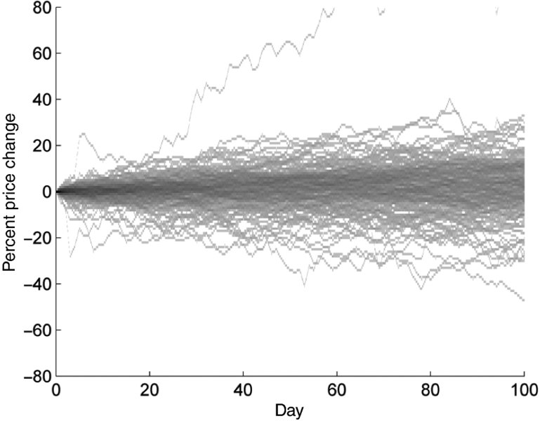
Figure 2.4 Density plot for the Dow Jones Industrial Index, which dates back to Oct 1, 1928
The data was chopped up into segments of 100 days. The growth over each 100-day segment was then plotted, and the results used to calculate a probability density for comparison with previous figures. You can easily distinguish some of the more wild trajectories, which appear as isolated lines.
Figure 2.5 is a histogram of the price changes after 100 days for each segment. Unlike Figure 2.2, the plot is quite asymmetrical and does not seem to approximate a bell curve. The largest increase over a period of 100 days, which occurred during the rebound following the Great Depression, was 79%. Given that the standard deviation of the results is 14.4, the probability of that event, according to the normal distribution, is such that it shouldn't happen once in the age of the universe, let alone the age of the Dow Jones. The reason, of course, is that the data does not follow a normal distribution; if you don't believe in symmetry or efficiency, there is no reason why it should.20

Figure 2.5 Histogram of the price changes after 100 days for each segment of the Dow Jones data
Unlike Figure 2.2, the data does not approximate a bell curve, and there are a significant number of outliers which would be effectively impossible under a normal distribution.
Mental Virus
Given the fact that these flaws in the EMH have been known since the time it was invented, it therefore seems strange that, as noted by The Economist, and explored further in the next chapter, the theory “has been hugely influential in the world of finance, becoming a building block for other theories on subjects from portfolio selection to option pricing.”21
One reason is simply that it enabled both economists and quants to continue using the standard statistical tools they were comfortable with. Power laws may be ubiquitous in nature and finance, but they lack the symmetry, ease of calibration, and mathematical usefulness of the normal distribution. The financial economist Paul Cootner, for example, included a paper by Mandelbrot in his 1964 book The Random Character of Stock Market Prices, but panned him in the introduction by writing that “Mandelbrot, like Prime Minister Churchill before him, promises us not utopia but blood, sweat, toil and tears. If he is right, almost all of our statistical tools are obsolete… Surely, before consigning centuries of work to the ash pile, we should like to have some assurance that all our work is truly useless.”22 (Which is a strange use of Churchill's words, when you think about it – like hearing Churchill say that fighting the Nazis would involve a lot of hard work, so better just to have a good nap.) Mandelbrot's work in finance only became popular in 2007, after more people had become personally acquainted with the idea of a financial earthquake.
Another reason, though, is that as economist Myron Scholes put it, “To say something has failed, you have to have something to replace it, and so far we don't have a new paradigm to replace efficient markets.”23 The traditional test of scientific theories, as mentioned above, is their ability to make predictions. In this case, the main prediction of the theory is that the system is unpredictable. The only way to displace it, by the traditional standard, is to come up with another theory that can make accurate predictions, but that isn't possible. There is no equation, for example, for irrationality (though people have tried). As seen later, hedge funds don't try to predict the global economy, they look for small pockets of predictability in market prices that can be exploited while they last. No one has a perfect model of the economy, and so the theory remains in place. Like some kind of mental virus, it has found a way to disable the usual processes that would get rid of it.
Following the financial crisis, the EMH came under increased scrutiny. To most people, it seemed implausible that markets with such a demonstrated ability to blow themselves up should be described as efficient. In testimony to Congress in 2008, as discussed later, Alan Greenspan did admit that conventional risk theory had failed.24 However, he blamed the problem on only calibrating the models with recent data, and not including periods of historic stress. When asked by The New Yorker in 2010 how the efficient market theory had performed, Fama replied: “I think it did quite well in this episode.”25 The economist Robert Lucas made the usual defense that the reason the crisis was not predicted was because economic theory predicts that such events cannot be predicted.26
This failure to let go of the idea that markets are near-perfect machines is perhaps best explained by behavioral economists – after all, it is typical human behavior to deny there is a problem, cling to the illusion of validity, maintain the status quo, and thus avoid loss. As money manager Jeremy Grantham wrote to his clients in 2009: “In their desire for mathematical order and elegant models, the economic establishment played down the inconveniently large role of bad behavior, career risk management, and flat-out bursts of irrationality… Never underestimate the power of a dominant academic idea to choke off competing ideas, and never underestimate the unwillingness of academics to change their views in the face of evidence. They have decades of their research and their academic standing to defend.”27
Getting academic economists to think identically is like herding sheep. They all go in the same direction, although there's no one with any obvious leadership skills. We will discuss this phenomenon further in Chapter 9. In the next chapters, though, we show how all this theory plays out in the real world (if you consider finance to be the real world). As we'll see, efficiency is a con, and the markets can be gamed. You just need to know the flaws in the system.