“The forecast,” said Mr. Oliver, turning the pages till he found it, “says: Variable winds; fair average temperature; rain at times.”… There was a fecklessness, a lack of symmetry and order in the clouds, as they thinned and thickened. Was it their own law, or no law, they obeyed?

—Virginia Woolf, Between the Acts

“For every expert there is an equal and opposite expert.”

—Arthur C. Clarke

Mathematical models in the real sciences are based on fundamental physical laws and principles. Mass and energy are conserved, to name two obvious examples. But there are no such laws in finance. Financial models are necessarily more qualitative than quantitative. But this doesn't stop the quant thinking he's a scientist. After all, he's more than likely had a scientific education, so it's tempting to think that in going from physics to finance he has merely changed from denim and sneakers to suit and oxfords. He sees an idea like the efficient markets hypothesis and thinks he's back in the quadrangle with Dirac. Sometimes his belief in the models is simple naiveté, sometimes it is physics envy. Either way, it's dangerous to have too much faith in the models. But does the field need less physics – or more?

One great skill in life is to be able to distinguish between problems and opportunities. Going further, surely every motivational speaker tells us that there are opportunities within every problem? “In the middle of difficulty lies opportunity,” said Albert Einstein. He also said, “You think you've got problems. You should see mine!” Large parts of Kipling's If are devoted to precisely this attitude. Miguel de Cervantes said, “As one door shuts another door opens.” Perhaps it was when they were shutting the cell door on him. (Paul's stepfather says, “As one door shuts another door closes,” somewhat less optimistically.) And this is precisely how quantitative finance should be approached.

We've already seen – and we'll discuss it more below – that quantitative finance does not have any of the fundamental building blocks that are throughout the physical sciences, the Newtonian laws for example. Or the perfectly reproducible chemical reactions. In 1991, back when he was chief economist of the World Bank, Larry Summers proclaimed: “Spread the truth – the laws of economics are like the laws of engineering. One set of laws works everywhere.”¹ But there are no “laws of economics.” Nothing is reproducible. They say you can't argue with physics, but you can certainly argue with economics.

Is this a problem?

Hell, no! It's an opportunity!

This is how science works. You see something, perhaps in nature, perhaps in industry, perhaps in finance, that you'd like to understand. You formulate some hypothesis about what's going on. That hypothesis ought to explain what you are seeing, but then so could many theories. Therefore, you seek out new situations that you haven't seen before for which your theory is relevant and see if your hypothesis can predict what happens. If your theory is good at predicting such new results – ideally in as parsimonious a way as possible – then it's a point in favor of your theory. If it's no good then you need to tweak your hypothesis, or maybe even go all the way back to the drawing board. (If your theory is consistent with anything – i.e., it's unfalsifiable – then it's not very useful. See string theory.)

The parsimonious bit is important. You could (well, you couldn't, but you know what we mean) have a giant spreadsheet table listing the gravitational forces between all the bodies in the universe. You could argue that this was a theoretical model of the universe. The table would take the form of a square matrix, with the number of rows and columns being the number of such bodies.²

How does that compare with the simple formula that the gravitational force between two bodies is proportional to the mass of the bodies (m₁ and m₂) and inversely proportional to the square of the distance r between their centers of mass?

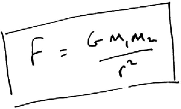
See what we mean by parsimonious? No need for that spreadsheet.

It's important to note that the “laws” have a zone of validity, just like human laws. Hooke's law for springs, for example, says that the force needed to stretch or compress a spring is equal to a constant number multiplied by the extension. Engineers apply it to compute an object's response to a force. However, the formula is a linear approximation which works better for some materials than others – it is not much use for concrete (too brittle), or human tissue (if you pull on your ear lobe, it stretches easily at first but soon becomes very resistant), or rubber (when you blow into a balloon, it is hard at first, then easy, then hard again). Newton's law, meanwhile, is an approximation to Einstein's theory of general relativity, which accounts for the curvature of space-time. According to philosopher Roberto Mangabeira Unger and physicist Lee Smolin, it may be that no laws are completely fundamental and eternal, but themselves evolve with time – as if the universe is learning as it goes.³ For the purposes of modeling, we'll say that a law is a relationship that has been extensively tested and can be treated as fixed and certain within a certain domain.

To summarize, then, the key elements of this process are reproducibility, prediction, and simplicity. Plus knowing where the model breaks down.

• Hooke's law for springs. Applies for materials only within a certain range – and if you stretch anything too far, it will break.
• Newton's law of gravity. Seems to apply everywhere in the visible universe, subject to Einstein's corrections. Unless of course the gravitational force ascribed to “dark matter” is actually due to Newton's law breaking.
• Conservation laws. In his Principia, Newton assumed that, while one substance might conceivably transmute into another (he was an alchemist as well, after all), the total amount of mass in a closed system should remain constant.⁴ Einstein later modified this by showing that energy was another form of mass. Another such principle is conservation of momentum (mass times velocity), which Newton showed was a consequence of his laws of motion.

Even if you're not a mathematician, you can see that these fundamental mathematical models are simple. There's no spreadsheet the size of the universe here. And they just feel right.

A Clue

Quantitative finance does not have any fundamental laws. There's no such thing as conservation, for example. If a share price falls 50% in one day, then half the company's value has just disappeared. If there are no laws, then we might try to rely on statistics. We can still build up a solid model. But if the statistics are not stable, then our model might be limited in accuracy. That's finance.

Consider that old chestnut, the “law of supply and demand.” This states that the market for a particular product has a certain supply, which tends to increase as the price goes up (more suppliers enter the market). There is also a certain demand for the product, which increases as the price goes down. If you plot these two functions – supply and demand – as a function of price, then they form an X pattern, one line going up and the other down, intersecting at a single, correct price. This simple relationship – first illustrated by Scottish engineer (and inventor of the cable car) Fleeming Jenkin in his 1870 essay “On the graphical representation of supply and demand” – does capture a key insight into the way markets work, in a way which has been described as “gratifying and aesthetically pleasing.”⁵ The market value of a product cannot be determined simply by adding up the costs of production and including a profit margin, because if no one wants the product, there won't be a market for it. Conversely, you can't back out all such information just by knowing the market price – something that will be news for many quants who routinely do exactly that for key quantities such as volatility.

But while the supply and demand picture might capture a general fuzzy principle, it is far from being a law. For one thing, there is no such thing as a stable “demand” that we can measure independently – there are only transactions. When a transaction takes place, the buyers and sellers are necessarily in balance (as Bachelier pointed out), and while it may be the case that potential buyers outweigh potential sellers, or vice versa, at any time, this is extremely hard to quantify. Also, the desire for a product is not independent of supply, or other factors, so it isn't possible to think of supply and demand as two separate lines. Part of the attraction of luxury goods – or for that matter more basic things, such as housing – is exactly that their supply is limited. And when their price goes up, they are often perceived as more desirable, not less. This is why the “law of supply and demand” is frequently trotted out to explain why something just happened after-the-fact – as in “this year the price of oil went down because demand decreased” – but is less useful for making accurate predictions (see oil price forecasts). And when someone asserts, for example, that “price is the intersection of two curves, supply and demand,” they are referring to an imaginary thing they have never seen outside their economics textbook.

The “no-arbitrage principle” doesn't quite work either, and for similar reasons. In theory, one should be able to deduce the price of an option from the price and volatility of a stock, on the basis that any departure from that price would create an arbitrage opportunity. But in practice the price of the option is also affected by its own supply and demand, by fear and greed, not to mention all the imperfections such as hedging errors, transaction costs, feedback effects, etc. The role of assumptions such as no arbitrage is again to simply put fuzzy bounds on the relative prices among all the instruments. For example, you cannot have an equity price being 10 and an at-the-money call option being 20 without violating a simple arbitrage. The more realistic the assumption/model, and the harder it is to violate in practice, the more seriously you should treat it. The arbitrage in that example is trivial to exploit and so should be believed. However, in contrast, the theoretical profit you might think could be achieved via dynamic hedging is harder to realize in practice, because delta hedging is not the exact science that one is usually taught. Therefore, results based on delta hedging should be treated less seriously.

However, while there are no fixed laws in financial modeling, there are clues that can point us in the right direction.

Or rather, there's one clue. In the whole of quant finance there is only really one peg onto which we can hang our modeling hat.

The one clue to modeling a share price is… drum roll… we don't care about the share price. (Shurely shome mishtake, ed.)

No, really. We don't care about the price of a share, its numerical value in dollars, pounds, or whatever. No, there's nothing special about $1, or $100, or 10 cents. At least not in absolute terms. Yes, we do care that the share price is now 10 cents since it was $10 when we bought it. But that's a relative thing. The absolute value of the share price doesn't matter, but its value relative to the past does matter.

Think of it this way. If you've got $1000 dollars to invest and the stock is $1, you must buy 1000 shares. If it's $10, you must buy 100 shares. In both cases you have $1000 in stock to start with, and it's how that $1000 changes that you care about. All that you really, really care about is how much the share price has gone up, or gone down, in relative terms. In other words, all that matters is its return. A similar observation inspired Osborne, in his paper on Brownian motion, to note that the model should track proportional price changes (one way to do this is to use a logarithmic scale).

Back to Basics

Why is this an important clue for us modelers? Because it means that in any model we build up we should first study data for the returns, and then model these returns. Suppose, for example, we are trying to model the expected returns of the Dow Jones over a certain time period. Then we could start by plotting some data as we did in Figure 2.5, which showed a histogram of the 100-day returns. One approach would be to use this histogram directly to calculate the probability of a price change within a certain range. Note that even by doing this, we would already be making a couple of critical assumptions. One is that the distribution is stable, so in statistical terms the future will resemble the past. Another is that what happens each period is independent of previous periods, so there is no memory (see also Box 8.1 below).⁶

But it's hard to do any mathematical analysis without equations. So what the mathematician does is to say “Hey, that distribution of returns could be represented by a formula.” And this is where the mathematical modeling comes in, and further assumptions are made.

Some mathematicians will say “It looks like the normal distribution to me, boys!” Which is great, because the normal distribution is easy to work with and has some great properties. Others will say “No, it looks more like [insert favorite (and therefore probably quite complicated) probability distribution here] to me.”

The second group would probably be closer to the truth, since their distribution would be a better fit to the empirical distribution. But their distribution might be so complicated as to limit the usability of the model. The power-law distribution, for example, has no well-defined mean, and is extremely hard to calibrate accurately because the sample of extreme events on which this process depends is by definition small.

In almost all practice it is the normal distribution that is used. So, by a natural process, we end up with a simple random walk of the sort discussed in Chapter 2 (see Figure 2.3). It's the statistical equivalent of fitting a nice straight line to the data. But note how, by choosing the normal distribution, we have already gone from a potentially accurate, albeit unwieldy, model to a toy model.

Even though it's a toy model, it contains a couple of useful ideas that can then be used throughout quantitative finance. These two ideas are just the two parameters in the normal distribution – the average, which tells you the expected return, and the standard deviation, which tells you the volatility.⁷ As we've seen throughout this book, these are very useful, intuitively understandable concepts. But we have to remember their zone of validity. By using the normal distribution, we are saying that extreme events such as Black Monday, or the Flash Crash, or financial crises in general, have effectively zero chance of happening. We are also assuming that the rate of return, and the volatility, will remain constant (recalibration apart).

If these limitations don't trouble us, then as shown in Chapter 3 we could push the idea a little further. Plot risk against reward for a large number of assets. Come up with the idea of a “capital market line,” which draws a straight line through the data, just like Hooke's law. Begin to think of the market as a giant weighing device that stretches returns as you pile on risk.

In derivatives, the volatility is the most important stock parameter. Indeed, we've seen that the expected return doesn't affect the value of an option at all according to the Black–Scholes theory. Volatility is something quite easy to understand, it's how jumpy the stock price is. It's so easy to understand that traders even talk about the value of volatility on the understanding that there's a one-to-one correspondence between the value of volatility and the value of vanilla options. A toy model has led to a good grasp of how options behave, but its variables and parameters – the characters in the story – have also started to take on a life of their own.

A Model for Interest Rates?

Emboldened by having created a toy model that's so-so accurate for stocks, we can ask if perhaps this stock-price model is also good for other financial quantities.

The model we have just built up says that the share-price return is normally distributed with a certain mean and a certain standard deviation. And those two parameters don't depend on the level of the stock. Equivalently, it's like saying that the stock price evolves from one instant to the next with a mean that is proportional to the stock price and a standard deviation proportional to the stock price.

Now, let's see if we can apply similar ideas to modeling interest rates, as a first example of applying the model elsewhere. Can we just replace “share price” in the above with “interest rate”?

Is this a good model: “The interest rate evolves from one instant to the next with a mean proportional to the interest rate and a standard deviation proportional to the interest rate”? Emphatically no! It's instructive to see why.

First of all, stocks tend to keep rising. Not steadily, the volatility makes them bounce around, but in the long run (e.g., Figure 2.5). That's if they survive the long run. Or the company steadily gets worse and the stock falls, and falls. This characteristic is seen in the lognormal random walk model we've built up. If the expected growth is big enough, then the stock will grow over time. If too small, then it will fall. Therefore, if you apply this model to interest rates, they too will either rise indefinitely, or keep falling. Even if the growth rate is set to zero, the expected deviation from its starting point of a random walk could become arbitrarily large. And rates just don't do this in practice. They go up, then come down. They go down, and then rise up. Any model should capture this behavior.

We can do this within the framework we've built up by simply making the expected return and the volatility of interest rates into some function of interest rates. This is easily seen by looking at the expected return. If we make it negative for high interest rates, then high interest rates will tend to fall. If we also make it positive for low rates, then low rates will tend to increase. This is called mean-reverting behavior. In such a model interest rates go up, then fall, then fall, then go back up, just as we see.

But here's our modeling problem. Which function of rates is positive for low values of the rates but negative for high values? Are you kidding? There are an uncountably infinite number of such functions. Which is the right one?

See the problem? In modeling the stock we had to have the expected return function proportional to the stock to get the behavior that the level of the stock didn't matter, only its return. That left one parameter in the expected-return function, the coefficient of proportionality. We have little clue as to what the functional form should be for interest-rate expected growth. And we haven't even started to look at the volatility behavior of rates. Or the question of whether there is a stable value for the mean that we are supposed to be reverting to.

And it's the same problem for anything else we try to model. Credit risk, volatility, etc.

The only half-decent, yet still toy, models in finance are the lognormal random walk models for those instruments whose level we don't care about. That's equities, indices, exchange rates, commodities.⁸ This is why almost everyone is using the lognormal random walk model for these quantities, but there isn't a standard model for interest rates, everyone uses something different. There's no bollard on which to moor our interest-rate modeling boat. But that doesn't mean we can't make some progress. For inspiration, we can turn to an area with a different history and set of approaches – mathematical biology.

A Role Model

In the mid-1980s one of the hottest mathematical topics was that of mathematical biology. There's no better way to describe this subject than to skim through the contents of possibly the best book on mathematical modeling (and not just in biology) ever written, Mathematical Biology by Jim Murray. The edition to which we'll refer is the first, published in 1989. To date this is the only mathematics book that Paul has ever read in bed. We would recommend this book to anyone doing modeling in any field whatsoever – even, or perhaps especially, quant finance. It is highly inspirational, and also covers many different mathematical fields.

The first four chapters are about population dynamics. For example, modeling how the population of the spruce budworm changes due to births and deaths. The resulting model shows how the population can have one or three steady states, depending on parameters in the model. (One is tempted to think of interest rates as a financial quantity that might also exhibit steady states, states that change depending on parameters such as official policy.) We are up to page 7 of Professor Murray's book. From page 8 we learn about delay models. In practice, there is a delay between the birth of a budworm and it reaching maturity and in turn reproducing. (Hmm… a change in interest-rate policy might be flagged by the policy makers but with a delay before implementation. It's not different to see parallels between mathematical biology models and finance.) The delay models are also relevant in some diseases, for example Cheyne–Stokes respiration (we are on page 15). This is not related to populations, but the delay is due to a time lag between a change in the level of carbon dioxide in the blood and its observation in the brain. (Time lag? Observation? “News”! Makes us think of everything financial, after all, it's news which drives much of the change in market prices. And today there are several vendors selling data feeds of news, search terms on Google, and twitter trends precisely so people, or their text-reading algorithms, can get one step ahead of the news.)

Page 29 introduces us to age distribution. People are born, get older, die. Can we figure out the number of people at any age? Yes. Not deterministically perhaps, but probabilistically yes. This is a subject well covered by actuarial science.¹⁰ On page 41 of Chapter 2 we are shown how a simple population model, first developed by ecologist Robert May, leads to the nonlinear logistic model and chaos. In Chapter 3 we have interacting populations, for example the classical lion–gazelle-type models. The lions eat the gazelles, causing the gazelle population to fall. The lions have nothing to eat, their population falls. This allows the gazelle population to build up. As does the lion population in response. (Now, if that isn't a toy model of how interest rates and inflation dance around we don't know what is.) Such models help in the management and conservation of species, helping to determine, for example, whether culling is beneficial.

Seventeen more chapters to go (including appendices and index, the book is 696 pages long). Reaction kinetics, coupled oscillations, chemotaxis, animal coat patterns, epidemics, etc. But we've made our point. There is a richness in mathematical biology, in the subjects addressed and the mathematics used, that ought to be seen in mathematical finance.

The above are almost all toy models. None can predict with pinpoint accuracy the dynamics of the bumble-bee population, and they can't tell you exactly how many spots there will be on a leopard. But all can be used to explain what is seen in nature, and all can be used to help in the control of species where necessary, to aid in the development of pesticides, to fight against disease, or to aid conservation, etc.

Many of the modeling ideas could be used to advantage in finance, economics, government policy making, etc., which seem relatively stuck in the past. As Robert May told the Financial Times, “The more I hear about financial economics, the more I am struck by its similarity to ecology in the 1960s.”¹¹ But we bet there are more mathematical biologists wanting to learn the relatively straightforward subject of quant finance than there are quants wanting to learn the tools of mathematical biology. Incidentally, Jim shows how a random walk leads to the diffusion equation, the mainstay of quant finance, in pages 232 to 236. That's five pages. Finance authors can take an entire book to do this simple job.

Is mathematical biology still a science? Sure. You don't need perfect models to be a science – otherwise hardly anything would qualify. Biological models might simplify very complicated processes, and be qualitative rather than purely quantitative, but they still give useful insights into mechanisms and behaviors.

Why are these toy models? In very few of the models in Jim Murray's book are there any reliable physical laws. The main exception being those based on chemistry. In Section 15.2 we see a model for pattern formation in butterfly wings based on the diffusion of morphogens through the wing. Now, the diffusion equation can be very accurate but given that the wing coloration is happening at a cellular level, and with the complex geometry of the wing and the veins, we cannot expect the model to give anything other than the gross features of the pattern.

In just this one field of mathematical biology we see a great variety of mathematics. And it is precisely because there are no fundamental laws that researchers have the freedom to use whatever mathematics they fancy. And that is what makes mathematical biology as a research field such a joy – the total, uninhibited freedom one has to model in whatever way works.

In the decades since Murray wrote his book, the techniques used in computational biology have expanded to include things such as network theory, complexity theory, and the machine learning techniques discussed in Chapter 6, which are ideally suited for analyzing and searching for patterns in large quantities of data, such as genomes. Now, we aren't saying that we should be transferring technology en masse from mathematical biology to quantitative finance. No, that would be silly. Yes, we, seasoned mathematical modelers that we are, can find parallels between things in biology and things in finance literally as fast as we are typing, but that was just an intellectual exercise. We are saying that quantitative finance could benefit from being approached in a similar manner.

Embrace the fact that the models are toy, and learn to work within any limitations. Focus more attention on measuring and managing resulting model risk, and less time on complicated new products.

In fact, the same could be said of life in general. We all carry our mental models of reality around in our head. We all try to shoehorn experience into our preconceived structures. But only by remaining both skeptical and agile can we learn. Keep your models simple, but remember they are just things you made up, and be ready to update them as new information comes in.

Reasons to be Mathematical

If all finance models are inevitably toys, then why do abstract fields such as measure theory (which generalizes measures such as length or area and is used in advanced probability theory) have such a stranglehold on the subject? Why go to such lengths to rigorously prove over and over again what is quite frankly obvious to any seasoned mathematician? Why is the subject so insistent about maintaining the appearance of mathematical exactness? There are a number of reasons:

• Envy. Mathematical biologists are comfortable working with toy models. They tend to be people from a solid mathematics background and know their strengths and weaknesses. They are quite at ease with themselves. In contrast, most people working in quantitative finance come from finance or economics or computer science. And quant finance is their big break, they can now proudly tell their parents that they are proper mathematicians. But only if they can fool people that the mathematics is hard enough. Measure theory can be very hard. It's quite abstract. But it's also something that is seen in the first year of an undergraduate mathematics degree. However, being abstract gives it a kudos that more practical mathematics, applied mathematics, doesn't have. It's like the Emperor's new clothes. Okay, we'll be the little boy in the story: “Look, Mummy, they're only doing first-year math!”

• Education. Masters programs in mathematical finance have almost all been made in the same image. We can see the scenario 20 years ago at a meeting of the mathematics faculty at one of the less prestigious universities. The chairman gets to the part in the agenda were they are to discuss a new degree program in mathematical finance. The chairman asks the faculty members if they know anything about the subject in question. None do. Okay then. “Anyone know measure theory?” A few shy hands go up. “Then let's rebrand the measure theory courses as mathematical finance. Let's rock'n'roll!” Except the chairman wouldn't say “Let's rock'n'roll.”

• Inertia. Inertia is the wrong word for this. But what we mean is that there's no incentive to incorporate more or better mathematical models into this business. There is so much money in derivatives and banking generally that all you need to make a ton of money is to not get into any trouble and just cream your percentage off the top.

• Credibility. At the same time, the fact that there are massive amounts of money at stake is scary and means that you want your model to be based on something that is solid, or at least conforms to agreed standards. You also want to be able to talk in a convincing way about risk analysis. The expression “toy model” is unlikely to play well. In this respect, finance is more like engineering. But engineers rely on well-tested results such as Hooke's law to make their calculations; they know to build in a margin of error, and they are keenly aware of where their models break down.
• Consistency. Finally, a related reason why finance has evolved the way it has is that the subject's mental DNA – to employ a biological metaphor – is based on fixed ideas, imported from economic theory, about the way the world works. While economics does not have conservation laws, it does have its economic principles. These include the ideas that investors have similar power and access to information; that they act rationally and independently to optimize their own utility; and that as a result, markets are drawn to a stable equilibrium. The advantage of these highly restrictive assumptions is that they allow economists to develop theoretical models which link the micro level of the economy (e.g., the behavior of individual investors) to the macro level (e.g., market statistics). Instead of a collection of modeling techniques developed for special cases, as in computational biology, the result is a single, consistent, and above all authoritative story.

The problem is that, in the quant's mind, the effect of all this intellectual baggage is that the toy model looks like a real model based on sound principles. He begins to believe that “one set of laws works everywhere.” As a result, the toy model gets used outside its zone of validity. An example is the assumption that market returns follow a normal distribution, when in fact empirical evidence shows that they don't, not really. Models based on such idealized assumptions are useful within a certain context, but – like the software packages used in engineering – should carry warning labels to the effect that they are hazardous if applied inappropriately.

These restrictive assumptions have never been adopted in computational biology or ecology, for the obvious reason that they don't work. Ecosystems are non-homogeneous and asymmetric, which is what drives changes and diversity. (In an economist's version of a jungle, all the animals would be white mice.) And in biology, the only systems that are stable are dead.

Quantum Finance

In any case, while it is often said that finance models itself after physics, it is more accurate to say that it has modeled itself after Newtonian physics, which is not quite the same thing, being a little out of date. At the start of the 20th century, physics was shaken to its roots by the quantum revolution. This showed that matter is not made up of billiard-ball particles bouncing off one another, but instead is fundamentally dualistic. Subatomic entities such as electrons behave in some ways like particles, and in other ways like waves.

One implication was that it was impossible to make accurate measurements for subatomic systems. The Heisenberg uncertainty principle, which stated that we can't know both the momentum and the location of a particle to complete accuracy, seemed to say that we could make no precise predictions. However, quantum mechanics did allow physicists to make probabilistic statements which specified the chance of an event, such as the probability of an atom of uranium emitting a particle of alpha radiation (useful in designing atomic bombs).

At the same time, though, it was found that the quantum nature of particles added a rich layer of complexity to atomic interactions, giving them, we could say, a life of their own. As a result, we can't divine much about a material's properties by analyzing its components. An example is water: when it freezes, it expands instead of contracting, which means that ice floats on water rather than sinking to the bottom (useful for life in lakes). But that remarkable property can't be predicted or modeled from a knowledge of water's atomic structure, because it depends on the amazingly complex interactions between water molecules.¹² It is better described as an emergent property of the system.

In finance there is a similar situation. Consider, for example, the nature of money. Standard economic definitions of money concentrate on its roles as a “medium of exchange,” a “store of value,” and a “unit of account.” Economists such as Paul Samuelson have focused in particular on the first, defining money as “anything that serves as a commonly accepted medium of exchange.” This definition is similar to John Law's definition of money as a “Sign of Transmission.” Money is therefore not something important in itself; it is only a kind of token. The overall picture is of the economy as a giant barter system, with money acting as an inert facilitator.

However, as David has argued at great and some would say inordinate length elsewhere, money is far more interesting than that, and actually harbors its own kind of lively, dualistic properties.¹³ In particular, it merges two things, number and value, which have very different properties: number lives in the abstract, virtual world of mathematics, while valued objects live in the real world. The tension between these contradictory aspects is what gives money its powerful and paradoxical qualities. A money object such as a dollar bill is a physical object that can be traded, valued, and possessed, but unlike other things in the economy it has a fixed, numerical price. Prices for other things emerge from the use of these money objects – just as the properties of water emerge from interactions between molecules.

Of course, something like an electronic transfer, or a bitcoin, does not resemble the Newtonian idea of a self-contained object – but then neither does matter when viewed from a quantum perspective. The real and the virtual become blurred, in physics or in finance. And just as Newtonian theories break down in physics, so our Newtonian approach to money breaks down in economics. In particular, one consequence is that we have tended to take debt less seriously than we should (more on this in Chapter 10).

Now, in the 1950s, when quantitative finance was in its infancy, the fact that things had moved on in physics was not a problem – it was an opportunity! Unfortunately, quants didn't take it. Or rather, they took the wrong one. Instead of facing up to the intrinsically uncertain nature of money and the economy, relaxing some of those tidy assumptions, accepting that markets have emergent properties that resist reduction to simple laws, and building a new and more realistic theory of economics, quants instead glommed on to the idea that, when a system is unpredictable, you can just switch to making probabilistic predictions. The efficient market hypothesis, for example, was based on the mechanical analogy that markets are stable and perturbed randomly by the actions of atomistic individuals. This led to probabilistic risk-analysis tools such as VaR. However, in reality, the “atoms” are not independent, but are closely linked, like the molecules in water. The result is the non-equilibrium behavior, such as sudden phase changes and turbulence, observed in real markets. Markets are unpredictable not because they are efficient, but because of a financial version of the uncertainty principle.

As discussed in Chapter 2, the great advantage of probabilistic predictions is that they sound authoritative, but are hard to prove wrong because to do so takes a great deal of data. If you say there is only a 5% chance of a market crash, and there is indeed a crash, then you can just say it was bad luck. Theories are almost impossible to falsify. Finance therefore took exactly the wrong lesson from the quantum revolution. It held on to its Newtonian, mechanistic, symmetric picture of an intrinsically stable economy guided to equilibrium by Adam Smith's invisible hand. But it adopted the probabilistic mathematics of stochastic calculus. The result was that, instead of a financial version of E = mc², we got an uncontrolled global credit bomb.

Order and Chaos

To summarize, markets are not determined by fundamental laws, deterministic or probabilistic. Instead, they are the emergent result of complex transactions. They constitute a living system, not a dead one. While it is often said that the economy is ruled by fixed laws – one sample headline reads: “China learns it can't control the laws of economics” – it would be more accurate to refer to the wildness of the economy. This changes the way that we see financial modeling. In particular, money should play a central role, similar to that of a biologically active substance.

One of the more obvious properties of money is that it has a profound effect on human psychology. Neuroscientist Brian Knutson, who investigated this in a series of experiments, said that “Nothing had an effect on people like money – not naked bodies, not corpses. It got people riled up. Like food provides motivation for dogs, money provides it for people.”¹⁴ (Observe quant behavior just before feeding bonus time.) It therefore seems bizarre that economics and finance, since the time of Adam Smith, have treated money as nothing more than an inert medium of exchange. For example, the models used by policy makers usually don't even include a banking or finance sector – which makes banking crises rather hard to predict.¹⁵ But only by omitting money could theorists maintain the pretense that the economy was an orderly, rational, efficient system.

Of course, merely strapping a financial sector onto traditional models will not necessarily make them more predictive or useful. The more apparently realistic you make a model, the less useful it often becomes, and the complexity of the equations turns the model into a black box. The key then is to keep with simple models, but make sure that the model is capturing the key dynamics of the system, and only use it within its zone of validity. Models should be seen as imperfect patches, rather than as accurate representations of the complete system. Instead of attempting to replace traditional theory with a better, more complete “theory of everything,” the aim is to find models that are useful for a particular purpose, and know when they break down.

Another approach is to go the Renaissance route, abandon the idea of mechanistic modeling, and just let the computer look for patterns in data. The resulting models may be more parsimonious than a fully mechanistic model, but are a black box in the sense that the equations do not typically correspond to easily understood mechanisms. They therefore lack some of the advantages of simple mechanistic models, such as the ability to test hypotheses, or make qualitative predictions for situations where prior data is not available. However, they are better suited than mechanistic models for handling the massive amounts of financial and other data which have become available in recent years.

Perhaps the best approach is to use a mix of techniques, while being aware of the advantages and disadvantages of each. The worst is to pretend that toy models are actually fundamental laws of the universe – and then bet a quadrillion dollars on them. So this is where abstract ideas about models have very real implications. If you think models are just useful approximations to the far more complex reality, you tend to be more careful about using them.

As discussed earlier, one of the main motivations in financial modeling, apart from pay, has been aesthetics. We are attracted by the beauty of our models, and come to think that they are true. The move from a Newtonian, mechanistic approach to a complexity approach can therefore be viewed in terms of an aesthetic shift. Instead of independent atom-like investors, we have connected networks. Instead of static equilibrium, we have dynamic motion. And instead of linearity and symmetry, we have nonlinearity and asymmetry.

So now that we have shown some alternative, if more humble and limited approaches to financial modeling, will the banks and universities be racing to update their models? Certainly not – because whether dealing with investors, regulators, or the public, or even just for making money, accuracy isn't really the point. What counts is the impression of accuracy, which is much better served by a model in which the economy is at equilibrium, and risk can be precisely calculated, than one in which the economy is far from equilibrium and risk is essentially unquantifiable. This will become clearer in the next chapter, where we turn to another kind of asymmetry – the balance, or lack thereof, between risk and reward – and how quants have learned to exploit it at the expense of investors.