Chapter 1
Redundancy Resolution via Pseudoinverse and ZD Models
1.1 Introduction
Recently, robotics has played a more and more important role in scientific research and engineering applications [1–4]. Being an essential topic, the problem of redundancy resolution (or mostly say, the problem of inverse kinematics, which is related to the kinematic control of some redundant robot manipulator) has attracted the extensive attention of many researchers [5–9]. The general description of such a problem is that, given the desired Cartesian path ![]() of the end-effector versus time
of the end-effector versus time ![]() , the corresponding trajectories of joint-variable vector
, the corresponding trajectories of joint-variable vector ![]() need to be obtained online (or offline and in advance). In mathematics, to find
need to be obtained online (or offline and in advance). In mathematics, to find ![]() such that
such that
where forward-kinematics mapping ![]() is nonlinear and differentiable with a known structure and parameters for a given robot manipulator [1–3, 9]. Note that, for a redundant robot manipulator, it possesses more degrees of freedom (DOF) than necessary to perform a user-specified end-effector primary task (in mathematics,
is nonlinear and differentiable with a known structure and parameters for a given robot manipulator [1–3, 9]. Note that, for a redundant robot manipulator, it possesses more degrees of freedom (DOF) than necessary to perform a user-specified end-effector primary task (in mathematics, ![]() ) [1–3]. The extra DOF allow the existence of an infinite number of feasible solutions to the redundancy-resolution problem. This can be utilized to determine the best joint-variable, joint-velocity, and/or joint-acceleration vectors in some sense (for a specified end-effector pose, velocity, or acceleration vector), which corresponds to an optimality criterion [9]. Thus, many studies have reported on the kinematic control of redundant robot manipulators [5–11].
) [1–3]. The extra DOF allow the existence of an infinite number of feasible solutions to the redundancy-resolution problem. This can be utilized to determine the best joint-variable, joint-velocity, and/or joint-acceleration vectors in some sense (for a specified end-effector pose, velocity, or acceleration vector), which corresponds to an optimality criterion [9]. Thus, many studies have reported on the kinematic control of redundant robot manipulators [5–11].
The pseudoinverse-based approach represents the conventional solution to the redundancy-resolution problem, which can be analytical. In general, it contains one minimum-norm particular solution plus a homogeneous solution. This simple characteristic has made the research and application of such a pseudoinverse-based approach popular in recent decades [3, 5–7, 9–11]. For example, in [7], a multi-objective approach is investigated for the motion planning of redundant robot manipulators, which combines the closed-loop pseudoinverse method and a multi-objective genetic algorithm. Among the pseudoinverse-based techniques for robotic redundancy resolution, the minimum velocity norm (MVN) scheme, which aims at minimizing the sum of squares of joint velocities, has been widely adopted by researchers for the kinematic control of redundant robot manipulators [1–3, 9]. In addition, to guarantee the high precision of the end-effector positioning (i.e., the small or tiny position error of the end-effector), the corresponding feedback can be added to such a pseudoinverse-based MVN scheme. Thus, with time argument ![]() omitted here (and sometimes afterward) for presentation convenience, the pseudoinverse-based MVN scheme with feedback (being a closed-loop scheme) is formulated as
omitted here (and sometimes afterward) for presentation convenience, the pseudoinverse-based MVN scheme with feedback (being a closed-loop scheme) is formulated as
where ![]() is the joint-velocity vector;
is the joint-velocity vector; ![]() denotes the pseudoinverse of the Jacobian matrix
denotes the pseudoinverse of the Jacobian matrix ![]() ; and
; and ![]() is the desired Cartesian velocity vector, that is, the time-derivative vector of the desired end-effector path
is the desired Cartesian velocity vector, that is, the time-derivative vector of the desired end-effector path ![]() . Besides,
. Besides, ![]() is the feedback gain of position error
is the feedback gain of position error ![]() . Note that pseudoinverse-based MVN scheme (1.1) can actually be obtained by defining the aforementioned error function
. Note that pseudoinverse-based MVN scheme (1.1) can actually be obtained by defining the aforementioned error function ![]() and exploiting the neural-dynamics method presented in [12, 13] (i.e., the method of zeroing dynamics, ZD, presented in this chapter as well). Compared with the widely-used constraint (i.e.,
and exploiting the neural-dynamics method presented in [12, 13] (i.e., the method of zeroing dynamics, ZD, presented in this chapter as well). Compared with the widely-used constraint (i.e., ![]() ) in the existing literature [1, 2, 9], a prominent advantage of the feedback-added constraint is that it guarantees the error
) in the existing literature [1, 2, 9], a prominent advantage of the feedback-added constraint is that it guarantees the error ![]() with no drifting/diverging happened. This also means that the error drift/divergence phenomenon in pseudoinverse-based MVN scheme (1.1) does not exist. Besides, one of the main reasons for the popularity of the two-norm as an optimality criterion is the fact that the related optimization problems yield closed-form analytical expressions. Thus, in many robotic applications, the two-norm optimality criterion is utilized, more because of its mathematical tractability than physical desirability [9]. On the basis of these considerations, pseudoinverse-based MVN scheme (1.1) for redundant-manipulator kinematic control is the focus of this chapter.
with no drifting/diverging happened. This also means that the error drift/divergence phenomenon in pseudoinverse-based MVN scheme (1.1) does not exist. Besides, one of the main reasons for the popularity of the two-norm as an optimality criterion is the fact that the related optimization problems yield closed-form analytical expressions. Thus, in many robotic applications, the two-norm optimality criterion is utilized, more because of its mathematical tractability than physical desirability [9]. On the basis of these considerations, pseudoinverse-based MVN scheme (1.1) for redundant-manipulator kinematic control is the focus of this chapter.
In recent years, as a branch of artificial intelligence, artificial neural networks (ANNs) have attracted considerable attention as candidates for novel computational systems [1, 2, 12, 13]. Being a special type of ANNs, recurrent neural networks (RNNs), which originate from the research of Hopfield neural network [14], have been developed and investigated for solving a wide variety of mathematical problems arising in numerous fields of science and engineering [1, 2, 12]. Note that, compared with conventional numerical algorithms, the dynamics approach based on RNNs has several potential advantages in real-time applications, for example, high-speed parallel-processing, distributed-storage, and adaptive self-learning natures. Therefore, such an approach is generally taken into account as a powerful alternative to online computation and optimization. Especially for robotic redundancy resolution, various RNN models have been developed, exploited, and investigated [1, 2, 15–17].
As for pseudoinverse-based MVN scheme (1.1), the problem of time-varying matrix pseudoinversion is involved in the scheme formulation. It is worth pointing out here that, owing to its fundamental roles, much effort has been devoted to the fast solution of matrix pseudoinversion problem, and many models have been presented by researchers [18–22]. However, the investigations and revisit on those models are not the emphases in this book and thus will not be covered.
Gradient dynamics (GD) and zeroing dynamics (ZD) are two powerful dynamics approaches based on RNNs, which are regarded as two alternatives for online computation, and have widely arisen in scientific and engineering fields, drawing extensive interests and investigation of researchers [18, 23]. In particular especially, GD models are proposed and investigated in [18], which use the Frobenius norm of the error matrix as the performance criterion and evolve along the negative gradient-descent direction to make the error norm decrease to zero with time in the time-invariant case. Recent researches have shown that such a GD approach can also be developed and generalized for time-varying problems solving [12, 13]. Besides, the ZD approach, which is based on an indefinite matrix/vector-valued error function, has been presented for time-varying problems solving, such as the time-varying matrix pseudoinversion [12, 23]. It is worth providing the conceptions of ZD and GD here to lay a basis for further investigation.
Compared with GD, the ZD design is based on a matrix-valued indefinite error function and an exponent-type formula (i.e., the ZD design formula), which makes every element of the error function exponentially converge to zero. By making good use of the time-derivative information of the time-varying coefficient, the resultant ZD models can effectively avoid the lagging errors and can exponentially converge to the theoretical pseudoinverse of time-varying matrix (e.g., the Jacobian matrix ![]() involved in this chapter) [23].
involved in this chapter) [23].
On the basis of the successful work [12, 23, 24], this chapter presents and investigates the application of discrete-time ZD models to kinematic control of redundant robot manipulators via time-varying Jacobian matrix pseudoinversion. That is, by computing the time-varying pseudoinverse of the Jacobian matrix, the resultant ZD models are applied to redundant-manipulator kinematic control. Simulation results based on a five-link robot manipulator and a three-link robot manipulator are illustrated to show the effectiveness of the presented ZD models for time-varying matrix pseudoinversion applied to the redundancy resolution of robot manipulators.
1.2 Problem Formulation and ZD Models
In this section, based on the previous work [12, 23, 24], the discrete-time ZD models are presented and investigated for time-varying Jacobian matrix pseudoinversion.
1.2.1 Problem Formulation
In order to lay a basis for further investigation, the preliminaries and problem formulation of time-varying matrix pseudoinversion are presented next.
Note that the time-varying Jacobian pseudoinverse ![]() always exists and is unique [25]. In this chapter, we only consider the situation of
always exists and is unique [25]. In this chapter, we only consider the situation of ![]() . In particular, if Jacobian matrix
. In particular, if Jacobian matrix ![]() is of full rank at any time instant
is of full rank at any time instant ![]() , that is,
, that is, ![]() , we have the following lemma about the time-varying pseudoinverse of
, we have the following lemma about the time-varying pseudoinverse of ![]() .
.
As the time-varying pseudoinverse ![]() satisfies the corresponding matrix equation
satisfies the corresponding matrix equation ![]() , the following problem formulation of continuous-time varying Jacobian matrix pseudoinversion can be considered and/or checked for the solution correctness:
, the following problem formulation of continuous-time varying Jacobian matrix pseudoinversion can be considered and/or checked for the solution correctness:
where ![]() is the time-varying unknown matrix to be obtained. To lay a basis for further discussion,
is the time-varying unknown matrix to be obtained. To lay a basis for further discussion, ![]() is assumed to be of full rank at any time instant
is assumed to be of full rank at any time instant ![]() . In other words, the configuration singularity for the redundant robot manipulator does not exist during the motion-task execution.
. In other words, the configuration singularity for the redundant robot manipulator does not exist during the motion-task execution.
1.2.2 Continuous-Time ZD Model
To design and control the solving process of the problem (1.3), the following matrix-valued indefinite error function is defined:
Then, based on the ZD design methodology [12], specifically, ZD design formula ![]() with
with ![]() , we can obtain
, we can obtain ![]() . From
. From ![]() , with
, with ![]() being the identity matrix, we have an underdetermined system:
being the identity matrix, we have an underdetermined system: ![]() , of which the minimum norm solution is
, of which the minimum norm solution is ![]() . Thus, we have the following dynamic equation:
. Thus, we have the following dynamic equation:
From (1.5), postmultiplying ![]() and knowing
and knowing ![]() , we have
, we have
Evidently, Equation (1.6) is underdetermined and for this the minimum norm solution exists. That is, we have the minimum norm solution to it:
which is termed the continuous-time ZD model. Note that continuous-time ZD model (1.7) is also the Getz–Marsden (G-M) dynamic system for time-varying pseudoinversion [23].
1.2.3 Discrete-Time ZD Models
For the purposes of possible hardware implementation, for example, the digital computer or the digital circuit, the discrete-time ZD (DTZD) models are presented and developed in this section for time-varying pseudoinversion (1.3).
1.2.3.1 Euler-Type DTZD Model with  Known
Known
In order to discretize the presented continuous-time ZD model (1.7) for solving time-varying pseudoinverse, we refer to the following Euler forward-difference rule [26, 27, 29]:
where ![]() denotes the sampling period, and update index
denotes the sampling period, and update index ![]() . In general, we denote
. In general, we denote ![]() for presentation convenience. In addition,
for presentation convenience. In addition, ![]() and
and ![]() (which is assumed to be known) are discretized by the standard sampling method, of which the sampling period is also
(which is assumed to be known) are discretized by the standard sampling method, of which the sampling period is also ![]() . For convenience and also for consistency with
. For convenience and also for consistency with ![]() , we use
, we use ![]() standing for
standing for ![]() and
and ![]() standing for
standing for ![]() . Thus, we discretize continuous-time ZD model (1.7) as
. Thus, we discretize continuous-time ZD model (1.7) as
where step-size ![]() . For presentation convenience, in this chapter, the discrete-time model (1.9) is called the Euler-type DTZD model with
. For presentation convenience, in this chapter, the discrete-time model (1.9) is called the Euler-type DTZD model with ![]() known, that is, the EDTZD-K model.
known, that is, the EDTZD-K model.
1.2.3.2 Euler-Type DTZD Model with  Unknown
As probably we know, in real-world applications, the analytical form or numerical value of ![]() may be difficult to know. Thus, it is worth investigating the discrete-time ZD model when
may be difficult to know. Thus, it is worth investigating the discrete-time ZD model when ![]() is unknown. In this situation,
is unknown. In this situation, ![]() is generally estimated from the existing data of
is generally estimated from the existing data of ![]() by employing the following Euler backward-difference rule [27]:
by employing the following Euler backward-difference rule [27]:
where ![]() is defined the same as before. Similarly, we define
is defined the same as before. Similarly, we define ![]() and
and ![]() for presentation convenience. From EDTZD-K model (1.9), we derive the Euler-type DTZD model with
for presentation convenience. From EDTZD-K model (1.9), we derive the Euler-type DTZD model with ![]() unknown (i.e., EDTZD-U model) for time-varying pseudoinversion as follows:
unknown (i.e., EDTZD-U model) for time-varying pseudoinversion as follows:
Note that, from the Euler backward-difference rule, we can not estimate ![]() since
since ![]() starts from 0 s and
starts from 0 s and ![]() is undefined. In this situation, we choose
is undefined. In this situation, we choose ![]() (i.e.,
(i.e., ![]() ) to start the update (1.10). That is, at the first update, the EDTZD-U model is
) to start the update (1.10). That is, at the first update, the EDTZD-U model is
which initiates the iterative computation of EDTZD-U model (1.10).
1.2.3.3 Taylor-Type DTZD Models
In order to achieve a higher computational accuracy in the ZD discretization for solving time-varying pseudoinverse, we refer to the following Taylor forward-difference rule [26]:
Thus, we discretize continuous-time ZD model (1.7) as
For presentation convenience, Equation (1.12) is called the Taylor-type discrete-time ZD model with ![]() known, that is, the TDTZD-K model.
known, that is, the TDTZD-K model.
As we know, it may be difficult to know or obtain the value of ![]() directly in certain real-world applications. In this situation,
directly in certain real-world applications. In this situation, ![]() can be estimated from
can be estimated from ![]() by employing the backward-difference rule of the first-order derivative with a third-order accuracy [27]:
by employing the backward-difference rule of the first-order derivative with a third-order accuracy [27]:
Thus, the Taylor-type discrete-time ZD model with ![]() unknown (i.e., the TDTZD-U model) can be formulated as
unknown (i.e., the TDTZD-U model) can be formulated as

The classical Newton iteration is generalized and developed to solve (1.3), which is formulated as [28]:
It is noted that three initial states ![]() ,
, ![]() and
and ![]() are needed for the initialization of TDTZD-U model (1.14). Besides, from (1.13), we can not obtain
are needed for the initialization of TDTZD-U model (1.14). Besides, from (1.13), we can not obtain ![]() since
since ![]() starts from 0 s and thus
starts from 0 s and thus ![]() is undefined. Thus, in the ensuing applications to the redundancy resolution of robot manipulators, in view of the fact that the Newton iteration has the simplest structure, we exploit Newton iteration (1.15) for the initializations of the TDTZD-K (1.12) and TDTZD-U models (1.14).
is undefined. Thus, in the ensuing applications to the redundancy resolution of robot manipulators, in view of the fact that the Newton iteration has the simplest structure, we exploit Newton iteration (1.15) for the initializations of the TDTZD-K (1.12) and TDTZD-U models (1.14).
1.3 ZD Applications to Different-Type Robot Manipulators
In this section, based on a five-link planar robot manipulator and a three-link planar robot manipulator, computer simulations are conducted to illustrate the effectiveness of the presented discrete-time ZD models for redundant-manipulator kinematic control.
For a better understanding, the block diagram of the kinematic-control system that incorporates pseudoinverse-based MVN scheme (1.1) and the presented ZD models is illustrated in Figure 1.1.
1.3.1 Application to a Five-Link Planar Robot Manipulator
In this subsection, the presented discrete-time ZD models and Newton iteration are applied to the kinematic control of a five-link planar robot manipulator with its geometry illustrated in Figure 1.2. For such a robot manipulator, each element of Jacobian matrix ![]() is presented as follows:
is presented as follows:

where ![]() (with
(with ![]() ) denotes the length of the
) denotes the length of the ![]() th link. In addition,
th link. In addition, ![]() and
and ![]() . For simplicity and illustration, with each link length being 1 m, the five-link planar robot manipulator is investigated to track a square path with the side length being 2.4 m, where
. For simplicity and illustration, with each link length being 1 m, the five-link planar robot manipulator is investigated to track a square path with the side length being 2.4 m, where ![]() s and initial joint state
s and initial joint state ![]() rad. Besides, feedback gain is set as
rad. Besides, feedback gain is set as ![]() , the sampling period is chosen as
, the sampling period is chosen as ![]() ms and step-size is set as
ms and step-size is set as ![]() . The end-effector position error
. The end-effector position error ![]() is defined as
is defined as ![]() , where
, where ![]() denotes the desired end-effector square path.
denotes the desired end-effector square path.

Figure 1.2 Geometry of a five-link planar robot manipulator used in simulations.
Numerical results synthesized by pseudoinverse-based MVN scheme (1.1) aided with TDTZD-U model (1.14) are shown in Figure 1.3 and Figure 1.4. From Figure 1.3(a) and (b), we can see that the joint variables (i.e., the joint angle ![]() and the joint velocity
and the joint velocity ![]() ) are smooth and have not undergone abrupt changes, which is suitable for engineering applications. In addition, it can be seen from Figure 1.4 that the simulated end-effector trajectory of the robot manipulator is very close to the desired path, with the maximum end-effector position error being less than
) are smooth and have not undergone abrupt changes, which is suitable for engineering applications. In addition, it can be seen from Figure 1.4 that the simulated end-effector trajectory of the robot manipulator is very close to the desired path, with the maximum end-effector position error being less than ![]() m. This illustrates the effectiveness of the presented TDTZD-U model (1.14). These results substantiate well that pseudoinverse-based MVN scheme (1.1) aided with TDTZD-U model (1.14) is effective on redundant-manipulator kinematic control.
m. This illustrates the effectiveness of the presented TDTZD-U model (1.14). These results substantiate well that pseudoinverse-based MVN scheme (1.1) aided with TDTZD-U model (1.14) is effective on redundant-manipulator kinematic control.

Figure 1.3 Joint-angle and joint-velocity profiles of a five-link planar robot manipulator synthesized by pseudoinverse-based MVN scheme (1.1) aided with TDTZD-U model (1.14).
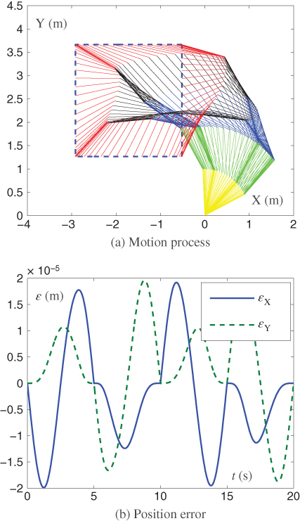
Figure 1.4 (a) Motion process and (b) position error of a five-link planar robot manipulator synthesized by the pseudoinverse-based MVN scheme (1.1) and aided by the TDTZD-U model (1.14).
For further comparison, numerical results synthesized by the pseudoinverse-based MVN scheme (1.1) aided with a EDTZD-U model (1.10) and Newton iteration (1.15) are shown in Figure 1.5. Note that, similar to Figure 1.3 and Figure 1.4 synthesized by TDTZD-U model (1.14), the joint-angle, joint-velocity, and motion process generated by Newton iteration (1.15) are omitted due to space limitation.
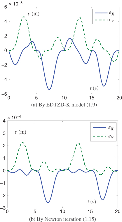
Figure 1.5 Position error of a five-link planar robot manipulator synthesized by a pseudoinverse-based MVN scheme (1.1) aided with the EDTZD-K model (1.9) or Newton iteration (1.15).
It can be seen from Figure 1.5(a) that the maximum position error synthesized by EDTZD-U model (1.10) is ![]() m, which is roughly three times larger than that TDTZD-U model (1.14) in Figure 1.4. Besides, the maximum position error synthesized by Newton iteration (1.15) is
m, which is roughly three times larger than that TDTZD-U model (1.14) in Figure 1.4. Besides, the maximum position error synthesized by Newton iteration (1.15) is ![]() m, which is roughly 10 times larger than that TDTZD-U model (1.14) in Figure 1.4.
m, which is roughly 10 times larger than that TDTZD-U model (1.14) in Figure 1.4.
This application to the motion generation of the five-link planar robot manipulator further illustrates the superiority of the presented discrete-time ZD models for time-varying matrix pseudoinversion applied to the redundancy resolution of robot manipulators.
1.3.2 Application to a Three-Link Planar Robot Manipulator
In this section, the presented EDTZD-K model (1.9) and EDTZD-U model (1.10) are applied to the kinematic control of a three-link planar robot manipulator via online solution of time-varying pseudoinverse. In this application, the lengths of the links are set as ![]() m, and the initial joint state
m, and the initial joint state ![]() rad. In addition, the end-effector of the three-link planar robot manipulator is expected to track a square path with the side length being 0.5 m, and the motion-task duration is 40 s. Also, feedback gain is set as
rad. In addition, the end-effector of the three-link planar robot manipulator is expected to track a square path with the side length being 0.5 m, and the motion-task duration is 40 s. Also, feedback gain is set as ![]() .
.
It is worth pointing out that the motion process and the profiles of joint-angle and joint-velocity are omitted due to space limitation and we only present the simulation results on position error. Besides, the figure on position errors generated by EDTZD-U model (1.10) is very similar to that generated by EDTZD-K model (1.9) and thus omitted here.
EDTZD-K model (1.9) is applied to the robot's kinematic control, with the results shown in Figure 1.6. As seen from the figure, better control precision can also be achieved by using EDTZD-K model (1.9) with appropriate values of step size ![]() and sampling period
and sampling period ![]() . That is, as synthesized by EDTZD-K model (1.9), the end-effector trajectories of the three-link planar robot manipulator are both sufficiently close to the desired square path with small position errors (i.e., of orders
. That is, as synthesized by EDTZD-K model (1.9), the end-effector trajectories of the three-link planar robot manipulator are both sufficiently close to the desired square path with small position errors (i.e., of orders ![]() and
and ![]() m). These substantiate the effectiveness of the discrete-time models on robots' kinematic control.
m). These substantiate the effectiveness of the discrete-time models on robots' kinematic control.

Figure 1.6 Position errors of a three-link planar robot manipulator synthesized by a pseudoinverse-based MVN scheme (1.1) aided with EDTZD-K model (1.9) with  .
.
1.4 Chapter Summary
In this chapter, discrete-time ZD models have been presented and investigated for application to kinematic control of redundant robot manipulators. Specifically, to obtain the theoretical pseudoinverse of time-varying Jacobian matrix involved in robotic redundancy resolution, the continuous-time ZD model (1.7) and different discrete-time ZD models have been developed and investigated. Theoretical results have also been given showing the ZD models' feasibility for redundant-manipulator kinematic control. Then, the presented discrete-time ZD models have been applied to different types of redundant robot manipulators (i.e., the five-link planar robot manipulator and the three-link planar robot manipulator). Simulation results have illustrated the effectiveness of the presented discrete-time ZD models for time-varying matrix pseudoinversion applied to the redundancy resolution of robot manipulators.