4
Transient and Dynamic Rheological Properties of Emerging Hydrocolloids
Ali Alghooneh and Seyed M.A. Razavi
Food Hydrocolloids Research Center, Department of Food Science and Technology, Ferdowsi University of Mashhad, Mashhad, Iran
4.1 Introduction
Exploring novel hydrocolloids provides additional flexibility in the design of new products that may have a lower cost. In this way, there is great interest in well‐characterized natural hydrocolloids with appropriate functionality. Fundamental rheological properties include elasticity, viscosity, and viscoelasticity, which are related to the composition, structure, and the strength of interaction within the structural elements of hydrocolloids [1]. Steady shear flow tests concern the flow properties of all fluids, regardless of whether or not they exhibit elastic behavior. Nevertheless, many rheological characteristics of hydrocolloids cannot be described by viscosity alone, and elastic function must also be taken into account. Experiments based on unsteady state deformations, such as oscillatory and transient tests, are implemented to generate data that reflect both the elastic and viscous characters of materials [2]. These tests can be performed in linear and nonlinear regions.
In any industry, the choice of hydrocolloids is based on their functions, which are associated with their molecular characteristics (e.g., molecular weight, conformation, flexibility, polarity, and hydrophobicity) and so with their rheological behaviors. Thus, introducing the rheological properties of novel hydrocolloids and questioning their similarity to the generally used hydrocolloids based on some specific rheological parameters could be beneficial to rationally design structural features in food systems and to give insight into the structure–function relationship between them. However, a definitive scheme does not exist to characterize biopolymers on the basis of their important structural properties obtained from dynamic and transient rheological measurements and to discover their similarity.
Clustering is a part of pattern recognition theory. It helps to summarize information by grouping data in categories in which the members are as similar as possible to each other in the same group and as different as possible from members of other categories. The hierarchical algorithm is one of the clustering techniques and is classified into agglomerative hierarchical and divisive hierarchical methods [3]. Agglomerative hierarchical clustering is appropriate to represent the original data set in the feature space at multiple levels of abstraction because of each clustering level produces an abstract representation of the original data set [3]. Clustering has been successfully applied in various fields of the food industry [ 3–5].
Guar gum (GG), pectin (PE), and xanthan gum (XG) are three generally used hydrocolloids in food formulations. GG is obtained from guar (Cyamopsis tetragonoloba) seeds. It contains linear chains of D‐mannopyranosyl units with a D‐galactopyranose substituent protruding by (1 → 6) linkages and has the specific structure of galactomannans with 1.3 × 10³ kDa molecular weight and 12.5 dl g−1 intrinsic viscosity [6]. XG is a high‐molecular‐weight exopolysaccharide (4.05 × 10³ kDa) produced by the bacterium Xanthomonas compestirs and consists of a cellulose backbone with an attached charged trisaccharide side chain composed of a glucuronic acid residue between two mannose residues [7]. Higiro et al. [7] reported 214.21 dl g−1 intrinsic viscosity for XG by using the Tanglertpaibul and Rao equation. PE, with a heteropolysaccharide structure, originates in most plant tissues, with α‐(1–4)‐D‐galacturonic acid units as the principal component, which interrupted by the insertion of rhamnose units and with side chains of neutral sugars attached to the backbone. Naturally, PE is highly methoxylated (HM) with more than 50% of the esterified carboxyl groups. The intrinsic viscosity of HM PE is 15 dl g−1 [8]. It has been reported that PE macromolecules adopt a slightly stiff conformation [9]. The literature establishes the high capability of both sage seed gum (SSG) and cress seed gum (CSG) for use in food formulations. SSG is extracted from Salvia macrosiphon seeds. The weight average molecular weight of SSG polysaccharides is 4 × 10²–1.5 × 10³ kDa [10,11]. It is a polyelectrolyte galactomannan (1.78–1.93:1 mannose/galactose ratio and 28.2%–32.2% uronic acids) with 22.55 dl g−1 intrinsic viscosity [11]. CSG exists in the outer layer of the garden cress plant seed (Lepidium sativum L.). CSG, with a molecular weight of 540 kDa, possesses a semi‐rigid chain conformation [12]. This polyelectrolyte galactomannan (8.2 mannose/galactose ratio, 15% uronic acids, and 13.3 dl g−1 intrinsic viscosity) is known as a novel thickening, gelling, and emulsifying agent [13–16].
To the best of our knowledge, there is no similar published work regarding the characterization of the biopolymers structure that widely addresses dynamic and transient rheological behaviors. Therefore, the aims of the present study were, broadly, investigation of three commercialized (GG, PE, and XG) and two novel hydrocolloids' (CSG and SSG) dynamic oscillatory rheological properties (small amplitude strain sweep, large amplitude strain sweep, frequency sweep, time sweep), transient rheological properties (creep and stress relaxation) and the Cox–Merz rule, yield stress, and finally, probing the similarity of these five hydrocolloids based on the aforementioned rheological properties using the hierarchical clustering technique and principal component analysis (PCA) in a serial mode. Such a comprehensive rheological investigation is critical to decide on the hydrocolloids on the basis of their specific usage in food formulations and other industries, to adjust processing parameters and is important from the fundamental point of view.
4.2 Viscoelastic Characteristics
4.2.1 Oscillatory Properties
4.2.1.1 Strain Sweep
Rheological measurements were carried out using a Physica MCR 301 rheometer (Anton Paar, GmbH, Graz, Austria) equipped with cone‐plate geometry (4° cone angle, 50 mm of diameter, and 1 mm gap). The temperature was fixed using a Peltier system at 20 °C, and then each sample was equilibrated for at least 5 min before the rheological test and was coated around their periphery with light silicone oil to minimize loss of water. Strain sweep tests in oscillatory shear were performed in the range 0.01%–250% in the controlled shear rate mode at 20 °C and a constant frequency of 1 Hz. Then, data in the linear viscoelastic region, LVE, and in the nonlinear viscoelastic region, NLVE, were analyzed.
4.2.1.1.1 Small Amplitude Oscillatory Shear Test
The storage modulus (G′ LVE ), complex modulus (G* LVE ), loss tangent (tan δ ) in LVE, limiting value of strain (γ c ) and stress (τ c ), the slope of loss tangent after flow point (tan δ AF ), the extent of strain overshoot (G″ p /G″ LVE ), fracture strain (γ Fr ), fracture stress ( τ Fr ), and degree of ductility ((γ Fr ‐γ L ) / γ Fr )) were determined by the amplitude sweep measurements [17]. These parameters of five selected hydrocolloids are presented in Table 4.1. With an increase in strain, two different regions were observed (data not shown): (1) LVE, where G′ and G″ were approximately constant, while G′ was greater than G″ and (2) NLVE, in which G′ and G″ started to decline. At LVE, the highest and lowest values of the elastic moduli of PE and CSG were 158.00 and 7.40 Pa, respectively. This parameter demonstrates the rigidity of the sample [18]. The complex modulus, G* LVE (comprising both elastic and viscose components), showed a similar trend with G′ LVE for all gums, indicated that the total structural strength of PE was at the highest extent. Tan (δ) LVE , which indicates the physical behavior of a system (the ratio of G″ LVE to G′ LVE ), of all samples was less than 1, although GG, with the highest value of this parameter, showed the most liquid‐like behavior, followed by CSG, while there were not any significant differences between PE, XG, and SSG, which suggested a more pronounced solid‐like behavior for them. The critical strain (γ c , the strain in which G′ sharply decreases with an increase in strain) of GG was the highest (33.00%), followed by CSG (9.10%), whereas PE exhibited the lowest value of this parameter among all (0.95%). On the other hand, γ c did not show any significant difference between SSG and XG. Γ c depends on the molecular architecture of the biopolymers [19] and the deformability of the gel samples [20]. This result suggested that the timescale of interaction in PE chains is much longer than those in GG, which increases the time required for a new entanglement to replace those disrupted by an externally imposed small deformation in the amplitude oscillatory test. The magnitude of the stress at the limiting strain, τ c (the nonlinear region immediately begins after this stress), which is considered as the starting point of the weakening of the gel strength, was in the order of PE > XG > SSG > GG ≈ CSG. With the increase in the strain being higher than the critical strain, the G′ of all gum dispersions decreased consistently. The G″ of GG and CSG showed a similar behavior with G′, whereas in XG, PE, and SSG, G″ showed overshoot. This suggests that the structures formed with the CSG and GG were weaker than those formed with XG, SSG, and PE [21]. Hyun [22] reported that at least four types of large‐amplitude oscillatory shear (LAOS) behavior exist depending on the interactions between the microstructures: type I, strain thinning (G′, G″ decreasing); type II, strain hardening (G′,G″ increasing); type III, weak strain overshoot (G′ decreasing, G″ increasing followed by decreasing); type IV, strong strain overshoot (G′,G″ increasing followed by decreasing). On the basis of this classification, XG, PE, and SSG showed weak strain overshoot behavior, whereas CSG and GG demonstrated strain thinning behavior. The former behavior, which has the same origin as shear‐thinning behavior, is most easily observed in polymer solutions and melts. With an increase in strain, polymer chains disentangle and align with the flow field. This response becomes more significant in anisotropic systems which flow more readily, and both moduli afterward decrease further [22]. On the other hand, a highly extended biopolymer with a polyelectrolyte nature such as SSG, XG, and PE align and associate (partly due to hydrogen bonding) to form a weakly structured material in solution. These complex structures resist deformation up to a certain strain where G″ increases to its highest value. This peak in G″ denotes the maximum energy dissipation (viscous response) and has been reported in soft glassy materials [23,24]. Then, this shear‐induced structure is destroyed by a larger deformation, after which the polymer chains align with the flow field, and G″ decreases. G″ p /G″ LVE , which shows the extent of G″ overshoot and is an index of structural resistance against deformation, was lower for SSG than for two other hydrocolloids with weak strain overshoot behavior, while no significant difference was observed between XG and PE. After γ c , when the material yields and/or fractures, G′ decreased rapidly. One method to determine fracture strain or stress is by plotting the product of the elastic modulus and strain (G′.γ) against the dynamic strain and looking for a maximum, which corresponds to the fracture point. As shown in Table 4.1, only systems with G″ max exhibited fracture stress and strain. Among them, XG showed the highest fracture strain (γ Fr ), while PE showed the lowest value of this parameter. On the other hand, the order of fracture stress ( τ Fr ) of hydrocolloids dispersions was PE > XG > SSG. Fracture properties are important in food systems as they mimic the response of foods to chewing and biting. Fracture takes place at the weakest parts of the gel network [25]. This result shows that the sensitivity of entanglement to deformation for the three hydrocolloids was in the order XG < SSG < PE, whereas the strength of the structure at fracture was in the order SSG < XG < PE. From the comparison of τ Fr and τ c , one can conclude that microscopic fracture of the three gum dispersions showed the same order as for macroscopic fracture. Also, results showed a higher reversible extensibility ahead of fracture for XG and SSG than for PE, whose higher (γ Fr −γ L )/ γ Fr value suggested the highest brittleness for PE. It has been shown that the magnitude of the flow point stress (when G′ = G″), which is related to the yield stress characteristic, is strongly correlated with the spreadability of many food products. Beyond the flow point, materials change from viscoelastic to elastoviscous behavior, where the materials display irrecoverable deformation [26]. Since it seems that spreadability is a kinetic property that manifests from the yield point, it should not be defined by just the yield stress value. Therefore, we defined the slope of the loss tangent, which corresponds to the rate of change of the viscous to elastic behavior, after the flow point stress (tan δ AF ) of different hydrocolloids as a representative parameter of the spreadability characteristic. According to Table 4.1, PE showed the highest value of tan δ AF , while the lowest spreadability was observed for both GG and CSG.
Table 4.1 Storage modulus (G′ LVE ), complex modulus (G* LVE ), limiting value of strain (γ c ), limiting value of stress (τ c ), and loss tangent (Tan (δ) LVE ) in the linear viscoelastic region, besides extent of loss modulus overshoot G″ p /G″ LVE , fracture stress (τ Fr ), fracture strain (γ Fr ), reversible extensibility ahead of fracture ((γ Fr ‐γ L )/γ Fr ), the slope of loss tangent after flow point (Tan (δ) AF ) for sage seed gum (SSG), cress seed gum (CSG), xanthan (XG), pectin (PE), and guar gum (GG) as determined by amplitude sweep tests (1 Hz, 20 °C).
| Gum | G′ LVE (Pa) | G* LVE (Pa) | γ c (%) | τ c (Pa) | Tan (δ) LVE (−) | G″ p /G″ LVE (−) | γ Fr (−) | (γ Fr ‐γ L ) / γ Fr (%) | τ Fr (Pa) | Tan (δ) AF (−) |
| XG | 75.90b ± 0.76 | 77.10b ± 0.91 | 7.14bc ± 0.41 | 6.85b ± 0.51 | 0.18c ± 0.01 | 1.88a ± 0.07 | 37.30a ± 2.38 | 80.90a ± 0.12 | 20.90b ± 0.81 | 0.26b ± 0.01 |
| GG | 25.00d ± 1.02 | 31.50d ± 0.96 | 33.00a ± 1.40 | 1.52d ± 0.25 | 0.74a ± 0.02 | — | — | — | — | 0.003d ± 0.00 |
| PE | 158.00a ± 1.75 | 160.00a ± 1.79 | 0.95d ± 0.07 | 8.57a ± 0.28 | 0.16c ± 0.01 | 2.01a ± 0.03 | 10.00c ± 0.21 | 72.70b ± 0.82 | 25.70a ± 1.57 | 0.35a ± 0.01 |
| SSG | 55.80c ± 0.56 | 56.70c ± 0.67 | 5.25c ± 0.30 | 3.75c ± 0.28 | 0.18c ± 0.01 | 1.57b ± 0.06 | 27.40b ± 1.75 | 80.90a ± 0.14 | 15.40c ± 0.60 | 0.19c ± 0.01 |
| CSG | 7.40e ± 0.19 | 7.83e ± 0.12 | 9.10b ± 0.49 | 1.75d ± 0.21 | 0.34b ± 0.04 | — | — | — | — | 0.01d ± 0.00 |
a–d: Means followed by the same letters in the same column are not significantly different (P > 0.05).
4.2.1.1.2 LAOS Test
Small amplitude oscillatory tests use a small strain amplitude and so have a limited resolution for distinguishing complex fluids with structural differences. Steady simple shear rate experiments provide little information about the microstructure. Unlike these tests, the LAOS test provides valuable information with high resolution which is useful to connect quantitative nonlinear measures with microstructure and to provide useful information about the behavior of materials during processing operations in which a large deformation for short time is encountered and the material does not reach steady state [23]. With the transformation from the LVE to the NLVE range, the physical interpretation of dynamic properties is no longer the same as those in the LVE range because of the generation of the nonlinear response stress, which is not a perfect sinusoid and, consequently, the viscoelastic moduli are not uniquely defined. Different nonlinear material coefficients can be extracted from LAOS tests depending on the employed method (Lissajous curves, Fourier transform rheology, stress decomposition, decomposition of characteristic waveforms, and analysis of parameters related to Fourier transform rheology) and the chosen frame of reference (i.e., time domain or deformation domain) [ 23,27]. The methods which have been used to calculate viscoelastic moduli can be grouped into two categories: full cycle methods and local methods. A full cycle method allows the average elasticity and dissipated energy at each imposed pair of LAOS coordinates ( γ 0 , ω) to be calculated from the first‐order Fourier or Chebyshev coefficients (intercycle nonlinearities). On the other hand, local methods allow the viscoelastic moduli at an instantaneous strain to be calculated (intracycle nonlinearities).
Here, first, LAOS flow was qualitatively investigated via waveform analysis by using elastic and viscous Lissajous–Bowditch plots (also called Lissajous plots) in which the total stress (τ/τ0) was plotted versus
γ/γ
0
and ![]() , respectively. To quantitatively determine the extent of nonlinearity, we used the G ″3/G ″1 and G′3/G′1 ratios calculated from the Fourier transform analysis in the time domain. The type of nonlinearity – intracycle strain softening and intracycle strain stiffening (in the strain domain) and intracycle shear thinning and shear thickening (in the strain rate domain) –was determined using the Ewolt et al. [28] local method. Besides, intercycle nonlinearities (intercycle strain softening, intercycle strain stiffening, intercycle shear thinning, and intercycle shear thickening) were determined by Fourier transform analysis to better distinguish the LAOS behavior of different hydrocolloids. In addition, on the basis of the Ewolt et al. [29] procedure, the perfect plastic dissipation ratio is used for identifying plastic behavior and quantifying how close a measured material response corresponds to rigid, perfect plastic yield stress behavior.
, respectively. To quantitatively determine the extent of nonlinearity, we used the G ″3/G ″1 and G′3/G′1 ratios calculated from the Fourier transform analysis in the time domain. The type of nonlinearity – intracycle strain softening and intracycle strain stiffening (in the strain domain) and intracycle shear thinning and shear thickening (in the strain rate domain) –was determined using the Ewolt et al. [28] local method. Besides, intercycle nonlinearities (intercycle strain softening, intercycle strain stiffening, intercycle shear thinning, and intercycle shear thickening) were determined by Fourier transform analysis to better distinguish the LAOS behavior of different hydrocolloids. In addition, on the basis of the Ewolt et al. [29] procedure, the perfect plastic dissipation ratio is used for identifying plastic behavior and quantifying how close a measured material response corresponds to rigid, perfect plastic yield stress behavior.
The Lissajous plots of GG, CSG, SSG, XG, and PE at 100% strain are shown in Figure 4.1. For all the samples at strains of 0.1% and 1% and for GG and CSG at these strains as well as 10% strain (i.e., within the LVR), the shape of the elastic and viscous Lissajous plots were perfectly elliptical, indicating ideal viscoelastic behavior. With an increase in strain at 10% and 100% strains for SSG, XG, and PE, and at 100% strain for GG and CSG, the shape of the elastic Lissajous plots changed from an ellipse to a parallelogram and the area encompassed by the plots increased, indicating the shift from elastic to viscous‐dominated behavior. Although, XG, SSG, and PE solutions at 10% and 100% strains displayed strain‐hardening behavior, the shapes of the nonlinear stress waveforms were markedly different, which originated from different microstructures. Particular shapes of the Lissajous plot relate to different microstructural features and correspond to borderline different rheological behaviors [24]. This behavior may be attributed to the stronger gel network structure of SSG, XG, and PE than CSG and GG achieved through their polyelectrolyte moiety and rigid conformation, resulting in less flexibility of the network and greater structural damage under large strains, which is reflected by the start of nonlinearity at the lower strain compared with CSG and GG. The inability of the structure to adapt to large strains would result in permanent structural deformation and the appearance of viscous‐like behavior [24].

Figure 4.1 Elastic and viscous Lissajous plots of SSG, (a, b) CSG, (c, d) GG, (e, f) PE, (g, h) and XG, (i, j) respectively, at 100% strain (1%‐1 Hz).
While visual investigations of Lissajous plots are helpful to give an overview of nonlinear viscoelastic responses, quantitative methods are also necessary for analyzing the nonlinear shear stress responses. To determine the extent of nonlinearity and the behavioral shifts of Lissajous plots, the stress response to an oscillatory strain input was written as a Fourier series to determine the third viscoelastic moduli (![]() and
and ![]() ) [30]. Then, the ratio of the third harmonic viscoelastic moduli to the first harmonic viscoelastic moduli,
) [30]. Then, the ratio of the third harmonic viscoelastic moduli to the first harmonic viscoelastic moduli, ![]() and
and ![]() , were investigated. Values of
, were investigated. Values of ![]() or
or ![]() reflect nonlinear viscoelastic behavior.
reflect nonlinear viscoelastic behavior. ![]() and
and ![]() ratios were greater than 0.01 for XG, SSG, PE, and CSG at 10% and 100% strains, while this occurred only at 100% strain for GG, indicating nonlinear behavior at these strains (Table 4.2). For all hydrocolloids, when the samples showed nonlinearity, the extent of nonlinear viscoelastic behavior increased with an increase in strain, as reflected by the greater values of these ratios at higher strain. The highest
ratios were greater than 0.01 for XG, SSG, PE, and CSG at 10% and 100% strains, while this occurred only at 100% strain for GG, indicating nonlinear behavior at these strains (Table 4.2). For all hydrocolloids, when the samples showed nonlinearity, the extent of nonlinear viscoelastic behavior increased with an increase in strain, as reflected by the greater values of these ratios at higher strain. The highest ![]() and
and ![]() ratios at 10% and 100% were obtained for PE. The
ratios at 10% and 100% were obtained for PE. The ![]() ratio did not show any significant differences between SSG and XG at both 10% and 100% strains. In addition, with an increase in strain, the differences between these ratios for CSG and GG vanished (Table 4.2).
ratio did not show any significant differences between SSG and XG at both 10% and 100% strains. In addition, with an increase in strain, the differences between these ratios for CSG and GG vanished (Table 4.2).
Table 4.2 Elastic and viscous parameters of sage seed gum (SSG), cress seed gum (CSG), xanthan (XG), pectin (PE), and guar gums (GG) at different strains in LAOS domain.
| Elastic parameters | Viscous parameters | ||||
| Gum | Strain |
|
|
|
|
| XG | 0.1 | 0.981c 1 ± 0.022 | 0.001c 1 ± 0.000 | 0.943a 1 ± 0.028 | 0.009c 1 ± 0.000 |
| 1 | 0.971c 1 ± 0.036 | 0.001c 1 ± 0.000 | 0.984a 1 ± 0.047 | 0.004c 1 ± 0.000 | |
| 10 | 3.426b 2 ± 0.064 | 0.084b 3 ± 0.004 | 0.741b 2 ± 0.063 | 0.053b 3 ± 0.005 | |
| 100 | 6.480a 3 ± 0.209 | 0.204a 2 ± 0.013 | 0.481c 2 ± 0.038 | 0.186a 2 ± 0.012 | |
| GG | 0.1 | 0.943a 1 ± 0.046 | 0.001b 1 ± 0.000 | 0.941a 1 ± 0.028 | 0.001b 1 ± 0.000 |
| 1 | 0.968a 1 ± 0.036 | 0.002b 1 ± 0.000 | 0.968a 1 ± 0.046 | 0.000b 1 ± 0.000 | |
| 10 | 0.969a 1 ± 0.043 | 0.001b 1 ± 0.000 | 0.965a 3 ± 0.082 | 0.005b 1 ± 0.000 | |
| 100 | 0.797b 1 ± 0.052 | 0.046a 1 ± 0.003 | 0.876b 4 ± 0.053 | 0.036a 1 ± 0.002 | |
| PE | 0.1 | 0.983c 1 ± 0.032 | 0.001c 1 ± 0.000 | 0.990a 1 ± 0.030 | 0.003c 1 ± 0.000 |
| 1 | 0.974c 1 ± 0.036 | 0.002c 1 ± 0.000 | 0.967a 1 ± 0.046 | 0.002c 1 ± 0.000 | |
| 10 | 4.291b 3 ± 0.084 | 0.135b 3 ± 0.006 | 0.534b 1 ± 0.045 | 0.115b 4 ± 0.010 | |
| 100 | 8.591a 4 ± 0.426 | 0.260a 3 ± 0.017 | 0.182c 1 ± 0.012 | 0.493a 3 ± 0.032 | |
| SSG | 0.1 | 0.984c 1 ± 0.012 | 0.002c 1 ± 0.000 | 1.057a 1 ± 0.032 | 0.002c 1 ± 0.001 |
| 1 | 1.062c 1 ± 0.040 | 0.003c 1 ± 0.000 | 0.947a 1 ± 0.043 | 0.004c 1 ± 0.001 | |
| 10 | 3.514b 2 ± 0.068 | 0.096b 3 ± 0.004 | 0.780b 2 ± 0.066 | 0.043b 3 ± 0.004 | |
| 100 | 5.485a 2 ± 0.161 | 0.174a 2 ± 0.011 | 0.577c 2 ± 0.045 | 0.081a 1 ± 0.005 | |
| CSG | 0.1 | 0.942a 1 ± 0.031 | 0.001b 1 ± 0.000 | 0.924a 1 ± 0.028 | 0.001b 1 ± 0.000 |
| 1 | 0.965a 1 ± 0.036 | 0.002b 1 ± 0.000 | 0.894a 1 ± 0.042 | 0.002b 1 ± 0.001 | |
| 10 | 0.933a 1 ± 0.042 | 0.012b 2 ± 0.000 | 0.861a 2 ± 0.073 | 0.022b 2 ± 0.002 | |
| 100 | 0.702b 1 ± 0.045 | 0.080a 1 ± 0.005 | 0.776b 3 ± 0.050 | 0.052a 1 ± 0.003 | |
1–5: Means followed by the same number in the same column denote that the corresponding parameter for each column is not significantly different among hydrocolloids at the same strain (P > 0.05).
a–d: Means followed by the same letter in the same column denote that the corresponding parameter for each column is not significantly different for each gum at various strains (P > 0.05).
The type of intracycle nonlinear behavior was identified by using two viscoelastic moduli, ![]() (the largest strain modulus) and
(the largest strain modulus) and ![]() (the minimum strain modulus), and two instantaneous viscosities,
(the minimum strain modulus), and two instantaneous viscosities, ![]() (the instantaneous viscosity at the largest strain rates) and
(the instantaneous viscosity at the largest strain rates) and ![]() (the instantaneous viscosity at the smallest strain rates) parameters defined by Ewoldt et al. [28].
(the instantaneous viscosity at the smallest strain rates) parameters defined by Ewoldt et al. [28].![]() and
and ![]() are the measures of elastic‐related nonlinear behavior and viscous‐related nonlinear behavior, respectively. These parameters for all hydrocolloids are depicted in Table 4.2. The magnitudes of the ratio of
are the measures of elastic‐related nonlinear behavior and viscous‐related nonlinear behavior, respectively. These parameters for all hydrocolloids are depicted in Table 4.2. The magnitudes of the ratio of ![]() – higher than 1, less than 1, and equal to unity – are indicative of strain‐stiffening, strain‐softening, and linear elastic behaviors, respectively. Furthermore,
– higher than 1, less than 1, and equal to unity – are indicative of strain‐stiffening, strain‐softening, and linear elastic behaviors, respectively. Furthermore,![]() indicates a linear regime,
indicates a linear regime, ![]() represents shear‐thinning behavior, and
represents shear‐thinning behavior, and ![]() indicates shear‐thickening behavior [28]. On the basis of these classifications, XG, PE, and SSG behaved similarly, with strain and their elastic components showing linear elastic behavior at 0.1% and 1% strains, while demonstrating strain‐stiffening behavior at 10% and 100%. Also, the amount of strain stiffening was greater at higher strains. At 10% and 100% strains, PE displayed the greatest amount of strain‐hardening behavior among the hydrocolloids. On the other hand, the elastic component of CSG and GG showed linear elastic behavior at 0.1%, 1%, and 10% strains, whereas they showed strain‐softening behavior at 100% strain.
indicates shear‐thickening behavior [28]. On the basis of these classifications, XG, PE, and SSG behaved similarly, with strain and their elastic components showing linear elastic behavior at 0.1% and 1% strains, while demonstrating strain‐stiffening behavior at 10% and 100%. Also, the amount of strain stiffening was greater at higher strains. At 10% and 100% strains, PE displayed the greatest amount of strain‐hardening behavior among the hydrocolloids. On the other hand, the elastic component of CSG and GG showed linear elastic behavior at 0.1%, 1%, and 10% strains, whereas they showed strain‐softening behavior at 100% strain. ![]() was almost equal to unity for XG, SSG, and PE at 0.1% and 1% strains, indicating linear viscous behavior of their viscose component. This behavior was shown for CSG and GG at 0.1%, 1%, and 10% strains.
was almost equal to unity for XG, SSG, and PE at 0.1% and 1% strains, indicating linear viscous behavior of their viscose component. This behavior was shown for CSG and GG at 0.1%, 1%, and 10% strains. ![]() ratio was less than unity for XG, SSG, and PE at 10% and 100% and for CSG and GG at 100% strain. The lowest values of these ratios were obtained for PE at both 10% and 100% strains, whereas the lowest shear‐thinning behavior at 10% strain was obtained for GG followed by CSG and at 100% for SSG and XG without any significant differences. These results indicated the higher sensitivity of SSG and XG, and especially PE gels, structure to a large deformation than the other two galactomannans [24].
ratio was less than unity for XG, SSG, and PE at 10% and 100% and for CSG and GG at 100% strain. The lowest values of these ratios were obtained for PE at both 10% and 100% strains, whereas the lowest shear‐thinning behavior at 10% strain was obtained for GG followed by CSG and at 100% for SSG and XG without any significant differences. These results indicated the higher sensitivity of SSG and XG, and especially PE gels, structure to a large deformation than the other two galactomannans [24].
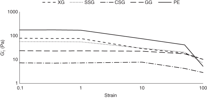
Figure 4.2
Strain independency of first harmonic elastic modulus  of sage seed gum (SSG), cress seed gum (CSG), xanthan (XG), pectin (PE), and guar gum (GG).
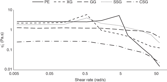
Figure 4.3
Strain independency of first harmonic viscose component  of sage seed gum (SSG), cress seed gum (CSG), xanthan (XG), pectin (PE), and guar gum (GG).
To gain a deeper insight into the rheological and structural behaviors of the selected hydrocolloids, the average elasticity and dissipated energy in the material response were determined by means of the full cycle method using Fourier series, and the results are shown in Figures 4.2 and 4.3, respectively. At 0.1%–1% strain, the elastic component of all hydrocolloids showed linear elastic behavior, reflected by the strain independency of the first harmonic elastic modulus (![]() ). With an increase in strain in the range 0.1%–10% and 0.1%–100%, the elastic modulus decreased with an increase in strain, indicating an intercycle strain‐softening behavior for all the studied systems. With an increase in the strain range at 0.1%–10%, the
). With an increase in strain in the range 0.1%–10% and 0.1%–100%, the elastic modulus decreased with an increase in strain, indicating an intercycle strain‐softening behavior for all the studied systems. With an increase in the strain range at 0.1%–10%, the ![]() reduction ratios of SSG, XG, and PE were not significantly different; similarly, CSG and GG did not show any significant differences in the
reduction ratios of SSG, XG, and PE were not significantly different; similarly, CSG and GG did not show any significant differences in the ![]() reduction ratio, although the former group showed a much higher reduction ratio than the latter one. Finally, at 0.1%–100%, the order of the
reduction ratio, although the former group showed a much higher reduction ratio than the latter one. Finally, at 0.1%–100%, the order of the ![]() reduction ratio was PE > XG ≈ SSG > CSG ≈ GG. Regarding the first harmonic viscous component behavior of different hydrocolloids, except GG and CSG, other gum dispersions exhibited a three‐stage first‐order dynamic viscosity versus shear rate response when sheared over a wide shear rate range. The intercycle shear‐thinning behavior was observed for all tested dispersions, which may be attributed to the formation of aggregated polymers dispersions and their high molecular weight [31]. With the exception of CSG and GG, at a lower strain rate, a shear‐thickening region appeared. This behavior was followed by the Newtonian plateau at the lowest strain rate range for all gum dispersions. The length of each region was quite different for all gum dispersions. PE showed the highest length of the shear‐thickening region, while XG showed the highest extent of shear‐thickening behavior. It is assumed that the shear‐thickening behavior could be the result of a stiffer inner structure with formation of entanglements of polymer coils as the shear rate increases [32]. This result suggested a greater effect of the shear rate on the thickening of PE and XG and the greater resistance of these hydrocolloids against the shear rate. Besides, different structure formation was exhibited with shear for PE and XG at low shear rates. On the other hand, CSG exhibited the highest length of Newtonian region among all gum dispersions, from 0.006 to 1.453 s−1. In the low‐shear Newtonian stage, the disrupted entanglement under deformation is replaced by new ones, whereas in the shear‐thinning stage, the chains undergo continuing rearrangement as the shear rate increases [33]. Shear thinning begins when the rate of disentanglement becomes greater than the rate of re‐formation [34]. This occurred at the same shear rate for PE and GG while they showed the highest value of this parameter. The extent of intercycle shear thinning was in the order PE > XG > SSG > CSG > GG, which confirmed the highest effect of shear on PE entanglement disruption at high shear rates. It is well known that when a small‐particle‐sized dispersion encountered shearing, the effect of Brownian motion lasts longer along the shear rate axis, and higher values of the shear rate are needed to initiate the shear‐thinning stage [35]. An abrupt
reduction ratio was PE > XG ≈ SSG > CSG ≈ GG. Regarding the first harmonic viscous component behavior of different hydrocolloids, except GG and CSG, other gum dispersions exhibited a three‐stage first‐order dynamic viscosity versus shear rate response when sheared over a wide shear rate range. The intercycle shear‐thinning behavior was observed for all tested dispersions, which may be attributed to the formation of aggregated polymers dispersions and their high molecular weight [31]. With the exception of CSG and GG, at a lower strain rate, a shear‐thickening region appeared. This behavior was followed by the Newtonian plateau at the lowest strain rate range for all gum dispersions. The length of each region was quite different for all gum dispersions. PE showed the highest length of the shear‐thickening region, while XG showed the highest extent of shear‐thickening behavior. It is assumed that the shear‐thickening behavior could be the result of a stiffer inner structure with formation of entanglements of polymer coils as the shear rate increases [32]. This result suggested a greater effect of the shear rate on the thickening of PE and XG and the greater resistance of these hydrocolloids against the shear rate. Besides, different structure formation was exhibited with shear for PE and XG at low shear rates. On the other hand, CSG exhibited the highest length of Newtonian region among all gum dispersions, from 0.006 to 1.453 s−1. In the low‐shear Newtonian stage, the disrupted entanglement under deformation is replaced by new ones, whereas in the shear‐thinning stage, the chains undergo continuing rearrangement as the shear rate increases [33]. Shear thinning begins when the rate of disentanglement becomes greater than the rate of re‐formation [34]. This occurred at the same shear rate for PE and GG while they showed the highest value of this parameter. The extent of intercycle shear thinning was in the order PE > XG > SSG > CSG > GG, which confirmed the highest effect of shear on PE entanglement disruption at high shear rates. It is well known that when a small‐particle‐sized dispersion encountered shearing, the effect of Brownian motion lasts longer along the shear rate axis, and higher values of the shear rate are needed to initiate the shear‐thinning stage [35]. An abrupt ![]() reduction occurred at 50% strain for PE, and this abrupt change occurred for
reduction occurred at 50% strain for PE, and this abrupt change occurred for ![]() reduction of XG (1.45 s−1) and PE (8.06 s−1) too, suggesting that these hydrocolloids assumed a more complicated structure. GG and CSG showed almost uniform
reduction of XG (1.45 s−1) and PE (8.06 s−1) too, suggesting that these hydrocolloids assumed a more complicated structure. GG and CSG showed almost uniform ![]() reduction at all strain ranges, suggested the least intercycle strain‐softening behavior among other gums.
reduction at all strain ranges, suggested the least intercycle strain‐softening behavior among other gums.
Rigid, perfectly plastic behavior is an idealized approximation for a material which exhibits slight elastic strains in comparison with large plastic deformations. This behavior can originate from strong short‐range interparticle forces which maintain a percolated solid phase and is observed for many “apparent yield stress fluids” [29]. To compare the energy dissipated in a single LAOS cycle to the energy which would be dissipated in a perfect plastic response, we employed the ϕ parameter as follows:

where E d is the energy dissipated per unit volume in a single LAOS cycle, visualized by the area enclosed by the Lissajous curve of stress versus strain, (E d ) pp is the energy dissipated per cycle by the perfect plastic in LAOS, and σ max is the maximum stress. With an increase in strain, the ϕ values of SSG, XG, and PE approach the yield stress limit ϕ → 1, while for CSG and GG, they almost were close to the Newtonian fluid reference value ϕ ≈ π/4 ≈ 0.785 (data not shown). The highest ϕ value was obtained for PE at 100% strain, which showed the closest response to that of a perfect plastic under LAOS deformations. At 100% deformation, ϕ did not show any significant differences between SSG and XG and also between CSG and GG. We analyzed the correlation between the loss tangent after flow point (tan δ AF ) data and plastic dissipation index (ϕ) data. These two parameters exhibited a significant linear positive correlation with each other (p < 0.05), indicating that a possible trend observed in one of these parameters can be estimated by the other. The presented data demonstrate that the analysis of the nonlinear behaviors of hydrocolloids may be successfully carried out with the use of the LAOS techniques.
4.2.1.2 Frequency Sweep
Dynamic measurements were performed over the frequency range 0.01–10 Hz within the LVE range (strain amplitude 0.50%). In this frequency range, except for GG, the G′ dominating over the G″ with weak frequency dependence and the mechanical spectra did not show any crossover points for all the hydrocolloids. The frequency at which G′ becomes equal to G″ is called the crossover frequency (f*) and is considered as the beginning of the elastic plateau. f* was 5.130 Hz for GG. To investigate the possible crossover points outside the experimental frequency range for other gum dispersions, we asymptote two lines from the end of G′ and G″ versus the frequency curves. PE showed the lowest f*, followed by SSG and XG without any significant differences (Table 4.3). When the frequency is so high that translational movements are no longer feasible, they start behaving like the weak gels, with G′ greater than G″ and exhibiting little change with frequency [36]. This result suggested the lowest entanglement density for GG and the strongest associated network for PE among all the hydrocolloids.
Table 4.3 Frequency dependency of the elastic (k′ and n′), loss (k″ and n″) and complex (A and z) moduli, the complex viscosity slope (η* s ), the molecular weight between crosslinks (M c ), degree of crosslinking (X c ), number density of crosslinks (υ), the distance between sequential crosslinking points (ξ), elastic active network chain (EANC) concentration, and the crossover frequency (f*) (1% w/w, 0.5% strain).
| Gum | k′ | n′ | k″ | n″ | k″/k′ | η* s | A | z | M c | X c | υ | ξ | EANC | f* |
| XG | 52.01b ± 1.07 | 0.15c ± 0.01 | 11.31b ± 0.11 | 0.08c ± 0.01 | 0.22c ± 0.00 | −0.82c ± 0.02 | 54.10b ± 0.17 | 6.41c ± 0.17 | 52848.3c ± 205.7 | 1.88 × 10⁻⁵b ± 7.33 × 10⁻⁸ | 1.74 × 10²²b ± 6.76 × 10¹⁹ | 3.85 × 10⁻⁸c ± 1.50 × 10⁻¹⁰ | 0.027b ± 0.002 | 0.002c ± 0.000 |
| GG | 4.79d ± 0.17 | 0.72a ± 0.04 | 8.32c ± 0.10 | 0.47a ± 0.02 | 1.67a ± 0.04 | −0.46a ± 0.02 | — | — | — | — | — | — | — | 5.130a ± 0.143 |
| PE | 120.43a ± 1.27 | 0.12c ± 0.01 | 18.29a ± 0.39 | 0.07c ± 0.01 | 0.15d ± 0.00 | −0.87d ± 0.03 | 131.42a ± 1.27 | 9.30a ± 0.06 | 27100.7d ± 145.2 | 3.66 × 10⁻⁵a ± 1.96 × 10⁻⁷ | 3.53 × 10²²a ± 1.89 × 10²⁰ | 3.03 × 10⁻⁸d ± 1.63 × 10⁻¹⁰ | 0.055a ± 0.053 | 0.000d ± 0.000 |
| SSG | 36.47c ± 0.75 | 0.11c ± 0.00 | 8.05c ± 0.08 | 0.13c ± 0.01 | 0.22c ± 0.00 | −0.85c ± 0.02 | 39.79c ± 0.47 | 7.31b ± 0.29 | 90283.5b ± 413.7 | 1.10 × 10⁻⁵c ± 5.04 × 10⁻⁸ | 9.69 × 10²¹c ± 4.44 × 10¹⁹ | 4.67 × 10⁻⁸b ± 2.14 × 10⁻¹⁰ | 0.016b ± 0.002 | 0.002c ± 0.000 |
| CSG | 4.65d ± 0.18 | 0.40b ± 0.03 | 1.94d ± 0.06 | 0.30b ± 0.01 | 0.42b ± 0.03 | −0.63b ± 0.01 | 4.88d ± 0.05 | 2.67d ± 0.06 | 142588.4a ± 1491.0 | 6.91 × 10⁻⁶d ± 7.23 × 10⁻⁸ | 6.04 × 10²¹d ± 6.32 × 10¹⁹ | 5.44 × 10⁻⁸a ± 5.69 × 10⁻¹⁰ | 0.010c ± 0.000 | 0.038b ± 0.002 |
a–d: Means followed by the same letters in the same column are not significantly different (P > 0.05).
The effect of frequency ranges on the decreasing percentage and decreasing ratio of the dynamic viscosity (η′) of different gum dispersions was investigated to find out the pseudoplasticity of hydrocolloids in the dynamic shear rheological test in the small deformation mode (data not shown). It was found that, except for GG, which showed the highest percentage of viscosity reduction at both 0.628–6.280 and 6.280–62.800 rad s−1, for all other gum dispersions this phenomenon occurred at 0.0628–0.6280 rad s−1. At the lowest angular frequency range (0.0628–0.6280 rad s−1), the η′ reduction percentage did not show any significant difference between SSG, XG, and PE; besides, these hydrocolloids showed a higher η′ reduction percentage than GG and CSG. In addition, PE with the highest η′ ratio reduction at all three angular frequency ranges (0.0628–0.6280, 0.0628–6.2800, and 0.0628–62.800 rad s−1) represented the highest shear‐thinning behavior, while there were no significant differences between GG and CSG, the gums least influenced by shear at all these ranges. Shear thinning as an important rheological behavior of biopolymers is found to be broadly different in steady and dynamic shear tests [37]. In contrast to the steady shear test (under a large deformation), in which shear thinning occurs when rod‐like particles are aligned in the flow direction and have lost their junctions in polymer solutions, in the dynamic test at high frequency when the time interval is not large enough for the broken inter‐ and intramolecular bonds to re‐form, permanent disentanglement of long‐chain polymers occurs, causing a decrease in η′. Therefore, this result shows that the timescale of segment–segment interaction in PE chains must be long in comparison with the lifetime of the physical entanglements of other hydrocolloids, which consequently leads to an increase in the time required for a new entanglement to replace those disentangled by the externally imposed deformation in the dynamic shear test.
The power‐law model (Eqs. 4.2 and 4.3) was used to estimate the frequency dependence of G′ and G″ from a double logarithmic plot of G′ and G″ against frequency as follows:
where k′ (Pa sn) and k″ (Pa sn) are intercepts, n′ and n″ are exponents or slopes of frequency dependence of G′ and G″, respectively, and ω is the angular frequency (rad s−1).
The correlation (R 2 value) between frequency and G′ or G″ was high for all gum dispersions (0.891–0.953). It was found that all gums displayed gel‐like behavior because the slopes (n′ = 0.110–0.725 and n″ = 0.694–0.469) were positive and were much lower than those reported for a Maxwell fluid (G′ ∞ ω 2 and G″ ∞ ω). A similar trend was observed for both n′ and n″ with respect to the gum type, in which GG showed the highest and SSG, XG, and PE, without any significant differences among them, showed the lowest values of both parameters. A low n′ value indicates elastic gel behavior, while for n′ values close to 1, the system behaves as a viscous gel [37]. This result suggests the general tendency of all dispersions to elastic gel, except for GG with a n′ of 0.725. The highest and lowest values for both k′ and k″ parameters were obtained for PE and CSG, respectively. This parameter represents the stiffness of the continuous phase due to the thickening effect of the hydrocolloid. The magnitudes of k′ were much higher than k″ for all gums, confirming the gel‐like behavior of these systems, except for GG, which showed the opposite trend, as reflected by the k′/k″ ratio of 1.674.
Based on a double logarithmic scale, the complex dynamic viscosity (η*) of all gum samples decreased linearly with increasing frequency, indicating a non‐Newtonian shear‐thinning flow behavior. The highest value of the complex viscosity slope (η* s ) was observed for PE (−0.867). Such behavior has been reported for XG, which creates a “weak‐gel” network by the tenuous association of rigid, ordered molecular structures in solution [38,39]. In a similar way, the η* s value for SSG and XG was substantially steeper than the maximum value of −0.76 which Morris [38] used to describe the “weak gel” characteristics of a polysaccharide gel formed by overlapping and entangled flexible random coil chains, whereas this parameter was −0.632 and −0.465 for CSG and GG, respectively. This result suggested strong shear‐thinning flow behavior for PE, XG, and SSG, which can be explained in terms of higher entanglement formation as they take on a rigid conformation in solution [ 6, 7, 9], while GG and CSG adopt random coil and semi‐rigid conformations, respectively, with a less entangled polymer solution [ 10, 11].
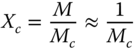
Except for GG, which showed concentrated solution rheological behavior, the network parameters of other hydrogel‐forming hydrocolloids were determined and reported in Table 4.3. In this way, the molecular weight between crosslinks, M c , the degree of crosslinking, X c , the number density of crosslinks, υ, and the distance between sequential crosslinking points, ξ, can be calculated according to the following equations, using the frequency sweep data [40]:


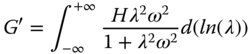
where ρ is the density (kg m−3), R is the gas constant (J mol−1 K−1), T is the temperature (K), G′ p is the plateau storage modulus (Pa), N A is the Avogadro number (atoms/mole), and M is the molecular weight (g mol−1). CSG showed the highest M c and ξ values, whereas PE showed the lowest values of these parameters. On the other hand, the X c and υ of these two gums showed the opposite trend. Other hydrocolloids showed intermediate values for these parameters. The υ of the semi‐crystalline and amorphous hydrogels vary, because semi‐crystalline gels had additional net points by crystallite formation, which resulted in a greater distance between sequential crosslinking points [41]. These results suggested the highest gel strength for PE occurs with the highest number density of crosslinks and degree of crosslinking and the lowest distance occurs between sequential crosslinking points. To understand the strength of the network and the network extension, dynamic data were explained by a power‐law relationship between the dynamic complex modulus (G*, Pa) and the frequency (ω, rad s−1) as follows [42]:
where z is the network extension, related to the number of interacting rheological units within the network (a higher z value corresponds to a more extended network), and A is the strength of the interactions (Pa s1/z). Except for GG, which did not have a weak gel structure, the z and A parameters of other hydrocolloids were calculated, and the results are depicted in Table 4.3. PE and CSG showed the highest and the lowest values of the z parameter, respectively. The A parameter of different gum systems showed a similar trend as the X c and υ parameters, suggesting that the strength of the interactions and the number of interacting rheological units increased along with the number and density of subunits groups contributing to crosslinking and vice versa.
The pseudo‐equilibrium modulus, G e , is a numerical measure of the structural contribution of the mechanical modulus. G e is defined as follows [43]:
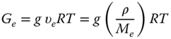
where g is a numerical factor, υ e is the moles of network stands per unit volume, ρ is the density, M e is the average molecular weight between crosslinks, R is the universal gas constant, and T is the absolute temperature. υ e , which is called the elastic active network chain (EANC) concentration, is directly proportional to the equilibrium modulus, and it quantitatively represents the structural contribution to the mechanical modulus. Generally, the numerical factor (g) is supposed to be unity. Then, from the plateau region of the frequency spectrum, G e and υ e (EANC) are estimated [43]. The EANC parameter was not accessible for GG, since this hydrocolloid did not demonstrate gel‐like behavior. The highest value of EANC was observed for PE, followed by SSG and XG without any significant differences between the latter gums (Table 4.3).
Table 4.4 Relaxation spectrum and fracture parameters of sage seed gum (SSG), cress seed gum (CSG), xanthan (XG), pectin (PE), and guar gum (GG).
| Gum | H(λ min ) (Pa) | d(Hλ)/dλ (Pa s−1) | C p (Pa) | Hλ max /Hλ min |
| XG | 11.157b ± 0.568 | 2.630d ± 0.133 | 0.724b ± 0.036 | 0.725a ± 0.037 |
| GG | 10.518b ± 0.378 | 4.564c ± 0.072 | 0.199d ± 0.016 | 0.053c ± 0.002 |
| PE | 35.665a ± 0.205 | 12.099a ± 0.359 | 2.492a ± 0.030 | 0.499b ± 0.018 |
| SSG | 8.520c ± 0.057 | 2.233d ± 0.083 | 0.596c ± 0.022 | 0.575b ± 0.019 |
| CSG | 10.518b ± 0.378 | 4.564c ± 0.072 | 0.199d ± 0.016 | 0.053c ± 0.002 |
a–d: Means followed by the same letters in the same column are not significantly different (P > 0.05).
4.2.1.2.1 Continuous Relaxation Spectrum
Timescales of various molecular motions can be plotted on a relaxation spectrum that describes chain dynamics [44]. The Generalized Maxwell model assumes that instead of a single relaxation time, the fluid has a distribution of relaxation times. If the number of elements in the Generalized Maxwell model is increased to infinity, a continuous spectrum is obtained as follows [45]:
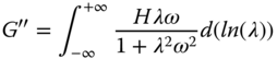
where H ( λ) is the continuous relaxation spectrum. The Tschoegl method was used to solve Eqs. 4.10 and 4.11 [46]. As the ±∞ limits of frequency were not accessible, the relaxation spectrum was determined in the operational frequency range of this study (0.01–10 Hz). Table 4.4 represents a number of valuable parameters obtained from the relaxation spectra of different gum dispersions. Macromolecular motion, also called structural relaxation, is accompanied by a reduction in chain stiffness, and thus mechanical network strength [44]. The relaxation time function of all gum dispersions slightly decreased with the increase in relaxation time up to a critical relaxation time point, C p (t), which marks the passage to a short‐time behavior and usually indicated the onset of the glassy state [44], followed by an abrupt reduction in the relaxation time function in which the discrepancies in spectral decay are distinguished well. This parameter was the highest for PE (2.492 s) and the lowest for GG (0.086 s), while other hydrocolloids showed intermediate C p values (Table 4.4). A similar trend was obtained for λ min with respect to the gum type. The structure corresponding to solid‐like behavior is responsible for the short relaxation times (λ min ). It is theorized that the microstructural features of the gel network that are responsible for the short relaxation times include the suprafibers, and the relaxation processes taking place in the junctions will correspond to longer relaxation times [45]. In the other words, slow movements (at long relaxation times) are due to the repetition of the entire chain along its contour [44]. Other valuable parameters which could be obtained from the relaxation spectra are the proportion of the relaxation strengths at long relaxation times (λ max ) to the relaxation strengths at short relaxation times (λ min ), (Hλ max /Hλ min ), which shows the extent of network strength change; and d(Hλ)/dλ, which represents the rate of mechanical network strength change with relaxation time. SSG and XG showed the lowest d(Hλ)/dλ value, while PE showed the highest d(Hλ)/dλ parameter, which demonstrated that although PE had the highest EANC and the lowest distance between sequential crosslinking points (ξ) (Table 4.3), the stiffness of its network is more unstable and decreases at a greater rate than SSG and XG. On the other hand, d(Hλ)/dλ was the highest for XG and the lowest for GG and CSG (without any significant differences between them). These results showed that the relaxation strengths at short relaxation times, the extent of network strength, and the kinetic parameters of network strength change (C p and d(Hλ)/dλ) differ with respect to the gum type, which suggests different spatial arrangements (aligned or non‐aligned hydrocolloids chains).
4.2.2 Transient Properties
4.2.2.1 Creep Test
The creep test was carried out at 0.1 Pa (the minimum stress for the linear viscoelastic domain) for 400 s, and the shear strain (![]() ) was recorded for a further 600 s during the recovery procedure. It is worth mentioning that the lower limit of the stress to achieve the linear viscoelastic domain in the creep compared to the dynamic rheology test (0.5 Pa) may be attributed to the different time frames of the dynamic and transient rheological tests. The creep and recovery compliances (J
C
and J
R
) were fitted by means of the four‐component Burger model (Eq. 4.12) and an empirical model (Eq. 4.13) for creep and recovery phases, respectively, as follows [47]:
) was recorded for a further 600 s during the recovery procedure. It is worth mentioning that the lower limit of the stress to achieve the linear viscoelastic domain in the creep compared to the dynamic rheology test (0.5 Pa) may be attributed to the different time frames of the dynamic and transient rheological tests. The creep and recovery compliances (J
C
and J
R
) were fitted by means of the four‐component Burger model (Eq. 4.12) and an empirical model (Eq. 4.13) for creep and recovery phases, respectively, as follows [47]:
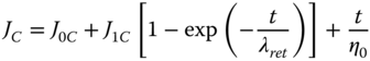
where J 0C is the instantaneous elastic compliance (Pa−1) of the Maxwell spring, J 1C is the elastic compliance (Pa−1) of the Kelvin–Voigt unit, λ ret is the retardation time (in seconds) of the Kelvin–Voigt component, and η 0 is the Newtonian viscosity (Pa s) of the Maxwell dashpot. b is the order of reaction, and a is the parameter that defines the recovery speed of the system. J ∞ and J 1R are the recovery compliances of the Maxwell dashpot and Kelvin–Voigt elements, respectively. When t → 0, J R is equal to J ∞ + J 1R , which corresponds to the maximum deformation of the dashpots in the Burger model. For t → ∞, J R is equal to J ∞, as it corresponds to the irreversible sliding of the Maxwell dashpot. The initial shear compliance, J 0R , was obtained by Eq. 4.14 as follows [48]:
where J max is the maximum compliance for the longest time (300 s) in the creep transient analysis. Full mechanical characterization of a system can be established by calculating the contribution of the compliances in Eqs. 4.12 and 4.13 to the maximum deformation to which the system is subjected. The percentage deformation of each element of the system can be calculated by

where J e is the corresponding compliance: J 0C , J 1C , J 0R , J 1R, , and J ∞ . In this chapter, the percentage deformation of η 0 was also determined by the following relationship:
In addition, the final percentage recovery (%R) of the entire system was calculated by the following equation [48]:
Table 4.5 Maximum compliance and the creep/recovery normalized parameters obtained for sage seed gum (SSG), cress seed gum (CSG), xanthan (XG), pectin (PE), and guar gum (GG).
| Creep | Recovery | ||||||||||
| Paramete r | XG | SSG | PE | GG | CSG | XG | SSG | PE | GG | CSG | |
|
|
0.25b 1 ± 0.01 | 0.21c 1 ± 0.01 | 0.30a 2 ± 0.01 | 0.01e 1 ± 0.00 | 0.16d 1 ± 0.01 |
|
0.25b 1 ± 0.01 | 0.31c 1 ± 0.01 | 0.35a 2 ± 0.01 | 0.01e 1 ± 0.00 | 0.17d 1 ± 0.01 |
|
|
0.50b 2 ± 0.01 | 0.47b 3 ± 0.02 | 0.56a 3 ± 0.04 | 0.18d 2 ± 0.03 | 0.40c 2 ± 0.00 |
|
0.42ab 2 ± 0.01 | 0.30c 1 ± 0.01 | 0.47a 3 ± 0.02 | 0.19d 2 ± 0.08 | 0.36c 2 ± 0.04 |
|
|
0.25c 1 ± 0.01 | 0.32bc 2 ± 0.02 | 0.14d 1 ± 0.06 | 0.81a 3 ± 0.03 | 0.42b 2 ± 0.05 |
|
0.27c 1 ± 0.00 | 0.39b 2 ± 0.00 | 0.17c 1 ± 0.03 | 0.80a 3 ± 0.08 | 0.47b 3 ± 0.04 |
| η 0 (Pa s) | 8773b ± 751 | 2432c ± 389 | 11730a ± 1600 | 38e ± 1 | 569d ± 88 | a | 0.09b ± 0.02 | 0.08b ± 0.01 | 0.14a ± 0.01 | 0.01d ± 0.00 | 0.05c ± 0.01 |
| λ ret (s) | 18.04b ± 3.85 | 13.76b ± 0.85 | 11.44b ± 1.07 | 115.57a ± 15.75 | 24.05b ± 0.56 | b | 0.62a ± 0.03 | 0.62a ± 0.02 | 0.63a ± 0.03 | 0.67a ± 0.02 | 0.66a ± 0.03 |
| J Max (1 Pa−1) | 0.07d ± 0.00 | 0.33c ± 0.00 | 0.07d ± 0.00 | 12.50a ± 0.57 | 1.55b ± 0.06 | %R | 73.10b ± 0.05 | 61.10c ± 0.15 | 82.81a ± 2.63 | 14.79e ± 8.54 | 46.72d ± 1.32 |
| R 2 adj | 0.967 | 0.930 | 0.972 | 0.999 | 0.950 | R 2 adj | 0.998 | 0.999 | 0.999 | 0.821 | 0.999 |
| RMSE | 0.003 | 0.026 | 0.003 | 0.040 | 0.083 | RMSE | 0.000 | 0.001 | 0.002 | 0.881 | 0.002 |
a–d: Means followed by the same letters in the same column are not significantly different (P > 0.05).
When the stress was applied, there was an instantaneous increase in strain, followed by a gradual increase over time for all samples, which can be attributed to the rearrangement of the network structure. The initial recovery corresponds to the spring of the Maxwell element (J
0R
), while the gradual increase in strain is the recovery due to the Kelvin–Voigt element (J
1R
). In the end, a residual or permanent deformation due to the irreversibility of the Maxwell dashpot sliding is depicted [49]. Compliance curves for creep and recovery phases of all hydrocolloids were successfully fitted with the Burger model (R2 ≥ 0.821 and RMSE ≤ 0.881) and the empirical model (R2 ≥ 0.89 and RMSE ≤ 0.05), respectively, and the resultant parameters are summarized in Table 4.5. GG showed the highest maximum compliance (J
max
), whereas PE and XG showed the lowest value of this parameter, indicating the greatest strength of the structure for the latter hydrocolloids. The most important contribution of the Maxwell spring to deformation, at creep (J
0C
≈ 30.40%) and recovery (![]() ), were those corresponding to the PE, while GG showed the lowest value of these parameters (Table 4.5). J
0C
represents the value of the instantaneous shear creep compliance at the initial time, and it may be related to the undisturbed hydrocolloid network structure and gel rigidity [50]. This is in agreement with the results earlier observed for the G′
LVE
behavior, in which PE showed the highest value of this parameter (Table 4.1). η
0, which represents the Newtonian flow viscosity, was the lowest for GG (38 Pa s) followed by CSG (569 Pa s) and the highest for PE (11730 Pa s). The contribution of the Maxwell dashpot to deformation at the creep (J
2C
*
) and recovery stages (
), were those corresponding to the PE, while GG showed the lowest value of these parameters (Table 4.5). J
0C
represents the value of the instantaneous shear creep compliance at the initial time, and it may be related to the undisturbed hydrocolloid network structure and gel rigidity [50]. This is in agreement with the results earlier observed for the G′
LVE
behavior, in which PE showed the highest value of this parameter (Table 4.1). η
0, which represents the Newtonian flow viscosity, was the lowest for GG (38 Pa s) followed by CSG (569 Pa s) and the highest for PE (11730 Pa s). The contribution of the Maxwell dashpot to deformation at the creep (J
2C
*
) and recovery stages (![]() ) were the highest for GG followed by CSG and SSG, indicating the lowest resistance to flow at longer times for GG [51]. Also, the viscosity flow deformation percentage in creep/recovery processes (J
2C
*
and
) were the highest for GG followed by CSG and SSG, indicating the lowest resistance to flow at longer times for GG [51]. Also, the viscosity flow deformation percentage in creep/recovery processes (J
2C
*
and ![]() ) played the most important role for GG among other compliances. The retarded compliance (J
1C
) represents the component of the viscoelastic behavior. So, the highest value of this parameter in the creep/recovery processes for PE and the lowest values for GG are associated with a greater elasticity of the Kelvin–Voigt element in the former and latter systems, respectively. In addition, J
1C
and
) played the most important role for GG among other compliances. The retarded compliance (J
1C
) represents the component of the viscoelastic behavior. So, the highest value of this parameter in the creep/recovery processes for PE and the lowest values for GG are associated with a greater elasticity of the Kelvin–Voigt element in the former and latter systems, respectively. In addition, J
1C
and ![]() were the most important compliances for PE at the creep and recovery stages, respectively. There were no significant differences among XG, PE, SSG, and CSG, while GG showed a higher value of the retardation time (λ
ret
). The Voigt unit represents an orientation of intermeshed macromolecules during which secondary bonds are breaking and re‐forming [52]. GG takes on a random coli conformation with less chain stiffness than XG, PE, SSG (rigid), and CSG (semi‐rigid) [ 6, 7, 9, 10, 12], which leads to a less entangled macromolecule with a shorter timescale of segment–segment interaction than other gums. This structure requires a shorter time for new entanglements to replace those disrupted by an externally imposed deformation, which results in a higher retardation time. This also implies that retardation time is inversely related to network viscoelasticity; that is, the lower the level of λ
ret
, the higher the elastic character of the sample [11]. The order of the recovery reaction (b parameter) was almost the same for all gums, while the speed of the recovery phase (a parameter) was the highest for PE and the lowest for GG, while other hydrocolloids showed intermediate values of the a parameter. The final percentage recovery behaved similarly to the a parameter. The higher the final percentage recovery value (%R), the higher the viscoelastic solid property of the sample [53]. In PE with the highest %R, only 17.19% of the links were irreversibly broken during the creep test.
were the most important compliances for PE at the creep and recovery stages, respectively. There were no significant differences among XG, PE, SSG, and CSG, while GG showed a higher value of the retardation time (λ
ret
). The Voigt unit represents an orientation of intermeshed macromolecules during which secondary bonds are breaking and re‐forming [52]. GG takes on a random coli conformation with less chain stiffness than XG, PE, SSG (rigid), and CSG (semi‐rigid) [ 6, 7, 9, 10, 12], which leads to a less entangled macromolecule with a shorter timescale of segment–segment interaction than other gums. This structure requires a shorter time for new entanglements to replace those disrupted by an externally imposed deformation, which results in a higher retardation time. This also implies that retardation time is inversely related to network viscoelasticity; that is, the lower the level of λ
ret
, the higher the elastic character of the sample [11]. The order of the recovery reaction (b parameter) was almost the same for all gums, while the speed of the recovery phase (a parameter) was the highest for PE and the lowest for GG, while other hydrocolloids showed intermediate values of the a parameter. The final percentage recovery behaved similarly to the a parameter. The higher the final percentage recovery value (%R), the higher the viscoelastic solid property of the sample [53]. In PE with the highest %R, only 17.19% of the links were irreversibly broken during the creep test.
4.2.2.2 Stress Relaxation Test
The rheological properties which are determined by the stress relaxation test are related to the properties of crosslinking in gel networks [54]. The stress relaxation test was made at a constant strain of 0.3%, and 25 °C, and the stress was recorded for 400 s. In order to predict the different patterns of viscoelasticity, the stress relaxation data were reduced to viscoelastic parameters by fitting an appropriate model to the stress‐time experimental data. Three common viscoelastic models, that is, the Generalized Maxwell (Eq. 4.18), Peleg (Eq. 4.19), and Nussinovitch (Eq. 4.20) were used as follows [47]:

where σ t is the time‐dependent stress, σ e is the stress in the elastic element, σ i is the stress in the combined viscous‐elastic elements, t is time, and τ i is the relaxation time of the combined viscous‐elastic elements. The Nussinovitch model is a simplified Generalized Maxwell model which assumes 10, 100, and 1000 as the relaxation times of the first, second, and third dashpot elements in the model. This model has been formulated for three viscous elements as follows [55]:
where σ 0 is the initial stress, t is time, and A 1 , A 2 , A 3 are constants. Peleg [56] proposed an empirical model as follows:
where the equilibrium stress, σ e , is calculated as
The constants k 1 and k 2 are obtained by linear regression. The advantages of this model are that if the data follow the linear relationship shown in Eq. 4.20, constants k 1 and k 2 will be independent of the test duration; also, this model predicts the complex behavior of materials (nonlinearity) well [57]. The Peleg model is the best approach for all the hydrocolloids (R2 = 0.912–0.976 and RMSE = 0.015–0.065) employed for data modeling of stress relaxation data, and the corresponding data are represented in Table 4.6. The stress relaxation rate, that is, the initial decay rate, is represented by the constant 1/ k 1 values. The initial decaying rate was the highest for GG followed by CSG, while there were no significant differences between the other three hydrocolloids. The physical significance of the k 1 value ought to be interpreted with caution since many materials initially relax fast; in addition, the shape of the very initial part of the recorded relaxation curves is strongly influenced by the deformation history of the sample. On the other hand, the value of k 2 is more indicative of the general rheological characteristics of materials. 1/ k 2 differed among hydrocolloids in the following order: GG ≈ CSG > SSG > XG ≈ PE. It is reported that k 2 represented the degree of solidity, and it varies between the value of k 2 = 1 for a material that is truly a liquid (i.e., all the stress relaxes) to k 2 → ∞ for an ideal elastic solid where the stress does not relax at all [57]. The reciprocal of k 2 denotes the asymptotic value of the relaxed portion of the initial stress and represents the portion of the stress that would have remained unrelaxed at equilibrium [56]. This result suggests more solid‐like behavior for PE and XG, whereas GG and CSG showed liquid‐like behavior in the stress relaxation test time scale. According to Table 4.6, σ e was the highest for XG and PE, whereas it was the lowest for GG. The equilibrium stress following relaxation is positively related to gel strength and reflects the degree of crosslinking in the polymer network [54]. It was reported that the relaxation time is the time required for the viscoelastic material to dissipate its force to about 36.8% (1/e) of the original applied force [58]. Accordingly, we supposed that when the stress reached the 1/e value of σ 0 , the materials yielded, and this time was reported as the relaxation time (λ). This parameter differed from the 1/ k 1 parameter, as the latter parameter concerns just the time dependency at t = 0, while the former one shows the total time dependency of the samples' structure during the test and is a measure of how fast the structure relaxes. The λ parameter varied among hydrocolloids in the following order: PE > XG > SSG > GG ≈ CSG. It was also reported that the softness of the gel samples and the lower polysaccharide entanglement resulted in fast dissipation of the force [59], and higher values of λ show that the sample is firmer and more elastic [60]. The relaxation time is an important index since it can be used for calculation of the Deborah number [61], which is the ratio of the relaxation time to the observation time, which is 400 s in this study. The Deborah number is used to determine the viscoelastic behavior of the material. De ≪ 1 indicates viscous fluid behavior, De ≫ 1 indicates an elastic character, and De ≈ 1 indicates viscoelastic behavior [61]. As seen in Table 4.6, De values are lower than 1, indicating the dominant viscous behavior of all hydrocolloids in the relaxation stress test.
Table 4.6 Pleg model parameters and Deborah number (De ) of sage seed gum (SSG), cress seed gum (CSG), xanthan (XG), pectin (PE), and guar gum (GG).
| Gum | 1/k 1 (1 s−1) | 1/k 2 (–) | λ (s) | σ e (Pa) | De (−) |
| XG | 0.45c ± 0.03 | 0.73c ± 0.04 | 11.75b ± 2.32 | 21.17a ± 1.99 | 0.029ab ± 0.009 |
| GG | 8.11a ± 0.73 | 0.97a ± 0.03 | 0.42d ± 0.02 | 0.01d ± 0.00 | 0.001c ± 0.000 |
| PE | 0.19c ± 0.02 | 0.73c ± 0.02 | 26.58a ± 2.85 | 24.64a ± 1.92 | 0.066a ± 0.018 |
| SSG | 1.51c ± 0.35 | 0.81b ± 0.01 | 2.02c ± 0.56 | 13.40b ± 0.30 | 0.005b ± 0.001 |
| CSG | 3.30b ± 0.24 | 0.88ab ± 0.01 | 0.78d ± 0.03 | 2.32c ± 0.03 | 0.002c ± 0.000 |
a–d: Means followed by the same letters in the same column are not significantly different (P > 0.05).
4.2.3 Comparison of Dynamic Rheology and Steady Shear: The Cox–Merz Rule
According to linear viscoelasticity theory, the dynamic viscosity can be represented as follows [62]:

where G is the shear modulus (Pa), and
λ
rel
is the relaxation time. As the relaxation time is the ratio of the viscosity to the shear modulus (![]() ), we can rewrite Eq. 4.22 on the basis of the relationship between the dynamic and shear viscosity as follows:
), we can rewrite Eq. 4.22 on the basis of the relationship between the dynamic and shear viscosity as follows:
Then, in the linear viscoelastic limit for a material, the dynamic viscosity is related to the zero shear rate viscosity as follows:
When the dynamic viscosity ( η ′) dominates the material response, and the viscosity contribution from the “elastic–plastic” region η ′ can be neglected, the magnitude of complex viscosity ( η * ) and the value of η ′ are almost equal. For this condition, Eq. 4.24 changes to
Equation 4.25 is valid in the LVE, but for some materials, this rule can be extended into the nonlinear response regime when the frequency and shear rate are equal, provided that the shear‐thinning behavior under small and large deformations is almost the same, which is known as the Cox–Merz rule.
Also, the materials can obey the generalized Cox–Merz rule when a shift factor is introduced to give the following form [63]:
where a is the shift factor. In this study, the correlation between the complex and apparent viscosity was compared using the generalized Cox–Merz rule at the shear rate and frequency ranges of 0.01–700 s−1 and 0.01–10 Hz, respectively, and the shift factors are shown in Figure 4.4. Only GG obeyed the Cox–Merz rule, while other hydrocolloids obeyed the generalized Cox–Merz rule.

Figure 4.4 Shift factor (a) and the extent of departure ( β ) from the Cox–Merz rule (ϕ) of sage seed gum (SSG), cress seed gum (CSG), xanthan (XG), pectin (PE), and guar gum (GG).
The extent of departure from the Cox–Merz rule was studied by measuring the area between the apparent viscosity (
η
a
)–shear rate (![]() ) and the complex viscosity (
η
*
)–angular frequency (ω) curves. This area was calculated by the difference between the integrals of the area for
η
a
‐
) and the complex viscosity (
η
*
)–angular frequency (ω) curves. This area was calculated by the difference between the integrals of the area for
η
a
‐![]() and
η
*
‐
ω
measurements:
and
η
*
‐
ω
measurements:
Departures from the Cox–Merz rule are attributed to the presence of high‐density entanglements resulting from very specific polymer–polymer interactions. Except for GG, which showed a negligible departure value ( β ), for other gum dispersions, η * was higher than η a , which is explained by structure decay due to the effect of deformation exerted on the system. This effect is low in oscillatory shear, but is high enough in steady shear to break down intermolecular associations. So, in this situation, the complex viscosity is usually higher than the apparent viscosity [ 13,64]. The extent of departure ( β ) from the Cox–Merz rule was the highest for PE (85.35) followed by SSG (71.73). A similar trend was observed for the shift factor value of the generalized Cox–Merz rule, α , with respect to the gum type (Figure 4.4). It is well known that for solutions of entanglement systems, the magnitude of the complex viscosity and the apparent viscosity are closely superimposed at equivalent values of the deformation rate. So, higher departures from the Cox–Merz rule demonstrated the characteristics of a weak gel to a greater degree.
The pseudoplasticity in the large and small deformation modes was compared between different hydrocolloids by comparing the η′/ η a (dynamic viscosity at small deformation to apparent viscosity at large deformation) at various frequencies/shear rates. On the basis of the Eq. 4.24, at small magnitude of frequencies/shear rates, the values of η′ and η a are equal, and the η′/ η a ratio shifts to unity. A decrease in η′/ η a with an increase in the strain rate, which occurred for SSG and CSG, suggested greater shear‐thinning behavior in the small deformation mode, whereas the opposite behavior of XG and PE suggested greater shear‐thinning behavior in the large deformation mode. The shear‐thinning behavior under small and large deformations was almost the same for GG, which was reflected by an unchanged η′/ η a with shear rate/frequency. These behaviors are associated with different shear‐thinning mechanisms in small and large deformation modes of various hydrocolloids (Table 4.7).
Table 4.7 Magnitude of apparent viscosity to dynamic viscosity (ηa/η′) of sage seed gum (SSG), cress seed gum (CSG), xanthan (XG), pectin (PE), and guar gum (GG) at various angular frequencies.
| Frequency (rad s−1) | XG | GG | PE | SSG | CSG |
| 0.0628 | 1.122c ± 0.096 | 1.009a ± 0.019 | 0.816d ± 0.015 | 1.032a ± 0.015 | 0.89a ± 0.014 |
| 0.6280 | 1.555b ± 0.035 | 1.098a ± 0.005 | 1.420c ± 0.050 | 0.818b ± 0.019 | 0.545b ± 0.049 |
| 6.2800 | 1.705a ± 0.035 | 1.124a ± 0.026 | 1.679b ± 0.008 | 0.487c ± 0.036 | 0.360c ± 0.014 |
| 62.8000 | 1.74a ± 0.028 | 1.082a ± 0.039 | 2.075a ± 0.035 | 0.425c ± 0.035 | 0.335c ± 0.035 |
a–d: Means followed by the same letters in the same column are not significantly different (P > 0.05).
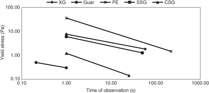
Figure 4.5 Time length of observation between the yield stress over short and long time scales of sage seed gum (SSG), cress seed gum (CSG), xanthan (XG), pectin (PE), and guar gum (GG).
4.2.4 Yield Stress
It is known that any material has a range of yield stress that depends on how they are measured [65]. Dynamic mechanical measurement is a valuable technique for the determination of the yield stress. The crossover stress (τ f at G′ = G″) is a good indicator of the yield stress when the structure ruptures and the flow behavior starts [66]. As the time frame of yield measurement is a key parameter, in our previous study [17], we obtained the yield stress under large deformation as a crossover point in the amplitude sweep test, which represented the yield stress over a short time scale (τ 0s ), and the yield stress under small deformation as a crossover point in the frequency sweep test (using the Cole–Davidson model) which occurred over a long time scale (τ 0l ). To obtain these parameters for the five mentioned hydrocolloids, strain sweep tests were conducted in the range of 0.01%–100% strain at a constant frequency of 1 Hz, and the frequency sweep measurements were performed within the LVE range over a frequency range of 0.01–100 Hz. The extent of shift (E s ) in the crossover points (the difference between the yield stresses over short and long time scales) was calculated as follows [17]:
where t 0l is the time of observation in the small deformation domain (the reciprocal of the frequency at the crossover point in the frequency sweep test), t 0s is the time of observation in the large deformation domain (the reciprocal of the frequency at the crossover point in the amplitude sweep test). As shown in Figure 4.5, PE showed the highest τ 0s value among all gums (35.76 Pa), while GG showed the lowest value of this parameter (0.30 Pa), and the other gums showed intermediate values. The yield stress is correlated with the strength of the coherent network structure throughout the volume of the material [26]. This result confirmed the greatest strength of PE and the weakest structure for GG. In addition, we determined the reciprocal of the frequency at the crossover points that represented the time at which each shear stress was observed. For all gum dispersions, the longer the observation period, the lower the yield stress measured, which confirmed that the yield stress is a time‐dependent property [65]. As strain sweep tests were performed at a constant frequency of 1 Hz for all gum systems, the time at which τ 0s occurred was the same for all gum dispersions. The highest time interval between τ 0l and τ 0s was obtained for PE, while the shortest distance was for GG. As the observation time of t 0l varied among different gums, one can conclude that PE demonstrated the longest‐lasting structure under small deformation. It is worth mentioning that in the time interval between t 0l and t 0s , the magnitudes of τ 0l and τ 0s of SSG were surprisingly close to those of XG (Figure 4.5). The distances between crossover points in the amplitude sweep and frequency sweep tests (E s ) were calculated in Cartesian space. Results showed that the extent of yield stress shift was the highest for PE (223.29), while this parameter was the lowest for GG (0.81). This behavior confirmed the highest rigidity of PE chains and the random coil conformation of GG.
4.3 Cluster Analysis
One of the most important unsupervised learning problems is clustering. This procedure is used for statistical data analysis in many fields, such as data mining. There are many clustering methods, such as the hierarchical clustering method. The agglomerative hierarchical method is a subclass of hierarchical clustering. Hierarchical clustering finds successive clusters using previously established clusters and merges them until the desired cluster structure is obtained [3]. PCA is a statistical method which uses sophisticated underlying mathematical principles to transform a number of possibly correlated variables into a smaller number of linearly uncorrelated variables called principal components [67]. Here, the similarity of the dynamic and transient shear rheological properties of two novel gums (SSG and CSG) with three commercialized biopolymers (GG, XG, and PE) were investigated by using the agglomerative hierarchical clustering technique (bottom‐up) and the PCA in a serial mode. In addition, the Euclidean distance, computed by finding the square of the distance between each variable, summing the squares, and finding the square root of that sum, was used as a distance measure [68]. The dynamic and transient shear rheological properties of five hydrocolloid dispersions were given by 52 parameters. As a high number of rheological parameters are introduced in this chapter, to use PCA for clustering, we applied a screening filter. Initially, the 52 parameters were classified into 5 categories with more than 65% similarity indexes in each group using agglomerative hierarchical clustering (Table 4.8). The first to fifth groups contained those variables associated with the elastic component, viscous component, viscoelastic component, plasticity, and conformation of hydrocolloids, respectively. Then, from each group, only one parameter, which represented one of the rheological aspects of matter (boldfaced parameter), was randomly selected for clustering. These five parameters were EANC concentration, the power‐law model's exponent of the double logarithmic plot of G″ against frequency (n″), the ratio of the power‐law model's intercepts of the double logarithmic plot of G′ and G″ against the frequency (k′/k″), plastic dissipation index (ϕ), and the slope of the double logarithmic scale plot of complex viscosity versus frequency (η* s ).
Table 4.8 Clustering of dynamic and transient rheological parameters of sage seed gum (SSG), cress seed gum (CSG), xanthan (XG), pectin (PE), and guar gum (GG) based on similarity index (S.I).
| A (S.I: 84.75) | B (S.I: 75.45) | C (S.I: 65.63) | D (S.I: 75.65) | E (S.I: 81.25) | |
| K′ (intercept of elastic modulus vs. frequency curve's power‐law model) | n″ (slope of viscous modulus vs. frequency curve's power‐law model) | J 1R (recovery due to the Kelvin–Voigt element) | a (speed of recovery phase) | Tan (δ) AF (slope of loss tangent after flow point) | η* s (slope of complex viscosity vs. frequency curve's power‐law model) |
| G′ LVE (elastic modulus at the LVE) | J max (maximum compliance) | J 1C (retarded compliance) | λ (time for reaching 1/e G 0 ) | (γ Fr ‐γ L ) / γ Fr % (Ductility) |
|
| Xc (degree of crosslinking) | J 2C * (contribution of the Maxwell dashpot to deformation at creep) | σ e (equilibrium stresses) | f * (crossover frequency) | ϕ (plastic dissipation index) | Extent of shear thinning |
| EANC (elastic active network chain concentration) |
|
A (intercept of complex modulus vs. frequency curve's power‐law model) | Tan (δ) LVE (loss tangent at the LVE) |
|
|
| υ (number density of crosslinks) | ξ (the distance between sequential crosslinking points) | 1/ k 2 (asymptotic value of the relaxed portion of the initial stress) |
|
G″ p /G″ LVE (extent of viscous modulus overshoot) | |
| J 0C % (instantaneous elastic compliance) | η 0 (Newtonian flow viscosity) | D b (Debora number) | Hλ min (relaxation strengths at short relaxation time) | — |
|
| J 0R % (initial recovery compliance) | K″ (intercept of G″ vs. frequency curve's power‐law model | 1/ k 1 (decay rate) | C p (critical relaxation time point) | — | β (extent of departure from Cox–Merz rule) |
| τ Fr (Fracture stress) | — | z (network extension) | K″/K′ (the ratio of power‐law model's intercepts of the double logarithmic plot of G′ and G″ against frequency) | — |
|
| λ ret (retardation time) |
|
||||
|
|
|||||
| α (shift factor) | |||||
| Extent of shear thickening | |||||
| b (order of recovery reaction) | |||||
| E s (extent of shift in crossover points) | |||||
Bolded parameters were randomly selected for clustering.
The Scree plot indicated that just two components can evaluate more than 90% of variances in the data (data not shown), and thus they were used for clustering analysis. According to Figure 4.6, the score plot for the first two components verified that from the rheological characteristics point of view (dynamic and transient shear rheological properties), CSG and SSG are more similar to GG and XG, respectively. The most effective rheological parameters in hydrocolloids clustering analysis were η* s , a conformation‐related parameter (0.58 coefficient for PC1) and ϕ,, which is related to the structure of hydrocolloids (0.55 coefficient for PC1), whereas n″ demonstrated the least influence (0.29 coefficient for PC1) on hydrocolloids clustering (data not shown).
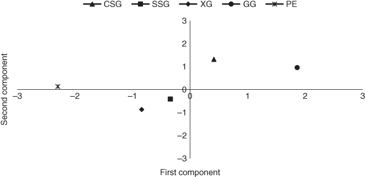
Figure 4.6 Distribution and correlation between the studied hydrocolloids in a vector space.
Table 4.9 Euclidean distance between sage seed gum (SSG), cress seed gum (CSG), xanthan (XG), pectin (PE), and guar gum (GG) in the vector space.
| Gum | XG | GG | PE | SSG | CSG |
| XG | 0.00 | 3.19b ± 0.10 | 1.80d ± 0.04 | 0.63c ± 0.06 | 2.49b ± 0.05 |
| GG | 3.19a ± 0.10 | 0.00 | 4.28a ± 0.06 | 2.42a ± 0.24 | 1.44d ± 0.07 |
| PE | 1.80c ± 0.04 | 4.28a ± 0.06 | 0.00 | 2.07ab ± 0.05 | 2.92a ± 0.06 |
| SSG | 0.63d ± 0.06 | 2.42c ± 0.24 | 2.07c ± 0.05 | 0.00 | 1.84c ± 0.07 |
| CSG | 2.49b ± 0.05 | 1.44d ± 0.07 | 2.92b ± 0.06 | 1.84b ± 0.07 | 0.00 |
a–d: Means followed by the same letters in the same column are not significantly different (P > 0.05).
Euclidean distances were calculated to quantitatively represent the similarity of different gums in the score plot as follows [68]:
where d ij is the Euclidean distance between a point X (X1, X2, etc.) and a point Y (Y1, Y2, etc.). According to Table 4.9, among the different commercialized hydrocolloids, SSG showed the lowest Euclidean distance with XG (0.63) and the highest distance with GG (2.42) and PE (2.07); in contrast, CSG showed the lowest Euclidean distance with GG (1.44) and the highest distance with XG (2.92). Besides, among galactomannans, SSG showed the highest similarity with PE with the lowest Euclidean distance magnitude. The variation in SSG and GG rheological behaviors could be related to the fact that although SSG and GG are galactomannans with approximately the same molecular weight (≈103 kDa for GG [6] and 4 × 10²–1.5 × 10³ kDa for SSG [ 10, 11]), SSG is a polyelectrolyte hydrocolloid whereas GG is a neutral polysaccharide. These physicochemical properties are reflected by the higher intrinsic viscosity of SSG (22.55 dl g−1 [10]) compared to that of GG (12.5 dl g−1 [6]). Also, it was expected that CSG, a polyelectrolyte galactomannan, would be similar to SSG rheologically, whereas it was similar to GG, which could be attributed to the lower molecular weight of CSG (540 kDa) compared with SSG. On the other hand, the polyelectrolyte nature of CSG could compensate for its negative effect of the lower molecular weight in comparison with GG, resulting in the greater similarity with GG, which is reflected in the similar intrinsic viscosity of CSG (13.3 dl g−1 [12]). The lowest Euclidean distance between SSG and XG may be attributed to the likeness of their conformation (rigid conformation of SSG and XG) [ 7, 10].
4.4 Conclusion and Future Trends
To better understand the elastic, viscous, and viscoelastic characters behavior of two novel hydrocolloids, SSG and CSG, and compare them with three generally used hydrocolloids, GG, XG, and PE, experiments based on unsteady state deformations, that is, oscillatory (in linear and nonlinear regions) and transient tests (in the linear region), were employed, and the similarity of these five hydrocolloids were investigated using the agglomerative hierarchical clustering technique and PCA. PE showed the highest storage modulus, complex modulus, limiting value of stress, fracture stress, and the slope of the loss tangent after the flow point and the lowest limiting value of strain, loss tangent, fracture strain, and reversible extensibility ahead of fracture among other hydrocolloids in the small deformation strain sweep test. XG, PE, and SSG showed G″ overshoot and were categorized as weak strain overshoot, whereas GG and CSG demonstrated strain thinning behavior. Only hydrocolloids which showed overshoot in G″ showed fracture properties. PE showed the highest, and GG, as well as CSG, showed the lowest values of spreadability, which were determined on the basis of the slope of the loss tangent after flow point stress (tan
δ
AF
). Qualitative investigation of LAOS flow revealed ideal viscoelastic behavior for XG, PE and SSG up to 1% and for GG and CSG up to 10% strain. These results were quantitatively confirmed by ![]() and
and ![]() for XG, PE, and SSG at 10% and 100% and GG at 100% strain. Using the Ewolt (2008) procedure, XG, PE and SSG showed intracycle strain‐stiffening behavior and GG showed strain‐softening behavior in their nonlinear strain domains. A full cycle study by Fourier series showed intercycle strain‐softening behavior for all the hydrocolloids at the 0.1%–10% and 0.1–100% strains, although XG, PE, and SSG showed greater first harmonic elastic modulus (
for XG, PE, and SSG at 10% and 100% and GG at 100% strain. Using the Ewolt (2008) procedure, XG, PE and SSG showed intracycle strain‐stiffening behavior and GG showed strain‐softening behavior in their nonlinear strain domains. A full cycle study by Fourier series showed intercycle strain‐softening behavior for all the hydrocolloids at the 0.1%–10% and 0.1–100% strains, although XG, PE, and SSG showed greater first harmonic elastic modulus (![]() ) reduction than did GG and CSG. In addition, except for GG, which did not show intercycle shear‐thickening behavior, the first harmonic viscous component of other gum dispersions showed different three‐stage dynamic viscosity versus shear rate responses with the Newtonian, shear‐thickening, and shear‐thinning behaviors in order. Among different parameters, intercycle nonlinearities were the most distinguishing parameters for different hydrocolloids. With an increase in strain, the plastic dissipation index (ϕ) values of SSG, XG, and PE approached the perfect plastic limit ϕ → 1, while it approached to the Newtonian fluid reference value (ϕ ≈ π/4 ≈ 0.785) for CSG and GG. There was great correlation between ϕ and tan
δ
AF
, which suggests the applicability of the ϕ parameter to determine the spreadability of materials. Over the frequency range 0.01–10 Hz, only GG showed the crossover frequency, while other hydrocolloids behaved as weak gels. The highest pseudoplasticity of PE in the dynamic shear rheological test in the small deformation mode is reflected by the highest η′ ratio reduction and the complex viscosity versus frequency slope (−0.867). Also, PE showed the highest gel strength, the highest number density of crosslinks, degree of crosslinking, EANC concentration, and the lowest distance between sequential crosslinking points among different hydrocolloids. Different relaxation spectra of hydrocolloids were investigated, and the results showed that the relaxation strengths at a short relaxation time, the extent of network strength, and the kinetic parameters of network strength change (C
p
and d(Hλ)/dλ) differed with respect to the gum types, which suggested different spatial arrangements. The most important contribution of the Maxwell spring to deformation, at creep (J
0C
≈ 30.40%) and recovery (
) reduction than did GG and CSG. In addition, except for GG, which did not show intercycle shear‐thickening behavior, the first harmonic viscous component of other gum dispersions showed different three‐stage dynamic viscosity versus shear rate responses with the Newtonian, shear‐thickening, and shear‐thinning behaviors in order. Among different parameters, intercycle nonlinearities were the most distinguishing parameters for different hydrocolloids. With an increase in strain, the plastic dissipation index (ϕ) values of SSG, XG, and PE approached the perfect plastic limit ϕ → 1, while it approached to the Newtonian fluid reference value (ϕ ≈ π/4 ≈ 0.785) for CSG and GG. There was great correlation between ϕ and tan
δ
AF
, which suggests the applicability of the ϕ parameter to determine the spreadability of materials. Over the frequency range 0.01–10 Hz, only GG showed the crossover frequency, while other hydrocolloids behaved as weak gels. The highest pseudoplasticity of PE in the dynamic shear rheological test in the small deformation mode is reflected by the highest η′ ratio reduction and the complex viscosity versus frequency slope (−0.867). Also, PE showed the highest gel strength, the highest number density of crosslinks, degree of crosslinking, EANC concentration, and the lowest distance between sequential crosslinking points among different hydrocolloids. Different relaxation spectra of hydrocolloids were investigated, and the results showed that the relaxation strengths at a short relaxation time, the extent of network strength, and the kinetic parameters of network strength change (C
p
and d(Hλ)/dλ) differed with respect to the gum types, which suggested different spatial arrangements. The most important contribution of the Maxwell spring to deformation, at creep (J
0C
≈ 30.40%) and recovery (![]() ), were those corresponding to PE, while GG showed the lowest value of these parameters. PE also had the highest recovery percentage during the creep/recovery test. The transient rheological behavior of hydrocolloids was investigated by using three well‐known viscoelastic models to fit the experimental data, where the Peleg model described the viscoelastic characteristics of all hydrocolloids appropriately, as compared to the Generalized Maxwell and Nussinovitch models. The Pleg model data suggested greater solid‐like behavior for PE and XG, whereas GG and CSG showed liquid‐like behavior in the stress relaxation test time scale. Except for GG, other hydrocolloids exhibited departure from the Cox–Merz rule, while PE showed the highest departure (85.35) followed by SSG (71.73). The yield stresses over a short time scale (τ
0s
) and over a long time scale (τ
0l
) were determined. PE showed the highest
τ
0s
value (35.76 Pa), while GG showed the lowest value of this parameter (0.30 Pa). In addition, the highest time interval between
τ
0l
and
τ
0s
was obtained for PE, while the shortest distance was for GG, which confirmed the highest rigidity of PE chains among the hydrocolloids. The hierarchical clustering technique with PCA indicated the highest similarity of SSG with XG and CSG with GG. In addition, the plastic dissipation index (ϕ) and the slope of the double logarithmic scale plot of complex viscosity versus frequency (η*
s
) were determined as the most effective rheological parameter in hydrocolloids clustering analysis.
), were those corresponding to PE, while GG showed the lowest value of these parameters. PE also had the highest recovery percentage during the creep/recovery test. The transient rheological behavior of hydrocolloids was investigated by using three well‐known viscoelastic models to fit the experimental data, where the Peleg model described the viscoelastic characteristics of all hydrocolloids appropriately, as compared to the Generalized Maxwell and Nussinovitch models. The Pleg model data suggested greater solid‐like behavior for PE and XG, whereas GG and CSG showed liquid‐like behavior in the stress relaxation test time scale. Except for GG, other hydrocolloids exhibited departure from the Cox–Merz rule, while PE showed the highest departure (85.35) followed by SSG (71.73). The yield stresses over a short time scale (τ
0s
) and over a long time scale (τ
0l
) were determined. PE showed the highest
τ
0s
value (35.76 Pa), while GG showed the lowest value of this parameter (0.30 Pa). In addition, the highest time interval between
τ
0l
and
τ
0s
was obtained for PE, while the shortest distance was for GG, which confirmed the highest rigidity of PE chains among the hydrocolloids. The hierarchical clustering technique with PCA indicated the highest similarity of SSG with XG and CSG with GG. In addition, the plastic dissipation index (ϕ) and the slope of the double logarithmic scale plot of complex viscosity versus frequency (η*
s
) were determined as the most effective rheological parameter in hydrocolloids clustering analysis.
These results can help the manufacturer decide on the final usage of SSG and CSG in various food formulations on the basis of the similarity of their oscillatory and transient rheological behaviors to the commercialized hydrocolloids, XG, GG, and PE. The approach presented in this chapter will help food scientists to gain a better insight into the structure–function relationship between hydrocolloids. In addition, the similarity of other physicochemical and structural properties of novel hydrocolloids could be investigated using the hierarchical clustering technique and PCA. Further work in this area is necessary for assessing the applicability and limitations of the emerging hydrocolloids in food and pharmaceutical systems.
References
- 1 Fox, P.F., Guinee, T.P., Cogan, T.M., and McSweeney, P.L.H. (2000). Cheese Yield, in Fundamentals of Cheese Science. Gaithersburg, MD: Aspen Publishers Inc.
- 2 Dea, I.C.M., Morris, E.R., Rees, D.A. et al. (1977). Associations of like and unlike polysaccharides: mechanism and specificity in galactomannans, interacting bacterial polysaccharides, and related systems. Carbohydrate Research 57: 249–272.
- 3 Azizpour, M., Mohebbi, M., Yolmeh, M. et al. (2017). Effects of different hydrocolloids on foaming properties of shrimp puree: a cluster analysis. Food Measurement and Characterization 11 (4): 1892–1898.
- 4 Casanovas, A., Hernandez, M.J., Martí‐Bonmati, E., and Dolz, M. (2010). Cluster classification of dysphagia‐oriented products considering flow, thixotropy and oscillatory testing. Food Hydrocolloids 25 (5): 851–859.
- 5 Serrano‐Megias, M. and Lopez‐Nicolas, J.M. (2006). Application of agglomerative hierarchical clustering to identify consumer tomato preferences: influence of physicochemical and sensory characteristics on consumer response. Journal of the Science of Food and Agriculture 86: 493–499.
- 6 Richardson, P.H., Willmer, J., and Foster, T.J. (1998). Dilute solution properties of guar and locust bean gum in sucrose solutions. Food Hydrocolloids 12: 339–348.
- 7 Higiro, J., Herald, T.J., and Alavi, S. (2006). Rheological study of xanthan and locust bean gum interaction in dilute solution. Food Research International 39: 165–175.
- 8 Sato, A.C.K., Oliveira, P.R., and Cunha, R.L. (2008). Rheology of mixed pectin solutions. Food Biophysics 3: 100–109.
- 9 Lopes da Silva, J.A. and Rao, M.A. (2006). Pectins: structure, functionality, and uses. In: Food Polysaccharides and Their Applications (ed. A.M. Stephen, G.O. Phillips and P.A. Williams), 65–94. Boca Raton: Taylor & Francis Group.
- 10 Razavi, S.M.A., Mohammadi Moghaddam, T., Emadzadeh, B., and Salehi, F. (2012). Dilute solution properties of wild sage (Salvia macrosiphon) seed gum. Food Hydrocolloids 29: 205–210.
- 11 Razavi, S.M.A., Cui, S.W., Guo, Q., and Ding, H. (2014). Some physicochemical properties of sage (Salvia macrosiphon) seed gum. Food Hydrocolloids 35: 453–462.
- 12 Karazhiyan, H., Razavi, S.M.A., Phillips, G.O. et al. (2009). Rheological properties of Lepidium sativum seed extract as a function of concentration, temperature and time. Food Hydrocolloids 23: 2062–2068.
- 13 Karazhiyan, H., Razavi, S.M.A., Phillips, G.O. et al. (2011). Physicochemical aspects of hydrocolloid extract from the seeds of Lepidium sativum. International Journal of Food Science and Technology 46: 1066–1072.
- 14 Behrouzian, F., Razavi, S.M.A., and Karazhiyan, H. (2013). The effect of pH, salts and sugars on the rheological properties of cress seed (Lepidium sativum) gum. International Journal of Food Science and Technology 48: 2506–2513.
- 15 Behrouzian, F., Razavi, S.M.A., and Karazhiyan, H. (2014). Intrinsic viscosity of cress (Lepidium sativum) seed gum: effect of salts and sugars. Food Hydrocolloids 35: 100–105.
- 16 Behrouzian, F., Razavi, S.M.A., and Phillips, G.O. (2014). Cress seed (Lepidium sativum) mucilage, an overview. Bioactive Carbohydrates and Dietary Fibre 3: 17–28.
- 17 Razavi, S.M.A., Alghooneh, A., and Behrouzian, F. (2018). Thermo‐rheology and thermodynamic analysis of binary biopolymer blend: a case study on sage seed gum‐xanthan gum blends. Food Hydrocolloids 77: 307–321.
- 18 Guo, Q., Cui, S.W., Wang, Q. et al. (2009). Microstructure and rheological properties of psyllium polysaccharide gel. Food Hydrocolloid 23: 1542–1547.
- 19 Heldman, D.R. and Lund, D.B. (eds.) (2007). Handbook of Food Engineering. New York: CRC Press.
- 20 Farahnaky, A., Askari, H., Majzoobi, M., and Mesbahi, G. (2010). The impact of concentration, temperature and pH on dynamic rheology of psyllium gels. Journal of Food Engineering 100: 294–301.
- 21 Sousa, A.M.M. and Gonçalves, M.P. (2015). The influence of locust bean gum on native and alkali‐modified agar gels. Food Hydrocolloids 44: 461–470.
- 22 Hyun, K., Kim, S.H., Ahn, K.H., and Lee, S.J. (2002). Large amplitude oscillatory shear as a way to classify the complex fluids. Journal of Non‐Newtonian Fluid Mechanics 107 (1–3): 51–65.
- 23 Hyun, K., Wilhelm, M., Klein, C.O. et al. (2011). A review of nonlinear oscillatory shear tests: analysis and application of large amplitude oscillatory shear (LAOS). Progress in Polymer Science 36 (12): 1697–1753.
- 24 Anvari, M. and Joyner, H.S. (Melito)(2017). Effect of formulation on structure‐function relationships of concentrated emulsions: rheological, tribological, and microstructural characterization. Food Hydrocolloids 72: 11–26.
- 25 Eissa, A.S., Bisram, S., and Khan, S.A. (2004). Polymerization and gelation of whey protein isolate at low pH using transglutaminase enzyme. Journal of Agricultural and Food Chemistry 52 (14): 4456–4464.
- 26 Sun, A. and Gunasekaran, S. (2009). Yield stress in foods: measurements and applications. International Journal of Food Properties 12 (1): 70–101.
- 27 Carmona, J.A., Ramirez, P., Calero, N., and Munoz, J. (2014). Large amplitude oscillatory shear of xanthan gum solutions. Effect of sodium chloride (NaCl) concentration. Journal of Food Engineering 126: 165–172.
- 28 Ewoldt, R.H., Hosoi, A.E., and Mckinley, G.H. (2008). New measures for characterizing nonlinear viscoelasticity in large amplitude oscillatory shear. Journal of Rheology 52 (6): 1427–1458.
- 29 Ewoldt, R.H., Winter, P., Maxey, J., and McKinley, G.H. (2010). Large amplitude oscillatory shear of pseudoplastic and elastoviscoplastic materials. Rheology Acta 49: 191–212.
- 30 Melito, H., Daubert, C., and Foegeding, E. (2013). Relating large amplitude oscillatory shear and food behavior: correlation of nonlinear viscoelastic, rheological, sensory and oral processing behavior of whey protein isolate/κ‐carrageenan gels. Food Process Engineering 36: 521–534.
- 31 Yaşar, K., Kahyaoglu, T., and Şahan, N. (2009). Dynamic rheological characterization of salep glucomannan/galactomannan based milk beverages. Food Hydrocolloids 23: 1305–1311.
- 32 Benchabane, A. and Bekkour, K. (2008). Rheological properties of carboxymethyl cellulose (CMC) solutions. Colloid Polymer Science 286: 1173–1180.
- 33 Razavi, S.M.A., Alghooneh, A., Behrouzian, F., and Cui, S.W. (2016). Investigation of the interaction between sage seed gum and guar gum: steady and dynamic shear rheology. Food Hydrocolloids 60: 67–76.
- 34 Morris, E.R., Cutler, A.N., Ross‐Murphy, S.B. et al. (1981). Concentration and shear rate dependence of viscosity in random coil polysaccharide solutions. Carbohydrate Polymer 1: 5–21.
- 35 Barnes, H.A. (2000). A Handbook of Elementary Rheology. Aberystwyth: University of Wales, Institute of Non‐Newtonian Fluid Mechanics.
- 36 Ross‐Murphy, S.B. (1988). Small deformation measurements. In: Food Structure‐Its Creation and Evaluation (ed. J.M.V. Blanshard and J.R. Mitchell). London: Butterworth Publishing Co.
- 37 Alghooneh, A., Razavi, S.M.A., and Behrouzian, F. (2016). Flow behavior, thixotropy and viscoelastic characterization of biopolymer blends: sage seed gum‐xanthan gum blends as a case study. Food Hydrocolloids 57 (21): 9609–9621.
- 38 Morris, E.R. (1990). Shear‐thinning of ‘random coil’ polysaccharides: characterisation by two parameters from a simple linear plot. Carbohydrate Polymer 13: 85–96.
- 39 Rafe, A. and Razavi, S.M.A. (2013). Dynamic viscoelastic study on the gelation of basil seed gum. International Journal of Science and Technology 48: 556–563.
- 40 Balaghi, S., Edelby, Y., and Senge, B. (2014). AIP Conference Proceedings 1593, The Polymer Processing Society Nuremberg, Germany.
- 41 Balk, M., Behl, M., Nöchel, U., and Lendlein, A. (2012). Shape‐memory hydrogels with switching segments based on oligo (ɛ‐pentadecalactone). Macromolecular Materials and Engineering 297: 1184–1192.
- 42 Gabriele, D.G., Migliori, M., Sanzo, R.D. et al. (2009). Characterization of dairy emulsions by NMR and rheological techniques. Food Hydrocolloids 23: 619–628.
- 43 Yoon, W.B. and Gunasekaran, S. (2007). Effect of temperature and concentration on rheological behavior of xanthan‐carob mixed gels. Biotechnology and Bioprocess Engineering 12 (3): 295–301.
- 44 Kontogiorgos, V. and Kasapis, S. (2016). Modeling and fundamental aspects of structural relaxation in high solid hydrocolloid systems. Food Hydrocolloids 68: 232–237.
- 45 Labropoulos, C.K., Rangarajan, S., Niesz, D.E., and Danforth, S.C. (2001). Dynamic rheology of agar cell based aqueous binders. Journal of the American Ceramic Society 84 (6): 1217–1224.
- 46 Ferry, J.D. (ed.) (1980). Viscoelastic Properties of Polymers. New York: Wiley.
- 47 Steffe, J.F. (ed.) (1996). Rheological Methods in Food Process Engineering. Michigan: Freeman Press.
- 48 Dolz, M., Hernandez, M.J., and Delegido, J. (2008). Creep and recovery experimental investigation of low oil content food emulsions. Food Hydrocolloids 22: 421–427.
- 49 Banville, V., Power, N., Pouliot, Y., and Britten, M. (2015). Relationship between baked‐cheese sensory properties and melted‐cheese physical characteristics. Journal of Texture Study 46: 321–334.
- 50 Petrocić, J., Fiśteś, A., Rakić, D. et al. (2015). Effect of defatted wheat germ content and its particle size on the rheological and textural properties of the cookie dough. Journal of Texture Study 46: 374–384.
- 51 Kuo, M.I., Wang, Y.C., and Gunasekaran, S. (2000). A viscoelasticity index for cheese meltability evaluation. Journal of Dairy Science 82: 412–417.
- 52 Kramer, A. and Szczesniak, A.S. (eds.) (1973). Texture Measurements of Foods: Psychophysical Fundamentals; Sensory, Mechanical, and Chemical Procedures and Their Interrelationships. Boston: D. Reidel Publishing, Co.
- 53 Razavi, S.M.A., Taheri, H., and Sunchez, R. (2013). Viscoelastic characterization of wild sage (Salvia macrosiphon) seed gum as a function of concentration. International Journal of Food Properties 16: 1604–1619.
- 54 Tang, J., Tung, M., and Zeng, A.Y. (1998). Characterization of gellan gels using stress relaxation. Journal of Food Engineering 38: 279–295.
- 55 Nussinovitch, A., Peleg, M., and Normand, M.D. (1989). A modified Maxwell and a nonexponential model for characterization of the stress relaxation of agar and alginate gels. Journal of Food Science 54 (4): 1013–1016.
- 56 Peleg, M. (1980). Linearization of relaxation and creep curves of solid biological materials. Journal of Rheology 24 (4): 451–463.
- 57 Peleg, M. and Normand, M.D. (1983). Comparison of two methods for stress relaxation data presentation of solid foods. Rheologica Acta 22: 108–113.
- 58 Mohsenin, N.N. (ed.) (1986). Physical Properties of Plant and Animal Materials. Structure, Physical Characteristics and Mechanical Properties. New York: Gordon and Breach Science Publishers, Inc.
- 59 Kajuna, S.T.A.R., Bilanski, W.K., and Mittal, G.S. (1998). Effect of ripening on the parameters of three stress relaxation models for banana and plantain. Applied Engineering in Agriculture 14 (1): 55–61.
- 60 Herrero, A.M., Heia, K., and Careche, M. (2004). Stress relaxation test for monitoring postmortem changes of ice‐stored cod (Gadus morua L.). Journal of Food Science 69 (4): 178–182.
- 61 Sozer, N. and Dalgic, A.C. (2007). Modelling of rheological characteristics of various spaghetti types. European Food Research and Technology 225: 183–190.
- 62 Li, S.‐P., Zhao, G., and Chen, H.‐Y. (2005). The relationship between steady shear viscosity and complex viscosity. Journal of Dispersion Science and Technology 26 (4): 415–419.
- 63 Cox, W.P. and Merz, E.H. (1958). Correlation of dynamic and steady flow viscosities. Journal of Polymer Science 28: 619–622.
- 64 Shatwell, K.P., Sutherland, I.W., Ross‐Murphy, S.B., and Dea, I.C.M. (1991). Influence of the acetyl substituent on the interaction of xanthan with plant polysaccharides – II. Xanthan‐guar gum systems. Carbohydrate Polymers 14: 115–130.
- 65 Cheng, D.C.‐H. (1986). Yield stress: a time‐dependent property and how to measure it. Rheologica Acta 25: 542–554.
- 66 Mysore, S.S. and Rudrapatnam, T.N. (2015). Modulation in the rheological behaviour of porcine pepsin treated guar galactomannan on admixture with κ–carrageenan. Carbohydrate Polymers 115: 253–259.
- 67 Lardy, F., Vennat, B., Pouget, M.P., and Pourrat, A. (2000). Functionalization of hydrocolloids: principal component analysis applied to the study of correlations between parameters describing the consistency of hydrogels. Drug Development and Industrial Pharmacy 26 (7): 715–721.
- 68 Madhulatha, T.S. (2012). An overview on clustering methods. IOSR Journal of Engineering 2 (4): 719–725.