
5.2
Directed Graphs
5.2.1 Introduction
Thus far in our discussion of graphs, we have not associated a “direction” with the edges of the graph. In many models, however, such as hyperlinks connecting webpages, traffic flow problems, we impose a direction on the edges. A directed graph (or digraph) is defined as a graph whose edges are “directed” from one vertex to another. We call these types of edges directed edges (or arcs). If a directed edge goes from vertex u to vertex v, then u is called the head (or source) and v is called the tail (or sink) of the edge, and v is said to be the direct successor of u and u is the direct predecessor of v. See Figure 5.30.
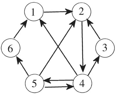
Figure 5.30 A directed graph with directed edges.
The applications of directed graphs range from transportation problems in which traffic flow is restricted to one direction and one‐way communication problems, to asymmetric social interactions, athletic tournaments, and even the World‐Wide Web. Before talking about applications, however, we introduce the concept of the adjacency matrix of a directed graph.
For example, the adjacency matrix for the digraph in Figure 5.30 is

5.2.2 Tournament Graphs (Dominance Graphs)
A tournament graph (or dominant graph) is a directed graph where every pair of vertices is joined by exactly one directed edge. In other words, for every pair of vertices u and v, there is a directed edge from u to v or a directed edge from v to u. Figure 5.31 shows a tournament graph with five vertices.
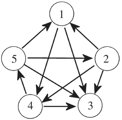
Figure 5.31 Tournament graph with five vertices.
Tournament graphs are aptly named since they model round‐robin tournaments in tennis, baseball, and so on, where every team plays every other team exactly once, where we assume no ties.
The number of directed edges “leaving” a vertex u is called the out‐degree of the vertex and denoted by od(u). In the directed graph in Figure 5.31, we have od(5) = 3, od(1) = 2. If the vertices of a directed graph represent athletic teams, a directed edge from vertex u to vertex v means team u beats team v and the out‐degree of u represents the number of wins for team u. On the other hand, the number of directed edges arriving at a vertex v is called in‐degree of v and denoted by id(v). In the graph in Figure 5.31, we have id(5) = 1, id(1) = 2. In connection with athletic tournaments, the in‐degree of vertex v represents the number of losses for team v.
Tournament graphs are even used by sociologists, who call them dominance graphs, and are used to model social interactions.
5.2.3 Dominance Graphs in Social Networking
Many social situations involve people or groups of people (countries, cultures, universities, and so on) in which some individuals or groups “dominates” others. The word “dominate” can refer to a wide variety of dominance: cultural, physical, political, economic, and so on. Nowadays, online social networking services such as Facebook, Twitter, LinkedIn, and so on, bring people together and offer interesting dynamics between individuals.
Suppose a sociologist wishes to study dominance patterns in a close‐knit group of college women. The group consists of five students: Amy (A), Betty (B), Carol (C), Denise (D), and Elaine (E). The sociologist begins by conducting interviews with each pair to determine their pair‐wise dominance.1 If it has been determined that person A dominates person B by some metric, we denote this by writing A → B. (We assume in this simple model that for each pair of students, one person dominates the other.) After conducting the interviews, the sociologist draws the dominance graph that represents pair‐wise dominations of the entire group, which is shown in Figure 5.32. Note that Amy dominates Betty and that Denise dominates Carol.

Figure 5.32 Dominance graph.
The adjacency matrix for the dominance graph is drawn in Figure 5.33.

Figure 5.33 Adjacency matrix.
The number of one's in each row is the out‐degree of the row vertex and represents the number of first‐stage dominances of that individual. Note that Amy and Denise each have a “score” of three, Carol and Elaine each have a score of two, and Betty has a score of zero. In other words, Amy and Denise are tied after the first round.
The goal is to find the group leader.2 If one person dominates more people than all others in the first round, then that person is declared group leader. However, if two or more people tie in the first round, we resort to second‐stage dominances. In our example, we have a tie between Amy and Denise, so we move on to the second round.
To understand second‐stage dominances, note that Elaine dominates Denise and Denise dominates Amy. Hence, we say that Elaine has a second‐stage dominance over Amy and denote this by Elaine → Denise → Amy. To find the number of second‐stage dominances, we find the square3 of the adjacency matrix M2, which is given in Figure 5.34.
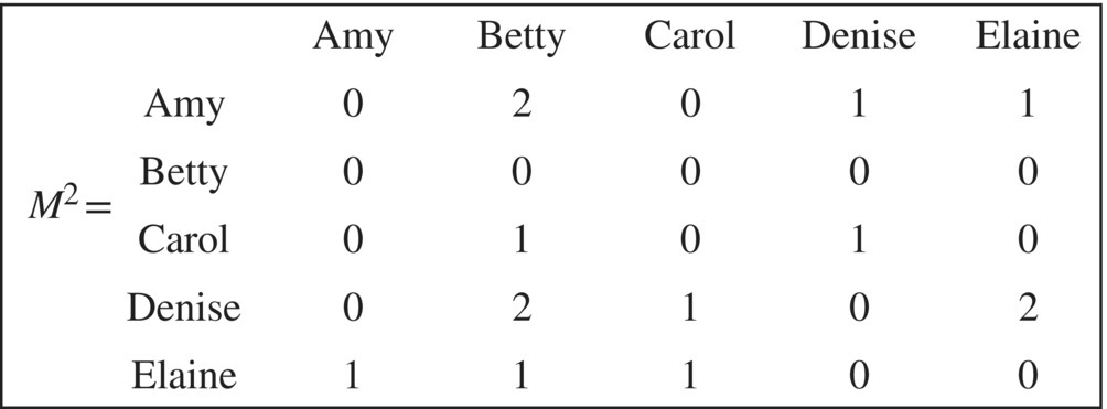
Figure 5.34 Second order dominances.
To interpret M2, note that Amy → Elaine → Denise, which is the only second‐stage dominance of Amy over Denise. This fact is indicated by the one in row Amy, column Denise of M2. Amy has 2 second‐stage dominances over Betty (Amy → Carol → Betty) and (Amy → Elaine → Betty), indicated with a two in row Amy, column Betty of M2. In other words, the elements of M2 give the second‐order dominances of row members over column members. From M2 we see that Denise has a total of 5 second‐state dominances (sum of the numbers in row Denise) while Amy has four (sum of the numbers in row Amy). Thus, we declare Denise the second‐stage group leader.4
We could continue by finding third‐order dominances, but we stop here and find the sum of the matrices M + M2, whose elements give the total number of first‐stage and second‐stage dominances of each individual shown in Figure 5.35.
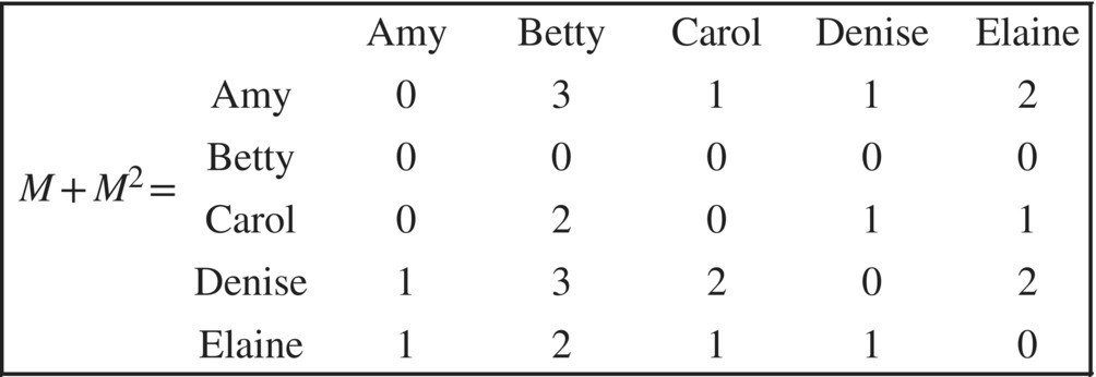
Figure 5.35 First and second order dominances.
Here, Amy has a total of 7 first‐ and second‐stage dominances over the members in the group while Denise has 8, so we call Denise the leader of the group.
It is interesting that a group leader in the social network depends on the out‐degrees of the vertices, whereas for ranking webpages on the Internet, one focuses on the in‐degrees or the number of links pointing to a webpage.
5.2.4 PageRank System
Google's search engine models the Internet as a directed graph where vertices are websites and the edges are links between websites. The strategy behind Google's PageRank system is based on counting the number and quality of links to a website as a way to measure the importance of the site. Consider the tiny Internet of four websites as drawn in Figure 5.36 with several individuals online. The numbers on the edges of the digraph estimate the probability that an individual in the column website will move to the row website.
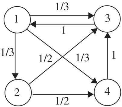
Figure 5.36 Web graph of a small internet.
The digraph in Figure 5.35 gives rise to the transition matrix in Figure 5.37.

Figure 5.37 Transition matrix.
Note that an individual at website one will probably move to websites two, three, or four with equal probabilities of 1/3, whereas an individual at website three will probably move to website one.
Initially, we assume the fraction of individuals at each website is 0.25, which we represent by the PageRanks of the four sites:
The idea is to simulate the movement of online individuals, using the transition matrix, and estimate the fraction of individuals frequenting each website after a period of time. To determine this fraction after one “click of the mouse,” we compute the product of the transition matrix with the initial PageRank distribution, or
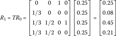
This new PageRank tells us, probabilistically speaking, that 25% of online individuals will favor website one, 8% website two, 45% website three, and 21% favor website four. These fractions come from multiplying the fraction of individuals that prefer a given website times the probability people at that website will move to the next website. The calculations that yield the values in R1 are
- fraction at website 1 =(1)(0.25) = 0.25
- fraction at website 2 =(1/3)(0.25) = 0.08
- fraction at website 3 =(1/3)(0.25) + (1/2)(0.25) + (1)(0.25) = 0.45
- fraction at website 4 =(1/3)(0.25) + (1/2)(0.25) = 0.21
We now continue this process again and again, finding
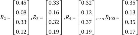
which in the long run we interpret that 35% of individuals will be on webpage 1, 13% on webpage 2, 35% on webpage 3, and 17% on webpage 4. This ordering gives search engines a way of measuring the popularity and importance of website pages.
5.2.5 Dynamic Programming
Many applications of directed graphs relate to the movement of objects – be it cars, trucks, airplanes, or even Internet packets from one location to another, and the objects being moved involve costs. Figure 5.38 shows a directed graph which represents a collection of possible paths from the “start” to the “end” with numbers on the edges representing the distance of traversing the edge. The problem is to find the path that minimizes the total distance of going from the start to the end.

Figure 5.38 Minimum path problem.
Although a quick examination of this small graph will convince you the minimum path is 1 − 3 − 4 − 7 − 9, resulting in a minimum distance of 13, for larger graphs with maybe 1000 nodes a visual inspection of the graph would probably provide no useful information about the shortest path.
To solve this problem, we use a powerful technique called dynamic programming, introduced by Richard Bellman in the 1950s. The general philosophy of the technique is to subdivide complex problems into smaller parts, solve the component parts and use these results to solve the larger problem.
In the current problem, the strategy is to work backwards, from the end node to the starting node. We begin by introducing the quantity
In the graph in Figure 5.38, we have s9 = 0, s7 = 4, s6 = 9, s8 = 10. Our goal is to find s1 We now let
which means d12 = 3, d46 = 5, and so on. Hence, dij + sj= distance from vertex i to vertex j plus the smallest distance from j to the end.
To find the shortest distance si from vertex i to the end, we compute the minimum of
taken over all vertices j connected to vertex i. For example, to find the shortest distance s4 from vertex i = 4 to the end, we find the minimum of the following four distances
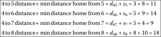
Taking the minimum of these subproblems, the shortest distance from vertex four to the end vertex is s4 = 9. We continue this process, moving backward in the graph and finding the minimum distances s8, s7, … , s1 from each vertex, although not necessarily descending in perfect order. We now advise the reader to get out pencil and paper compute the minimum distance to the end from each vertex, eventually finding s1, the shortest distance from the starting vertex to the final vertex. The computations in Table 5.1 show the shortest distant si to the end from every vertex i in the graph.
Table 5.1 Finding minimum distance to the end.
| Vertex | s i = minimum path to end from vertex i | Path |
| 9 | s9 = 0 | |
| 8 | s8 = d89 + s9 = 10 + 0 = 10 | 8 → 9 |
| 7 | s7 = d79 + s9 = 4 + 0 = 4 | 7 → 9 |
| 6 | 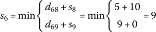 |
6 → 9 |
| 5 | s5 = d57 + s7 = 4 + 4 = 8 | 5 → 7 |
| 4 | 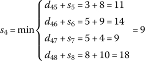 |
4 → 7 |
| 3 |  |
3 → 4 |
| 2 | 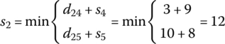 |
2 → 4 |
| 1 |  |
1 → 3 |
Hence, the minimum distance from vertex 1 to vertex 9 is 13 and retracing the path from start to end we find path that gives the shortest distance is 1 → 3 → 4 → 7 → 9.
Problems
- Problems 1–6 find the adjacency matrix M of the given digraph. Then compute M2 and M + M2 and verify that the elements of these matrices agree with the number of dominations in the graphs.

Figure 5.39 Find the adjacency matrix. -
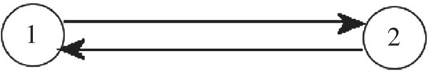
Figure 5.40 Find the adjacency matrix. -

Figure 5.41 Find the adjacency matrix. -

Figure 5.42 Find the adjacency matrix. -
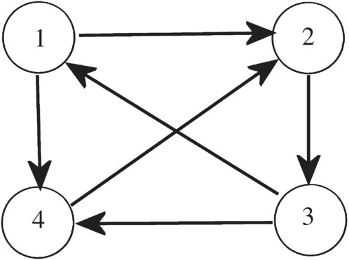
Figure 5.43 Find the adjacency matrix. -
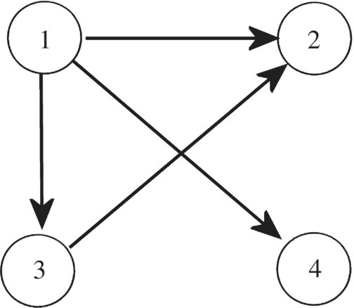
Figure 5.44 Find the adjacency matrix. - Group Dominance
The graph shown in Figure 5.45 shows the dominance of a group of four classmates: Amy, Betty, Charlie, and Denise.
- Construct the adjacency matrix M for this graph.
- Is there a first‐stage dominance leader?
- Compute M2 and interpret its elements.
- Who is the group leader?
- Which person is dominated by the most other people?

Figure 5.45 Group dominance.
- Round‐Robin Tournaments
The graph in Figure 5.46 shows the results of a round‐robin tournament for five baseball teams.
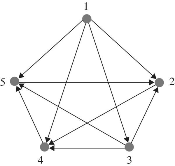
Figure 5.46 Round robin tournament.
Round‐robin tournament graph
- Construct the adjacency matrix M for this graph.
- Is there a consensus leader for the group?
- Compute M2 and interpret its elements.
- Which team is the conference winner?
- Landau's Theorem
A theorem by Landau states that if some vertex u in a dominance graph has a larger out‐degree than all other vertices, then either u dominates all other vertices v, or if it does not dominate a given vertex v, then u dominates a third vertex w which in turn dominates v. What does the theorem say in the language of round‐robin tournaments? Verify this theorem for the dominance graphs in Problems 1–6.
- Landau's Theorem in the Yankee Conference
Suppose the football teams in the Yankee Conference play every other team exactly once during the season. At the end of the season, Maine has won more games than any other team. However, Maine lost to Vermont. What does Landau's theorem say in the language of the Yankee Conference?
- Dynamic Programming
Use dynamic programming to find the shortest way to accomplish the project in Figure 5.47.
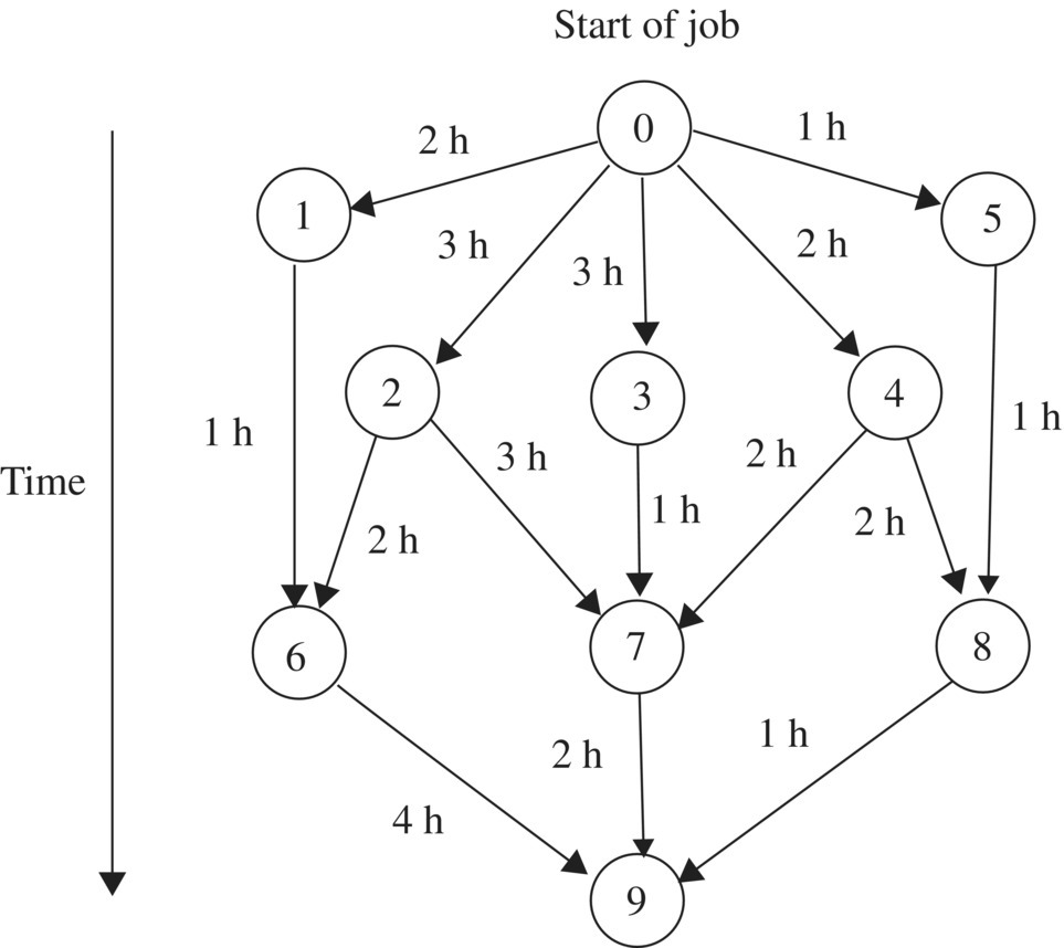
Figure 5.47 Shortest time problem.
- Ranking Webpages
The dominance graph in Figure 5.48 illustrates a tiny Internet of four webpages where the vertices represent the webpages and the directed edges represent links from one webpage to another. Rank the webpages from first to last. Note that node 1 moves to nodes 2, 3, and 4, each with probability 1/3, whereas node 2 moves to nodes 3 and 4, each with probability 1/2.
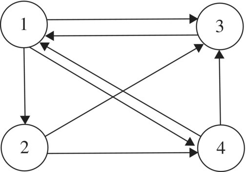
Figure 5.48 Ranking webpages.
- Game Time on a Directed Graph
Sixteen objects are placed on a table. At each play of the game, each player selects either 1, 2, 3, or 4 objects from the pile. The players alternate turns and the person who takes the last object (or objects) from the table wins. Draw a directed graph of 17 vertices labeled from 0 to 16 illustrating the number of objects on the table and directed edges between vertices that give the best possible move at each vertex. The player who starts the game will always win if the right strategy is used. Find the different paths through the graph from vertex 16 to vertex 0 what will ensure the first player wins. What is the strategy?
- Internet Research
There is a wealth of information related to topics introduced in this section just waiting for curious minds. Try aiming your favorite search engine toward applications of directed graphs, Google's PageRank system, directed graphs in social rankings, and directed graphs in athletic rankings.