
CHAPTER 5
Advanced Deep Learning
In the previous chapter, we started building deep neural network models for analyzing images using Keras and TensorFlow. Now in this chapter we will start building models that extract complex visual patterns. We will go beyond the MLP into Convolutional Neural Networks (CNN) and show how they are much more effective in building deep models specifically for image analysis. We will use different data in this chapter—a fashion items images dataset. Hopefully it will be interesting and you can try on some of your own image data.
The Rise of Deep Learning Models
In the previous chapter, we saw one type of neural network called the multi‐layered perceptron (MLP). These were the most common types of neural network used in the 1990s. However, these networks have many limitations.
MLP is good for a limited set of features, such as the less than one thousand in our example. As the number of features increases, since all neurons in dense layers are connected to all neurons in the next layer, the weights become very large. This makes the model difficult to train and requires a lot of processing power. As we add more layers with neurons in MLP, we don't see the effect of these layers much in the accuracy. So, adding more dense layers adds to complexity and training time, but doesn't really provide much benefit.
Also, we saw in our example that a 28×28 image was changed into a one‐dimensional 784‐element vector. This became the input layer for our network. However, when we flatten the two‐dimensional layer, we lose many spatial relationships that the image carries. The two‐dimensional structure carries relationships between pixels that help us understand the pattern the image contains. These are lost when we just flatten and give the inputs to an MLP.
We saw that in order to send unstructured data like images through an MLP, a large amount of feature extraction was needed to get meaningful results. This may be in the form of resizing large images to a smaller size, making images grayscale to reduce dimension, thresholding images to remove noise, etc. Many of these techniques fall in the domain of computer vision, which is basically a method to extract knowledge from images stored digitally as pixel arrays. Similar approaches were needed while handling other types of data like audio or text. In short, to get effective results from MLPs, a lot of feature extraction was needed. This process is known as feature engineering.
For a while in the 1990s, neural networks started going out of favor due to these limitations. However, in the early 2010s new discoveries in the types of network layers and architectures of neural networks started overcoming these limitations. Around the same time, there were tremendous improvements in processing power with advanced hardware like GPUs that could do thousands of linear Algebra calculations in parallel. This caused the advent of a new discipline under the Machine Learning umbrella known as Deep Learning (DL). DL is technically a sub‐branch of ML and more specifically a type of supervised learning. However, DL has been able show some amazing results in many challenging problems like image classification, natural language processing, speech recognition, voice synthesis, and many more. This makes DL a discipline of great importance and it is fast becoming the face of Artificial Intelligence. Again, since at its heart, DL is still a supervised learning method, all the concepts we learned about earlier, such as bias, variance, underfitting, and overfitting, are still valid for DL models.
New Kinds of Network Layers
One of the major improvements that DL introduces is new types of layers that help to build special types of models. These models work well on specific types of unstructured data like images or text. As we saw earlier, dense layers greatly increase the number of weights that need to be stored in the model. Also, they don't capture spatial relationships of the data, which are prominent in images. Let's look at how DL provides specialized layers and network architectures to help in image analysis. These types of networks are specialized neural networks known as Convolutional Neural Networks (CNNs). CNNs have been universally accepted as the best models available today for analyzing images and extracting knowledge from them. Let's look at these in detail.
Convolution Layer
As the name suggests, the major improvement in CNNs over regular MLP networks is the introduction of a new layer of neurons called a convolution layer. This layer specializes in extracting spatial patterns in pixel arrays. Let's look at this layer in detail.
Convolution is the operation of running a smaller matrix (known as a filter) over a larger data or signal matrix. At each run we do an element‐wise multiplication of the two matrix elements and then add them. Consider convolution with the visual example shown in Figure 5.1.

Figure 5.1: Simple convolution filter to extract horizontal lines
Our test image is a binary image with one horizontal and one vertical line, making a cross. This image is made up of 1s and 0s, indicating white and black pixels, respectively. We see the array representation of this image—with nine rows and nine columns. We choose a particular convolution filter (also called a kernel) of shape 2×2 and move it across the image. At each move we do element‐wise multiplication and add the results. We get a new array that is of size 8×8. We see something interesting when we represent this new array as an image. We see the new convolved image only has the horizontal line highlighted. We were able to extract the pattern of horizontal lines from this image.
Now let's use a different filter and see what we can get. See Figure 5.2.

Figure 5.2: Simple convolution filter to extract vertical lines
Our next filter can detect vertical lines. It looks for particular patterns in the two‐dimensional image and the result is an array with only the vertical lines with non‐zero values.
If we take the two‐dimensional image array as a layer in our neural network, applying this convolution filter will give us a new layer with only the vertical neurons activated. This is the concept of the convolution layer in CNNs.
The convolution layer is a three‐dimensional layer. Two of its dimensions are the width and height of the input image. The third dimension is the number of filters we want our network to learn. As our network consumes the data points (training images in this case), it learns which features are of interest and starts learning those filters. Maybe the images you feed have many horizontal lines—then it will start learning the horizontal line filter we saw earlier. Typically, we use higher‐order filters like 3×3, 5×5, or 7×7. The 2×2 filter was just an example to show how convolution works.
We saw in the previous examples that after applying a filter, the size of the image reduced a little bit. We went from a 9×9 image to an 8×8 one. This is a straightforward calculation. Basically:
New Image Dimension = Image Dimension – (filter size – 1) This applies both to the width and height of the image. We normally use square filters—so the filter size is the same for both—three in 3×3 and five in 5×5. Many times, you don't want the convolution layer to change dimensions of your image. In that case, you add padding. With padding, the convolution operation basically returns an image of the same size as the input image, but with the patterns extracted by the convolution layer.
There are a few other layers of interest in CNNs and deep networks in general. We will go through a brief description and then explore them better with an example.
Pooling Layer
The key difference between MLP and CNN is that CNN works with two‐dimensional image arrays and tries to extract spatial patterns using convolution layers. However, we need layers that can also reduce the dimension of images so we can improve upon the processing time. This is done using the pooling layer. All it does is down‐sample the image based on a summary statistic like average or maximum. MaxPooling2D is a popular pooling layer that uses a pooling window like 2×2 or 4×4. It takes the maximum of the values in the window and assigns that to new image. It reduces the size of the image array by the amount of the window selected. For example, a 2×2 window will down‐sample a 100×100 image to 50×50.
We have already seen a flatten layer earlier that converts the two‐dimensional array into a single‐dimensional vector. The major difference in a CNN is that we use the flatten layer at the end of network after the convolution layers have extracted relevant patterns.
Now before we code an example, let's look at two special types of layers.
Dropout Layer
Many times, CNNs tend to overfit on the training data, with certain neurons always looking for fixed patterns in training data. One way to prevent this overfitting and increase the bias of the network is to use a special type of layer known as a dropout. A dropout layer basically drops a fixed percentage of neurons from our network at random during each training iteration or batch. So, a dropout of 0.3 means we randomly take 30% of neurons entering this layer and make their value zero. Now these neurons no longer play a role in learning. This way the network does not get a chance to overfit on training data because at any batch iteration any random neurons may be zero.
Batch Normalization Layer
We saw in the MLP example on the MNIST data earlier that we got training and test datasets with pixel intensity values between 0 and 255. We normalized these data points by dividing by 255, thus making the values between 0 and 1. This helps speed up the training process and our network converges faster. Another very popular way of speeding up training is to use a special layer known as a batch normalization layer. This layer basically does the normalization of data flowing through the network but at any layer. So instead of only normalizing input data, we also normalize data between layers so the network learns faster and we get good results.
Building a Deep Network for Classifying Fashion Images
All right, now let's see all this in action. We will take the earlier MNIST example and modify it to use CNN instead of MLP.
First, just as we saw earlier, let's load the data and look at the dataset. For this example, we will use a new dataset also provided by Keras—the fashion items dataset (see Figure 5.3). This dataset also has 28×28 grayscale training and test images like MNIST. These images are of fashion items rather than digits. Also, we will use a labels array to define labels for each item. See Listing 5.1.

Figure 5.3: Samples from fashion images dataset
Now we will build a CNN using some of the layers we saw earlier. The concept of CNN is first to keep the image input in two dimensions and apply convolution and pooling. Then we flatten the data and build a dense layer to map to 10 outputs with a Softmax layer. The network's structure is shown in Figure 5.4.

Figure 5.4: Simplified architecture of our CNN model
Let's code this network. First, we do some preprocessing on the data. We convert the integer Y values to one‐hot encoded array of 0s with only the prediction column with value 1. Next, we divide the values by 255 to normalize the data between 0 and 1. Finally, we use the numpy expand_dims function to change the array (or Tensor) from (num_samples, 28, 28) to (num_samples, 28, 28, 1)—one dimension. This does not change the data but reshapes the matrix to make it easier to feed the CNN. See Listing 5.2.
Now let's build the network. As shown in Figure 5.4, we will use a convolution layer with 32 filters and max pooling with a 4×4 pool size in 2D. We will then flatten and apply a dense layer of size 10 to indicate the predictions. See Listing 5.3.
Here are the results:
_________________________________________________________________Layer (type) Output Shape Param #=================================================================conv2d_18 (Conv2D) (None, 28, 28, 32) 320_________________________________________________________________max_pooling2d_17 (MaxPooling (None, 7, 7, 32) 0_________________________________________________________________flatten_11 (Flatten) (None, 1568) 0_________________________________________________________________dense_12 (Dense) (None, 10) 15690=================================================================Total params: 16,010Trainable params: 16,010Non‐trainable params: 0
Let's compare the CNN model to the MLP we built earlier. One thing you notice immediately is that the total trainable parameters or weights in the CNN is 16,010, while the ones in the MLP were 407,050. That is the advantage of using convolution and pooling layers. They capture patterns but use way fewer weights. This is because the convolution layer reuses weights by having the same filter convolve over the previous layer again and again.
This makes the CNN model much lighter to load and faster to train and predict. Now let's train our model; see Listing 5.4.
Since this is a more complex dataset than MNIST, we get a lower accuracy in the first epoch. You will get similar accuracy values using an MLP, but with a huge model size. As you increase the epochs, you will get more improvements in accuracy. We will plot the accuracy and loss over time with epochs. Let's run for 20 epochs and see how the loss and accuracy vary. See Listing 5.5.
Here are the results:
Epoch 1/2060000/60000 [==============================] ‐ 19s 314us/step ‐ loss: 0.3605 ‐ acc: 0.8722Epoch 2/2060000/60000 [==============================] ‐ 17s 278us/step ‐ loss: 0.3234 ‐ acc: 0.8851Epoch 3/2060000/60000 [==============================] ‐ 15s 248us/step ‐ loss: 0.3031 ‐ acc: 0.8933Epoch 4/2060000/60000 [==============================] ‐ 15s 250us/step ‐ loss: 0.2893 ‐ acc: 0.8971Epoch 5/2060000/60000 [==============================] ‐ 15s 251us/step ‐ loss: 0.2785 ‐ acc: 0.9007Epoch 6/2060000/60000 [==============================] ‐ 15s 256us/step ‐ loss: 0.2679 ‐ acc: 0.9052Epoch 7/2060000/60000 [==============================] ‐ 16s 260us/step ‐ loss: 0.2608 ‐ acc: 0.9077Epoch 8/2060000/60000 [==============================] ‐ 15s 247us/step ‐ loss: 0.2536 ‐ acc: 0.9095Epoch 9/2060000/60000 [==============================] ‐ 15s 257us/step ‐ loss: 0.2468 ‐ acc: 0.9123Epoch 10/2060000/60000 [==============================] ‐ 15s 247us/step ‐ loss: 0.2420 ‐ acc: 0.9133Epoch 11/2060000/60000 [==============================] ‐ 15s 248us/step ‐ loss: 0.2354 ‐ acc: 0.9159Epoch 12/2060000/60000 [==============================] ‐ 15s 246us/step ‐ loss: 0.2320 ‐ acc: 0.9165Epoch 13/2060000/60000 [==============================] ‐ 15s 248us/step ‐ loss: 0.2274 ‐ acc: 0.9181Epoch 14/2060000/60000 [==============================] ‐ 15s 248us/step ‐ loss: 0.2227 ‐ acc: 0.9200Epoch 15/2060000/60000 [==============================] ‐ 15s 250us/step ‐ loss: 0.2197 ‐ acc: 0.9213Epoch 16/2060000/60000 [==============================] ‐ 15s 247us/step ‐ loss: 0.2158 ‐ acc: 0.9236Epoch 17/2060000/60000 [==============================] ‐ 15s 251us/step ‐ loss: 0.2125 ‐ acc: 0.9222Epoch 18/2060000/60000 [==============================] ‐ 15s 247us/step ‐ loss: 0.2099 ‐ acc: 0.9254Epoch 19/2060000/60000 [==============================] ‐ 15s 244us/step ‐ loss: 0.2071 ‐ acc: 0.9252Epoch 20/2060000/60000 [==============================] ‐ 15s 244us/step ‐ loss: 0.2038 ‐ acc: 0.926710000/10000 [==============================] ‐ 1s 115us/step
Now we will take the learning history data stored in the history variable and plot it. See Listing 5.6.
Let's look at the plot of accuracy and loss over the epochs in Figure 5.5 below.

Figure 5.5: Model accuracy increases and loss decreases over the epochs
We see the model accuracy increase gradually over epochs and loss reduces. We can try different model architectures and hyper‐parameters to see what gives us the best results on our dataset. This is mostly done by trial and error, but many veteran data scientists have their favorite methods of tuning hyper‐parameters to get the best results. These hyper‐parameters may be number of layers, type of layers, number of neurons in each layer, loss function, optimizer used, etc. Let's look at some common ways data scientists tune their models by adjusting architectures and hyper‐parameters.
CNN Architectures and Hyper‐Parameters
CNNs can easily get very complex with many layers of neurons and different parameters. There are a few common practices data scientists use that can help better tune hyper‐parameters and save a lot of time. Because the models are complex and need large volumes of data to train, usually these take a lot of time and need specialized expensive hardware like GPUs to train.
First, we have to decide on the architecture of the neural network. This includes how many layers, what type of layers, and how many neurons in each layer. Earlier we saw a very simple network with one convolutional, one pooling, and one dense layer. However, that won't work when we have millions of images to classify into thousands of categories (yes people have tried that!). There are a few popular deep network architectures for CNN that have shown very good results on image classification problems. But how do we compare these? We need a standard image dataset to do so.
That's where ImageNet comes into the picture. This is a standardized image dataset with 14 million training images that are hand‐annotated into about 20 thousand categories. There are also a few thousand separate validation and testing datasets for evaluating your image classification models. Interestingly, ImageNet was a community effort lead by Fei Fei Li who is (as of 2018) the Chief Scientist working at Google.
Now with ImageNet, data scientists across the world can come up with innovative deep network architectures and evaluate on a common and standard dataset. When you present your next Deep Learning model architecture, you confidently say you tested it on ImageNet with 70% accuracy and everyone will know what that is. There is also an annual ImageNet Large Scale Visual Recognition Challenge (ILSVRC) organized every year where computer vision and AI scientists from universities and companies across the world compete on ImageNet. Pretty awesome stuff!
Figure 5.6 shows the common standard image dataset. Extremely smart data scientists around the world have been developing innovative deep network architectures to solve the image recognition problem. All these architectures have been published in the public domain—especially those that have participated in and won the ILSVRC competition over the years.

Figure 5.6: ImageNet categorized images (Source: Image‐Net.org)
Some of these popular architectures are AlexNet, VGG, ResNet, Inception, and more. I will provide some papers in the “References” section at the end of the book describing each of these in detail for those interested. Also, keep in mind that this is an area of active and ongoing research. So, as you are reading this book there may be a super‐smart data scientist somewhere in the world coming up with the next great architecture that will out‐perform all others.
Typically, it is recommended to start with one of the proven architectures and fine‐tune it for your requirements. The good news is that Keras comes packaged with most of these popular architectures. You can start with one of these and use it to train on your dataset. Moreover, Keras also gives you these models pretrained on the most popular open data source for image classification—ImageNet!
You will typically start with a good, proven model architecture like VGG or ResNet or Inception, then tune the hyper‐parameters to solve the particular problem you are dealing with. A couple other hyper‐parameters we may think of tuning are the loss function and the type of optimizer to be used. Typically, cross‐entropy or log loss is a popular loss function for classification problems. Cross‐entropy loss could be binary or categorical depending on if the problem is to classify between two classes (binary) or multiple classes (categorical). We have seen the standard batch, stochastic, and mini‐batch gradient descent optimizers. We may want to make the learning process faster by using different learning rates that work with these optimizers. Also, specialized optimizers like stochastic gradient descent (SGD) with Momentum, RMSProp, and Adam (which we used in the last example) may show better results. SGD with momentum tries to push the weight values (applies momentum) in the direction of the minima (optimal weights with minimum loss value). RMSProp tends to remove oscillations around certain weights while approaching the minima. Typically, Adam is more popular since it captures the effects of both Momentum and RMSProp. You may have to do lot of trial and error to arrive at the best optimizer for your problem.
The learning rate decides how big a step you take while modifying weights to approach the minima. A bigger learning rate may have you oscillating around the minima while a smaller rate may have you take a long time to reach it. Again, a lot of trial and error involved.
Making Predictions Using a Pretrained VGG Model
We will talk about a relatively simpler Deep Model—VGGNet by VGG (Visual Geometry Group) from the University of Oxford. The VGG network architecture was introduced by Simonyan and Zisserman in their 2014 paper “Very Deep Convolutional Networks for Large Scale Image Recognition” (you will find a link in the “References” section). The key features are that it only contains 3×3 convolution layers stacked on each other with 2×2 MaxPooling2D layers. This is a 2D convolution layer because we keep the layer width the same and convolve in 2 dimensions. There are two fully connected dense layers at the end that map to a thousand image categories.
We will now see some code examples. First, we will load a pretrained VGG‐16 model in Keras and use it to make predictions on an image. Then we will look at data augmentation to generate lots of data from a few samples to help us train models better. Finally, we will use transfer learning to tune the last few layers of a pretrained VGG‐16 model to adapt it to learn specific categories in our domain of data. This is something you may see a lot in the real world. We will actually take an example of a real‐world logo detector that can read images and tell us which brand the logo belongs to. You will find that these general methods (and the code provided) can be directly applied to many common business problems. Do let me know if you find some cool use cases for these methods! Listing 5.7 shows the code.
Here are the results:
Layer (type) Output Shape Param #=================================================================input_1 (InputLayer) (None, 224, 224, 3) 0_________________________________________________________________block1_conv1 (Conv2D) (None, 224, 224, 64) 1792_________________________________________________________________block1_conv2 (Conv2D) (None, 224, 224, 64) 36928_________________________________________________________________block1_pool (MaxPooling2D) (None, 112, 112, 64) 0_________________________________________________________________block2_conv1 (Conv2D) (None, 112, 112, 128) 73856_________________________________________________________________block2_conv2 (Conv2D) (None, 112, 112, 128) 147584_________________________________________________________________block2_pool (MaxPooling2D) (None, 56, 56, 128) 0_________________________________________________________________block3_conv1 (Conv2D) (None, 56, 56, 256) 295168_________________________________________________________________block3_conv2 (Conv2D) (None, 56, 56, 256) 590080_________________________________________________________________block3_conv3 (Conv2D) (None, 56, 56, 256) 590080_________________________________________________________________block3_pool (MaxPooling2D) (None, 28, 28, 256) 0_________________________________________________________________block4_conv1 (Conv2D) (None, 28, 28, 512) 1180160_________________________________________________________________block4_conv2 (Conv2D) (None, 28, 28, 512) 2359808_________________________________________________________________block4_conv3 (Conv2D) (None, 28, 28, 512) 2359808_________________________________________________________________block4_pool (MaxPooling2D) (None, 14, 14, 512) 0_________________________________________________________________block5_conv1 (Conv2D) (None, 14, 14, 512) 2359808_________________________________________________________________block5_conv2 (Conv2D) (None, 14, 14, 512) 2359808_________________________________________________________________block5_conv3 (Conv2D) (None, 14, 14, 512) 2359808_________________________________________________________________block5_pool (MaxPooling2D) (None, 7, 7, 512) 0_________________________________________________________________flatten (Flatten) (None, 25088) 0_________________________________________________________________fc1 (Dense) (None, 4096) 102764544_________________________________________________________________fc2 (Dense) (None, 4096) 16781312_________________________________________________________________predictions (Dense) (None, 1000) 4097000=================================================================Total params: 138,357,544Trainable params: 138,357,544Non‐trainable params: 0
This is how the VGG‐16 model looks. It has 16 layers. The initial layers are Conv2D and MaxPooling2D type. The last three layers are dense with two of them having 4096 neurons. The final layer has a thousand neurons for a thousand categories.
Now let's use this network to make a prediction. First, we will download a sample image from the Internet. I use an image of an electric train, shown in Figure 5.7. Download it using the exclamation mark (!) followed by the shell command wget. The ‐O option specifies the name of the file to be downloaded. See Listing 5.8.

Figure 5.7: Electric Locomotive image from Wikipedia
(Source: Lexcie Wikimedia)
This command will download the image from the URL and store it as a file called mytest.jpg.
Now we will use the pretrained model loaded to classify this image. We will use some prebuilt functions in Keras like preprocess_input to normalize the image so that it is provided in the form with which the VGG network can make the best predictions. We will also use the decode_predictions function to make sense of what the model predicted. It will predict a class number between 0 and 999. This method will get us the right label, such as cat, dog, plane, train, etc. See Listing 5.9.
Here are the results:
Image shape to feed to VGG Net: (1, 224, 224, 3)Predictions array shape: (1, 1000)Predicted class: electric_locomotive (86.93%)
Our pretrained network looked at a new image and predicted with 86.93% confidence that it was an electric locomotive. Pretty awesome!
In just about 15 lines of code, we can use any of these best‐in‐class Deep Learning models trained by top data scientists in the world for free in Keras to predict our images. That's why I think the Deep Learning community is truly awesome!
Data Augmentation and Transfer Learning
Now we will see two extremely useful techniques that data scientists use regularly to solve problems. I have met many data scientists who swear by these two methods—data augmentation and transfer learning. These will greatly help you save on the amount of data and processing time needed to build your models.
Data augmentation is a way to create more data from a limited set of data. Most often when we deal with a new problem domain, we have limited data. Using augmentation techniques, we can create more data that can be used to train our models. Some of these techniques include flipping the image, shearing, scaling in certain directions, zooming in, etc. For image analysis problems, you will normally need some sort of computer vision techniques to augment images and increase the size of your training set. Luckily our favorite Deep Learning framework—Keras—comes with built‐in tools that can handle this augmentation. We will see those tools in an example shortly.
A second very popular method is called transfer learning. Here we take a pretrained model that has been trained to good accuracy on images from similar domains as the problem we are solving. As we discussed already, the model training process is basically finding optimal weights for our model so that it fits our training data the best. We may have a model that has been trained on a large standard dataset like ImageNet. Now instead of retraining the model on our dataset, we leverage existing knowledge that the model has learned from the previous training. So, in a way, we transfer learning from one problem domain to another. Basically, you are transferring the knowledge obtained from training a model on a large dataset to teach a new model with similar architecture on your specific smaller dataset. This saves you a lot of time compared to starting from scratch and building models.
Take the example of a typical CNN, as shown in Figure 5.8. We see that the early layers act as feature‐extractors. In the case of images, these look for two‐dimensional spatial patterns. For example, if we are exploring a dataset of images of human faces, these early layer neurons may be looking for edges or curves. Further down they may look for more fully formed features like contours. Even further, the layers will look for things like eyes, lips, etc. Finally, the dense or fully‐connected layers will “learn” patterns by looking at these features and the expected outputs. This is how an array of pixels gets mapped to an array of predictions for what the image contains. That's Deep Learning for you!
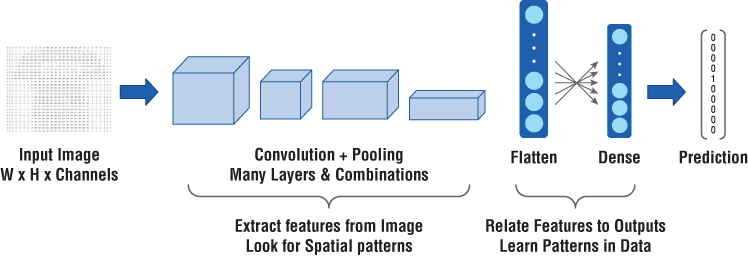
Figure 5.8: Typical CNN architecture where early layers extract spatial patterns and final dense layers learn from them
If we have a popular and proven architecture that's trained on a good diverse dataset like ImageNet, we know that this is very good at extracting features from image data—basically three‐dimensional pixel value arrays. Now if we can use this feature‐extractor and apply to our dataset, we can focus mainly on training the model to learn patterns in extracted features and relating them to desired outcomes. This greatly cuts down on our model development and training time. This is accomplished through transfer learning.
Let's dive into an example using data augmentation and transfer learning.
A Real Classification Problem: Pepsi vs. Coke
Let's take a real example to show the value of data augmentation and transfer learning during the Deep Learning model development process. Say we have a few images of the product logos of Pepsi and Coca‐Cola (Coke). We want to build a basic Deep Learning classifier that can read an image and tell us if it is a logo of Pepsi or Coke.
You see that this is a classification problem on image data. A typical first step in such a problem is to collect thousands of images of the intended classes—Coke and Pepsi logos. These should cover all the variations in size, color, shapes, viewing angle, rotation, etc. Ultimately, we should train a classifier that can take any image containing a prominent logo of Pepsi or Coke and tell us which logo it is. It is a simple binary classification problem.
As we discussed in Chapter 1, we need to always consider an analytic in the context of the system it will be used in. Here, assume that the system is a mobile app where we will use a smartphone to take a photo and somehow call our trained model to get a classification on what the image contains—Pepsi or Coke. Since it's binary classification, our output will be a single digit—0 or 1. We can say 0 will indicate Coke and 1 will indicate Pepsi. We can choose any way of naming it, as long as we use this way to feed training data to our model. So, if we choose Coke = 0 and Pepsi = 1, then all our training images for Coke should be marked 0 and Pepsi should be 1.
Now from the problem context, we can see that we may be using the cell phone at any angle to take pictures. Thus, we need to take training images from several different angles. Collecting this data seems a lot of work even for just two classes of images. This where we will use data augmentation to save time. We will take a few images—five training and five validation images for each class. Then we will use these limited datasets to convert thousands of images for training. During augmentation, we will use the contextual knowledge of the application to set parameters for how the images should be augmented.
Luckily, Keras provides some very good tools for image data augmentation. Figure 5.9 shows the folder structure we have created along with couple sample images for the logos in two classes. This is what we will feed to our Keras image augmentation methods. You see that there are two main folders, one for training and one for validation datasets. Each has folders representing the two classes we want to train for—in this case Pepsi and Coca‐Cola. Keras tools are smart enough to observe this folder structure and pick the two classes. For other problems, we can increase the number of folders inside the training and validation folders.

Figure 5.9: General folder structure for our problem of predicting two classes for images. Sample logo images from each class are shown.
I pretty much scraped these images from the web and put them in folders. They don't need to have the exact same width and height, but it's recommended that they be similar in ratio. Ultimately Keras data augmentation tools will convert these images to a standard width and height you specify. If the saved images are too different, they may look distorted.
You see that for training we just use five images of each class. We have similar images for validation also. It's highly recommended that for validation you use images that you will feed to your model in the actual application. If you are building a mobile app that will predict logos, it's better to use many mobile images from different orientations and zoom as validation images. It's usually recommended to apply data augmentation to training data and try to keep the validation data fixed. You may apply a very basic filter like scaling for this data, as we will do in the following example. I have made this small dataset with the folder structure available as a downloadable ZIP file in my S3 bucket. If you are using Google Colaboratory to run code, you can download and extract it using the commands shown in Listing 5.10.
Now we have the training and validation folders with a few images in each class. We will see how to use them in the code in Listing 5.11. We will create new images from our sample images by augmenting a few parameters and display these new augmented images on‐screen. This will give you a good idea of how this works. You can use data augmentation independently of Deep Learning to generate new images based on the existing ones.
Here are the results:
Found 10 images belonging to 2 classes. It's generating images now, as shown in Figure 5.10.

Figure 5.10: Results of data augmentation on a few logos
This is how you can generate thousands of images from a few sample images using data augmentation. You can experiment with the different generator settings to change the amount of variation that will exist in generated images. Augmentation is a very powerful feature and many other tools are available that can augment images. You can evaluate them and see what unique features they offer.
Now let's build our classification model for predicting the two logo classes. We will start with the VGG16 pretrained model like the earlier example. Now we will use transfer learning to reuse this model for our specific classification example. We will load the model in what Keras calls “headless” mode, so it will only load the feature‐extractor layers and not the fully‐connected learning layers. We will build our own fully‐connected layers to learn patterns on our data. Let's see how, in Listing 5.12.
Here are the results:
_________________________________________________________________Layer (type) Output Shape Param #=================================================================input_2 (InputLayer) (None, 150, 150, 3) 0_________________________________________________________________block1_conv1 (Conv2D) (None, 150, 150, 64) 1792_________________________________________________________________block1_conv2 (Conv2D) (None, 150, 150, 64) 36928_________________________________________________________________block1_pool (MaxPooling2D) (None, 75, 75, 64) 0_________________________________________________________________block2_conv1 (Conv2D) (None, 75, 75, 128) 73856_________________________________________________________________block2_conv2 (Conv2D) (None, 75, 75, 128) 147584_________________________________________________________________block2_pool (MaxPooling2D) (None, 37, 37, 128) 0_________________________________________________________________block3_conv1 (Conv2D) (None, 37, 37, 256) 295168_________________________________________________________________block3_conv2 (Conv2D) (None, 37, 37, 256) 590080_________________________________________________________________block3_conv3 (Conv2D) (None, 37, 37, 256) 590080_________________________________________________________________block3_pool (MaxPooling2D) (None, 18, 18, 256) 0_________________________________________________________________block4_conv1 (Conv2D) (None, 18, 18, 512) 1180160_________________________________________________________________block4_conv2 (Conv2D) (None, 18, 18, 512) 2359808_________________________________________________________________block4_conv3 (Conv2D) (None, 18, 18, 512) 2359808_________________________________________________________________block4_pool (MaxPooling2D) (None, 9, 9, 512) 0_________________________________________________________________block5_conv1 (Conv2D) (None, 9, 9, 512) 2359808_________________________________________________________________block5_conv2 (Conv2D) (None, 9, 9, 512) 2359808_________________________________________________________________block5_conv3 (Conv2D) (None, 9, 9, 512) 2359808_________________________________________________________________block5_pool (MaxPooling2D) (None, 4, 4, 512) 0_________________________________________________________________flatten_1 (Flatten) (None, 8192) 0_________________________________________________________________dense_1 (Dense) (None, 512) 4194816_________________________________________________________________dropout_1 (Dropout) (None, 512) 0_________________________________________________________________dense_2 (Dense) (None, 64) 32832_________________________________________________________________dense_3 (Dense) (None, 1) 65=================================================================Total params: 18,942,401Trainable params: 4,227,713Non‐trainable params: 14,714,688_________________________________________________________________
Notice the earlier layers in the model are the same as VGG16. We added the later layers flatten_1, dense_1, dense_2, and dense_3. Dense_3 has just one output neuron signifying our output, which can be 0 or 1 based on the image being a Coca‐Cola or Pepsi logo. Notice that we also include a dropout layer, where 50% of the neurons get dropped so that the model does not overfit on training data. This is very important since we have limited training data and are generating new images only through augmentation. Overfitting can be a problem here.
Now let's use these generators to directly feed data to the model and train it. We will also create a validation generator that will not use a whole lot of augmentation. We will only scale the image so that the pixel values are between 0 and 1 for ease of learning. See Listing 5.13.
Here are the results:
Found 10 images belonging to 2 classes. Our validation folder also has five images of each class for validation. We don't use any augmentation and just use rescaling to load these images. That's a recommended practice.
Now we will use a single line of code to apply both our training and validation generators to our model and do the training. We will use one thousand steps per epoch for training, which means we will generate one thousand images and use them for training. For validation, we will generate one hundred images. We will run the training for two epochs only. Here we go, as shown in Listing 5.14.
Here are the results:
Epoch 1/21000/1000 [==============================] ‐ 32s 32ms/step ‐ loss:0.2738 ‐ acc: 0.9490 ‐ val_loss: 0.7044 ‐ val_acc: 0.8000Epoch 2/21000/1000 [==============================] ‐ 28s 28ms/step ‐ loss:0.0156 ‐ acc: 0.9970 ‐ val_loss: 1.6118 ‐ val_acc: 0.9000
You can see that our training data accuracy is pretty high. For validation data, the accuracy keeps improving over the epoch. We can get much better accuracy by getting more data and using a good representative set for training as compared to validation.
Now let's make a couple of predictions using our trained model, as shown in Listing 5.15.
Now we have a pretty good model that can tell two logos apart. Let's look at some testing done in Figure 5.11.

Figure 5.11: Predictions for test1.jpg: Coca‐Cola and test2.jpg: Pepsi
We will save this as a model file. Keras uses the HDF5 or H5 format to store data. This is the Hierarchical Data Format (HDF), which is good at storing arrays. Some other engines may store models as JSON or YAML files. When we save models, we are saving two things—the architecture of the network and the weights associated with it. The one containing the weights is usually the bigger file. With H5 you can save both in a single file. See Listing 5.16.
Now we load this saved model into a new variable and use this to make predictions about a new image, just as we did earlier. See Listing 5.17.
There you have it. We have a model that is trained to “see” images and tell us if the image contains a logo of Coca‐Cola or of Pepsi. This can be used on new images to make predictions on what logo is present in them.
Recurrent Neural Networks
So far, we looked at image data and how to build neural networks for decoding patterns from images. Convolutional Neural Networks (CNN) is the proven architecture for extracting knowledge from image data. As we learned in Chapter 3, another common type of unstructured data is text data. Text data comes as a sequence of words and, to analyze this data, special kinds of networks are required. These are not the feed‐forward kind, where each layer is connected only to the next network layer. The new architecture we look at is called a recurrent neural network (RNN). Figure 5.12 shows this architecture.

Figure 5.12: Architecture of a Recurrent Neural Network
(Source: François Deloche – Wikipedia)
Recurrent networks don't have all forward‐feeding connections. At each layer, the output value is tapped and fed back to the next input in the sequence. Hence, the input for this network comes from the sequence and the value coming back from the previous layer. This is illustrated in Figure 5.12, by unfolding the network to show values over a sequence of time steps—Xt‐1, Xt, Xt+1. Due to this characteristic of passing part of the value from the previous item in the sequence to the next, this network can remember key values while it's learning. This is very much like how our human brain processes sequences. When we interpret sequences like text or speech, we remember previous information and use it to make sense of future values. For example, I am sure you remember items like neural networks from previous chapters and hopefully that's helping you interpret this new knowledge.
One problem with RNN is that it cannot remember values for a long time. This is where a special type of RNN, called Long Short‐Term Memory (LSTM), comes in handy. LSTM uses a gated architecture to remember key items over long sequences. We will not go into details of the gated architecture of LSTM but I do provide references at end of the book on this topic. We can use LSTM layers as a new type of layer in Keras that will work well with sequence data like text.
We talked in Chapter 3 about how text is represented. We saw that we could take a body of text like a sentence as an integer array based on the vocabulary of all words used. Then we can convert this array into dense word embeddings for each word in the sequence. We saw how these word embeddings capture the context of using these words and helps us do word math.
Now we will convert the words into embeddings and feed these as a sequence to our LSTM model to learn information. We will handle a particular case study to detect sentiments in sentences. Sentences can have a positive or negative sentiment, depending on the type and order of words used to form them.
We will first use a dataset available in Keras, called IMDB. This is a dataset of movie reviews that's been converted into integer arrays using a standard vocabulary. We will use a Keras embeddings layer to convert these integers into word embedding vectors and learn how to classify sentiments. Then we will run the same example on our own text and see if it predicts the sentiment correctly. Let's get started.
First, we load the dataset and explore it. As mentioned, the sentences come as an integer array along with a label of positive or negative for the sentiment. Let's explore the data in Listing 5.18.
Here are the results:
Loading data…Pad sequences (samples x time)x_train shape: (25000, 50)x_test shape: (25000, 50)
Now we will explore the data. We will see the integer array and use vocabulary to get the full sentences. Let's look at this in Listing 5.19.
Here are the results:
Sample of x_train array = [2071 56 26 141 6 194 7486 18 4226 22 21 134 476 26 480 5 144 30 5535 18 51 3628 224 92 25 104 4 226 65 16 38 1334 88 12 16 2835 16 4472 113 103 32 15 16 5345 19 178 32]Sample of y_train array = 1Vocabulary = {'with': 16, 'i': 10, 'as': 14, 'it': 9, 'is': 6, 'in': 8,'but': 18, 'of': 4, 'this': 11, 'a': 3, 'for': 15, 'br': 7, 'the': 1,'was': 13, 'and': 2, 'to': 5, 'film': 19, 'movie': 17, 'that': 12}-------------------------SOME SENTENCE AND SENTIMENT SAMPLES-------------------------Training Sentence = grown up are such a big profile for the whole film but these children are amazing and should be praised for what they have done don't you think the whole story was so lovely because it was true and was someone's life after all that was shared with us allSentiment = Positive-----------------------Training Sentence = taking away bodies and the gym still doesn't close for <UNK> all joking aside this is a truly bad film whose only charm is to look back on the disaster that was the 80's and have a good old laugh at how bad everything was back thenSentiment = Negative-----------------------Training Sentence = must have looked like a great idea on paper but on film it looks like no one in the film has a clue what is going on crap acting crap costumes i can't get across how <UNK> this is to watch save yourself an hour a bit of your lifeSentiment = Negative-----------------------Training Sentence = man to see a film that is true to Scotland this one is probably unique if you maybe <UNK> on it deeply enough you might even re evaluate the power of storytelling and the age old question of whether there are some truths that cannot be told but only experiencedSentiment = Positive-----------------------Training Sentence = the <UNK> and watched it burn and that felt better than anything else i've ever done it took American psycho army of darkness and kill bill just to get over that crap i hate you sandler for actually going through with this and ruining a whole day of my lifeSentiment = Negative-----------------------
Now we will build the model and do the training. Notice the use of the embedding and LSTM layers instead of the previous Conv2D and Dense layers. See Listing 5.20.
Here are the results:
Train on 25000 samples, validate on 25000 samplesEpoch 1/225000/25000 [==============================] ‐ 126s 5ms/step ‐ loss:0.4600 ‐ acc: 0.7778 ‐ val_loss: 0.3969 ‐ val_acc: 0.8197Epoch 2/225000/25000 [==============================] ‐ 125s 5ms/step ‐ loss:0.2914 ‐ acc: 0.8780 ‐ val_loss: 0.4191 ‐ val_acc: 0.811925000/25000 [==============================] ‐ 26s 1ms/stepTest score: 0.41909076169013976Test accuracy: 0.81188
We will save the model as an H5 file called imdb_nlp.h5. We will not use the saved model file right away. We will use this file in Chapter 8 (“Deploying AI Models as Microservices”). For now, we will use the trained model in memory to predict new text. We see that prediction will be a value between 0 and 1. If the value is close to 0, the sentiment is positive. Otherwise, it's negative. See Listing 5.21.
Here are the results:
SENTENCE : really bad experience. amazingly bad. :0.8450574 : SENTIMENT : NegativeSENTENCE : pretty awesome to see. very good work. :0.21833718 : SENTIMENT : Positive
There you have it. We classified images to detect logos and classified text to identify the sentiment of the sentences. There is a lot more to Deep Learning and Keras than what we covered in this chapter. We have just scraped the surface. Hopefully I have stirred your interest in this area and given you enough to start playing in this field with your own datasets. By using tools like Google Colaboratory, you can run your code on the best of hardware environments like GPU and TPU without any cost. All the best!
Summary
In this chapter, we moved from the basics into some advanced concepts in Deep Learning. We looked at concepts like data augmentation and transfer learning, which can help you work with limited data and reuse knowledge from existing proven model architectures. We also saw an example of building a model to learn about image data containing product logos and used it to make real‐world predictions.
We will now take a break from Deep Learning. The next chapter starts looking at the history of software applications and how microservices and Cloud applications are developed using containers. We will explore Kubernetes, which is fast becoming the platform of choice for managing lifecycles of containers and providing a Container‐as‐a‐Service paradigm. Modern applications—especially Cloud‐native ones—get packaged as containers and can be scheduled by Kubernetes. We will see all this magic in the next chapter.