10
Universal Intervals: Towards a Dependency‐Aware Interval Algebra
Hend Dawoodand1 and Yasser Dawood2
1Department of Mathematics, Faculty of Science, Cairo University, Giza, 12613, Egypt
2Department of Astronomy, Faculty of Science, Cairo University, Giza, 12613, Egypt
The most reliable way of carrying out a proof, obviously, is to follow pure logic, a way that, disregarding the particular characteristics of objects, depends solely on those laws upon which all knowledge rests.
–Gottlob Frege (1848–1925)
10.1 Introduction
Scientific knowledge is not perfect exactitude: it is learning with uncertainty, not eliminating it. We commit errors. But, indeed, we can grasp, measure, and correct our errors and develop ways to deal with uncertainty, which add to our knowledge and make it valuable. Knowledge, then, is not absolute certainty. Knowledge, per contra, is “the tools we develop to purposely get better and better outcomes through our learning about the world” [1]. Many approaches were developed with a view to cope with uncertainty and get reliable knowledge about the world. As examples of these approaches, we can mention probabilitization, fuzzification, and intervalization. For the great degree of reliability it provides, and because of its great importance in many practical applications, intervalization is usually a part of all other methods that deal with uncertainty (see [1] and [2]). Whenever uncertainty exists, there is always a need for interval computations and intervals arise naturally in a wide variety of disciplines that deal with uncertain data. It is a natural and elegant idea that of expressing uncertain real‐valued quantities as real closed intervals. In this very simple and old idea, the field of interval mathematics has its roots from the Greek mathematician Archimedes of Syracuse (287–212 BCE), who used guaranteed lower and upper bounds to compute his constant ![]() [3], to the American mathematician Ramon Edgar Moore (1929–2015), who was the first to define interval analysis in its modern sense and recognize its power as a viable computational tool for intervalizing uncertainty [4]. In between, historically speaking, several distinguished constructions of interval arithmetic by John Charles Burkill, Rosalind Cecily Young, Paul S. Dwyer, Teruo Sunaga, and others (see, e.g. [5–8]) have emphasized the very idea of reasoning about uncertain values through calculating with intervals. By integrating the complementary powers of rigorous mathematics and scientific computing, interval arithmetic is able to offer highly reliable accounts of uncertainty. It should therefore come as no surprise that the interval theory has been fruitfully applied in diverse areas that deal intensely with uncertain quantitative data (see, e.g. [2,9–12]).
[3], to the American mathematician Ramon Edgar Moore (1929–2015), who was the first to define interval analysis in its modern sense and recognize its power as a viable computational tool for intervalizing uncertainty [4]. In between, historically speaking, several distinguished constructions of interval arithmetic by John Charles Burkill, Rosalind Cecily Young, Paul S. Dwyer, Teruo Sunaga, and others (see, e.g. [5–8]) have emphasized the very idea of reasoning about uncertain values through calculating with intervals. By integrating the complementary powers of rigorous mathematics and scientific computing, interval arithmetic is able to offer highly reliable accounts of uncertainty. It should therefore come as no surprise that the interval theory has been fruitfully applied in diverse areas that deal intensely with uncertain quantitative data (see, e.g. [2,9–12]).
In view of this computational power against error, machine realizations of interval arithmetic are of great importance. It should therefore come as no surprise that there are many software implementations of interval arithmetic. As instances, we may mention INTLAB, Sollya, InCLosure, and others (see, e.g. [13–16]). Fortunately, computers are getting faster, and most existing parallel processors provide a tremendous computing power. Therefore, with little extra hardware, it is very possible to make interval computations as fast as floating point computations (for further reading about machine arithmetizations and hardware circuitries for interval arithmetic, see, e.g. [17–22]).
The intended status of the present work is thus to be both an in‐depth introduction and a treatise on the philosophical, mathematical, and practical aspects of interval mathematics. In the body of the work, there is room for novelties which may not be devoid of interest to researchers and specialists. The theories of classical intervals and parametric intervals are formally constructed, and their mathematical structures are uncovered. The notion of interval dependency is formalized by putting on a systematic basis its meaning and thus gaining the advantage of indicating formally the criteria by which it is to be characterized and, accordingly, deducing its fundamental properties in a merely logical manner. Moreover, with a view to treating some problems of the present interval theories, a new alternate theory of intervals, namely, the “theory of universal intervals,” is presented and proved to have a nice S‐field algebra, which extends the ordinary field of the reals.
A number of problems of interval mathematics have motivated the treatise presented in the body of this work. In the first place, in the interval literature, some important parts of interval mathematics are handled in a vaguely naïve manner without formalizing their underlying foundations. These parts are present as basic and indispensable ingredients of both fundamental research and practical applications. This work is rather different in approach and perspective. Our approach is formal, by the pursuit of formulating the mathematical concepts in a strictly accurate manner. Our perspective is to put on a systematic basis the fundamental notions of interval mathematics by taking the passage from the ambiguous and naïve treatments to the formal technicalities of mathematical logic.
In the second place, a main drawback of interval mathematics is the persisting problem known as the “interval dependency problem.” This, naturally, confronts us with the question: Formally, what is interval dependency? Is it a metaconcept or an object ingredient of interval and fuzzy computations? In other words, what is the fundamental defining properties that characterize the notion of interval dependency as a formal mathematical object? Since the early works on interval mathematics by Burkill [5] and Young [6] in the dawning of the twentieth century, this question has never been touched upon and remained a question still today unanswered. Although the notion of interval dependency is widely used in the interval and fuzzy literature, it is only illustrated by example, without explicit formalization, and no attempt has been made to put on a systematic basis its meaning, that is, to indicate formally the criteria by which it is to be characterized. Here, we attempt to answer this long‐standing question.
In the third place, the theory of parametric interval arithmetic has an underlying idea that seems elegant and simple, but it is too simple to fully account for the notion of interval dependency or to achieve a richer algebraic structure for interval arithmetic. It is therefore imperative both to supply the defect in the parametric approach and to present an alternative theory with a mathematical construction that avoids the defect.
Our approach is formal, our perspective is systematic, but our concern is practical. We describe, in detail, a number of examples that clarify the need for interval computations to cope with uncertainty in real‐world systems. The InCLosure commands1 to compute the results of the examples are described and an InCLosure input file and its corresponding output containing, respectively, the code and results of the examples are also available as a supplementary material to this chapter (see Supplementary Materials). Also, for the text to be self‐contained, and with an eye towards making the adopted formal approach clearly comprehensible, our formalized apparatus is fixed early in Section 10.3, before moving on to main business of the text. In Section 10.4, we give a systematic characterization of the classical interval theory as a many‐sorted algebra over the real field. In Section 10.5, we attempt to answer the long‐standing question concerning the defining properties that characterize the notion of interval dependency as a formal mathematical object. We present a complete systematic formalization of the notion of interval dependency, by means of the notions of Skolemization and logical quantification dependence. A novelty of this formalization is the expression of interval dependency as a logical predicate (or relation) and thus gaining the advantage of deducing its fundamental properties in a merely logical manner. This result sheds new light on many problems of interval mathematics. Moreover, a breakthrough behind our formalization of interval dependency is that it paves the way and provides the systematic apparatus for developing alternate dependency‐aware interval theories and computational methods with mathematical constructions that better account for dependencies between the quantifiable uncertainties of the real world. The objective of Section 10.7 is to introduce the theory of parametric intervals and to mathematically examine to what extent it accomplishes its objectives. Based on our formalization of the notion of interval dependency, we attempt, in Sections 10.8 and 10.9, to present an alternate theory of intervals, namely, the “theory of universal intervals,” with a mathematical construction that tries to avoid some of the defects in the current theories of interval arithmetic, to provide a richer interval algebra, and to better account for the notion of interval dependency. Finally, in Section 10.10, we discuss some further consequences and future prospects concerning the results presented in this chapter.
10.2 The Need for Interval Computations
When modeling and predicting real‐life or physical phenomena, we face the problem of uncertainty in quantifiable properties. Tackling such uncertainties introduces two different problems: getting guaranteed bounds of the exact value of a quantifiable property and computing an approximation of the value. The two problems are very different. In many practical applications, the numerical approximations provided by machine real arithmetic are not beneficial. In robotics and control applications, for example, it is important to have guaranteed inclusions of the exact values in order to guarantee stability under uncertainty [1]. The two problems are not equivalent. The implication “getting guaranteed bounds ![]() computing approximations” is true, but the converse implication is not. Interval arithmetic provides us a reliable way to get guaranteed bounds when modeling physical systems under uncertainty. An interval number (a real closed interval) is then a reliable enclosure of an uncertain real‐valued quantity, and an interval function is accordingly a reliable enclosure of an uncertain real‐valued function.
computing approximations” is true, but the converse implication is not. Interval arithmetic provides us a reliable way to get guaranteed bounds when modeling physical systems under uncertainty. An interval number (a real closed interval) is then a reliable enclosure of an uncertain real‐valued quantity, and an interval function is accordingly a reliable enclosure of an uncertain real‐valued function.
In order to further clarify the need for the guaranteed enclosures of interval arithmetic, we provide here a brief discussion of the limitations and loss of precision of machine real arithmetic. Machine real numbers have finite decimal places of precision. The finite precision provided by modern computers is enough in many real‐life applications, and there is scarcely a physical quantity which can be measured beyond the maximum representable value of this precision. So when is the finite precision not enough? The problem arises when doing arithmetic. The operation of “subtraction,” for example, results, in many situations, in an inevitable loss of precision. Consider, for instance, the expression ![]() , with
, with ![]() and
and ![]() . The exact result of
. The exact result of ![]() is 0.001, but when evaluating this expression on a machine with two significant digits, the values of
is 0.001, but when evaluating this expression on a machine with two significant digits, the values of ![]() and
and ![]() are rounded downward to have the same machine value 0.96, and the machine result of
are rounded downward to have the same machine value 0.96, and the machine result of ![]() becomes 0, which is a complete loss of precision. Instead, by enclosing the exact values of
becomes 0, which is a complete loss of precision. Instead, by enclosing the exact values of ![]() and
and ![]() in interval numbers, with outward rounding, a guaranteed enclosure of the exact result of
in interval numbers, with outward rounding, a guaranteed enclosure of the exact result of ![]() can be obtained easily by computing with machine interval numbers [18].
can be obtained easily by computing with machine interval numbers [18].
This problem of machine subtraction has dangerous consequences in numerical computations. To illustrate, consider the problem of calculating the derivative of a real‐valued function ![]() at a given point. The method of finite differences is a numerical method which can be performed by a computer to approximate the derivative. For a differentiable function
at a given point. The method of finite differences is a numerical method which can be performed by a computer to approximate the derivative. For a differentiable function ![]() , the first derivative
, the first derivative ![]() can be approximated by
can be approximated by
for a small nonzero value of ![]() . As
. As ![]() approaches zero, the derivative is better approximated. But, as
approaches zero, the derivative is better approximated. But, as ![]() gets smaller, the rounding error increases because of the finite precision of machine real arithmetic, and we accordingly get the problematic situation of
gets smaller, the rounding error increases because of the finite precision of machine real arithmetic, and we accordingly get the problematic situation of ![]() . That is, for small enough values of
. That is, for small enough values of ![]() , the derivative will be always computed as zero, regardless of the rule of the function
, the derivative will be always computed as zero, regardless of the rule of the function ![]() . Using interval enclosures of the function
. Using interval enclosures of the function ![]() instead, we can find a way out of this problem, by virtue the infinite precision of machine interval arithmetic. For further details on interval enclosures of derivatives, see, e.g. [1] and [18].
instead, we can find a way out of this problem, by virtue the infinite precision of machine interval arithmetic. For further details on interval enclosures of derivatives, see, e.g. [1] and [18].
Another problem of finite precision arises when truncating an infinite operation by a computable finite operation. For example, the exponential function ![]() may be written as a Taylor series
may be written as a Taylor series

In order to compute this infinite series on a machine, we have to truncate it to the partial sum

for some finite ![]() , and the truncation error then is
, and the truncation error then is ![]() . Using interval bounds for this error term, machine interval arithmetic can provide a guaranteed enclosure of the exact value of the exponential function
. Using interval bounds for this error term, machine interval arithmetic can provide a guaranteed enclosure of the exact value of the exponential function ![]() .
.
The preceding examples shed light on the fact that taking the passage from real arithmetic to interval arithmetic opens the way to the rich technicalities and the infinite precision of interval computations.
10.3 On Some Algebraic and Logical Fundamentals
In order to be able to give a complete systematic formalization of the notion of interval dependency and related notions, we do need readily available a formal apparatus. So, by the pursuit of a strictly accurate formulation of the mathematical concepts, some particular formal approach will be adopted to generate all the results of this work from clear and distinct elementary ideas. Therefore, before moving on to the main business of this chapter, we begin in this section by specifying some notational conventions and formalizing some purely logical and algebraic ingredients we shall need throughout this text (for further details about the notions prescribed here, the reader may consult, e.g. [1823–28]).
Most of our notions are characterized in terms of ordinals and ordinal tuples. So, we first define what an ordinal is. An ordinal is the well‐ordered set of all ordinals preceding it. That is, for each ordinal ![]() , there exists an ordinal
, there exists an ordinal ![]() called the successor of
called the successor of ![]() such that
such that
In other words, we have ![]() . Accordingly, the first infinite (transfinite) ordinal is the set
. Accordingly, the first infinite (transfinite) ordinal is the set ![]() . All ordinals preceding
. All ordinals preceding ![]() (all elements of
(all elements of ![]() ) are finite ordinals. The idea of transfinite counting (counting beyond the finite) is due to Cantor (see [29]).
) are finite ordinals. The idea of transfinite counting (counting beyond the finite) is due to Cantor (see [29]).
With the aid of ordinals, the notions of countably finite, countably infinite, and uncountably infinite sets can be characterized as follows. A set ![]() is countably finite if there is a bijective mapping from
is countably finite if there is a bijective mapping from ![]() onto some finite ordinal
onto some finite ordinal ![]() . A set
. A set ![]() is countably infinite (or denumerable) if there is a bijective mapping from
is countably infinite (or denumerable) if there is a bijective mapping from ![]() onto the infinite ordinal
onto the infinite ordinal ![]() . For example, the set
. For example, the set ![]() is countably finite because it can be bijectively mapped onto the finite ordinal
is countably finite because it can be bijectively mapped onto the finite ordinal ![]() , while the set
, while the set ![]() is denumerable because it can be bijectively mapped onto the infinite ordinal
is denumerable because it can be bijectively mapped onto the infinite ordinal ![]() . An uncountably infinite set is an infinite set which is not countably infinite. For example, the set
. An uncountably infinite set is an infinite set which is not countably infinite. For example, the set ![]() of real numbers is uncountably infinite.
of real numbers is uncountably infinite.
The notion of an ![]() ‐tuple is characterized in the following definition.
‐tuple is characterized in the following definition.
If ![]() , then, for any set
, then, for any set ![]() , there is exactly one mapping (the empty mapping)
, there is exactly one mapping (the empty mapping) ![]() from
from ![]() into
into ![]() .
.
An important definition we shall need is that of the Cartesian power of a set.
In accordance with the preceding definitions, a set‐theoretical relation is a particular type of set. Let ![]() be the binary Cartesian power of a set
be the binary Cartesian power of a set ![]() . A binary relation on
. A binary relation on ![]() is a subset of
is a subset of ![]() . That is, a set
. That is, a set ![]() is a binary relation on a set
is a binary relation on a set ![]() iff
iff ![]() .
.
We will continue to follow the formal tradition of Suppes [31] and Tarski [32] in defining, within a set‐theoretical framework, the notion of a finitary relation and some related concepts. Let ![]() be the
be the ![]() ‐th Cartesian power of a set
‐th Cartesian power of a set ![]() . A set
. A set ![]() is an
is an ![]() ‐ary relation on
‐ary relation on ![]() iff
iff ![]() is a binary relation from
is a binary relation from ![]() to
to ![]() . That is, for
. That is, for ![]() and
and ![]() , an
, an ![]() ‐ary relation
‐ary relation ![]() is defined to be
is defined to be ![]() . In this sense, an
. In this sense, an ![]() ‐ary relation is a binary relation (or simply a relation); then its domain, range, field, and converse are defined to be, respectively
‐ary relation is a binary relation (or simply a relation); then its domain, range, field, and converse are defined to be, respectively ![]() ,
, ![]() ,
, ![]() , and
, and ![]() . It is thus obvious that
. It is thus obvious that ![]() and
and ![]() .
.
Two important notions, for the purpose at hand, are the image and preimage of a set, with respect to an ![]() ‐ary relation. These are defined as follows [9] and [27].
‐ary relation. These are defined as follows [9] and [27].
In accordance with this definition and the fact that ![]() , we obviously have
, we obviously have ![]() .
.
Within this set‐theoretical framework, a completely general definition of the notion of an n‐ary function can be formulated. A set ![]() is an
is an ![]() ‐ary function on a set
‐ary function on a set ![]() iff
iff ![]() is an
is an ![]() ‐ary relation on
‐ary relation on ![]() , and
, and ![]() . Thus, an
. Thus, an ![]() ‐ary function is a many‐one
‐ary function is a many‐one ![]() ‐ary relation; that is, a relation, with respect to which, any element in its domain is related exactly to one element in its range. Getting down from relations to the particular case of functions, we have at hand the standard notation:
‐ary relation; that is, a relation, with respect to which, any element in its domain is related exactly to one element in its range. Getting down from relations to the particular case of functions, we have at hand the standard notation: ![]() in place of
in place of ![]() . From the fact that an
. From the fact that an ![]() ‐ary function is a special kind of relation, then all the preceding definitions and results, concerning the domain, range, field, and converse of a relation, apply to functions as well.
‐ary function is a special kind of relation, then all the preceding definitions and results, concerning the domain, range, field, and converse of a relation, apply to functions as well.
With some criteria satisfied, a function is called invertible. A function ![]() has an inverse, denoted
has an inverse, denoted ![]() , iff its converse relation
, iff its converse relation ![]() is a function, in which case
is a function, in which case ![]() . In other words,
. In other words, ![]() is invertible if, and only if, it is an injection from its domain to its range, and obviously, the inverse
is invertible if, and only if, it is an injection from its domain to its range, and obviously, the inverse ![]() is unique, from the fact that the converse relation is always definable and unique.
is unique, from the fact that the converse relation is always definable and unique.
By means of the above concepts, we next define the notions of partial and total operations.
A binary operation is an ![]() ‐ary operation for
‐ary operation for ![]() . Addition and multiplication on the set
. Addition and multiplication on the set ![]() of real numbers are best‐known examples of binary total operations, while division is a partial operation in
of real numbers are best‐known examples of binary total operations, while division is a partial operation in ![]() .
.
A formalized theory is characterized by two things, an object language in which the theory is formalized (the symbolism of the theory) and a set of axioms. The following metalinguistic definition characterizes the notion of a formalized theory.
A model (or an interpretation) of a theory ![]() is some particular (algebraic or relational) structure that satisfies every formula of
is some particular (algebraic or relational) structure that satisfies every formula of ![]() . The notion of a structure of a formalized language
. The notion of a structure of a formalized language ![]() (or an
(or an ![]() ‐structure) is characterized in the following definition (see [18] and [27]).
‐structure) is characterized in the following definition (see [18] and [27]).
An ![]() ‐structure with an empty individual universe is called an empty
‐structure with an empty individual universe is called an empty ![]() ‐structure.3 By a many‐sorted
‐structure.3 By a many‐sorted ![]() ‐structure, we understand an
‐structure, we understand an ![]() ‐structure with more than one universe set. By a relational
‐structure with more than one universe set. By a relational ![]() ‐structure, we understand an
‐structure, we understand an ![]() ‐structure with a nonempty set of relations and an empty set of functions. By an algebraic
‐structure with a nonempty set of relations and an empty set of functions. By an algebraic ![]() ‐structure (or an
‐structure (or an ![]() ‐algebra), we understand an
‐algebra), we understand an ![]() ‐structure with a nonempty set of functions. An
‐structure with a nonempty set of functions. An ![]() ‐algebra endowed with a compatible ordering relation
‐algebra endowed with a compatible ordering relation ![]() is called an
is called an ![]() ‐ordered
‐ordered ![]() ‐algebra.
‐algebra.
The following definition and its consequence are indispensable.
Let the mapping ![]() be an isomorphism. For each
be an isomorphism. For each ![]() , the image
, the image ![]() is called the isomorphic copy of
is called the isomorphic copy of ![]() (under the isomorphism
(under the isomorphism ![]() ).
).
That is, isomorphism is a relation between models (interpretations) of a formalized theory. To say that two models of a theory are isomorphic is to say that they have the same structural form. In this sense, the isomorphism relation is called “structural identity” by some logicians (see, e.g. [36]).
The notion of inverse elements is precisely formulated in the following definition.
We conclude this section by characterizing some algebraic structures that will be deployed as intended interpretations of the theories considered in this text.
Criteria (i) and (ii) in the preceding definition are called, respectively, left and right subdistributivity (or S‐distributivity).
Noteworthy, the notion of S‐semiring is a generalization of the notion of a near‐semiring; a near‐semiring is a ringoid that satisfies the criteria of a semiring except that it is either left or right distributive (for detailed discussions of near‐semirings and related concepts, the interested reader may consult, e.g. [37–39]).
Finally, let us close this section by making two further definitions we shall need.
10.4 Classical Intervals and the Dependency Problem
With the formalized apparatus of Section 10.3 at our disposal, the main business of this section is to give a systematic characterization of the theory ![]() of real interval arithmetic. Our adopted strategy to obtain a concrete system of classical interval numbers is to start with the field of real numbers and to “intervalize” it, by defining new interval relations and operations. In other words, the theory
of real interval arithmetic. Our adopted strategy to obtain a concrete system of classical interval numbers is to start with the field of real numbers and to “intervalize” it, by defining new interval relations and operations. In other words, the theory ![]() of real intervals will be constructed as a definitional extension of the theory of real numbers.
of real intervals will be constructed as a definitional extension of the theory of real numbers.
There are many theories of interval arithmetic (see, e.g. [17,20,40–45]). We are here interested in characterizing classical interval arithmetic as introduced in, e.g. [1,4,12,18,46], and [27]. Hereafter and throughout this work, the machinery used, and assumed priori, is the standard (classical) predicate calculus and axiomatic set theory. Moreover, in all the proofs, elementary facts about operations and relations on the real numbers are usually used without explicit reference.
A theory ![]() of a real interval algebra (a classical interval algebra or an interval algebra over the real field) is characterized in the following definition (see [1] and [27]).
of a real interval algebra (a classical interval algebra or an interval algebra over the real field) is characterized in the following definition (see [1] and [27]).
The sentence (I1) of Definition 10.15 characterizes what an interval number (or a closed ![]() ‐interval) is. The sentences (I2) and (I3) prescribe, respectively, the binary and unary operations for
‐interval) is. The sentences (I2) and (I3) prescribe, respectively, the binary and unary operations for ![]() ‐intervals. Hereafter, the uppercase Roman letters
‐intervals. Hereafter, the uppercase Roman letters ![]() ,
, ![]() , and
, and ![]() (with or without subscripts), or equivalently
(with or without subscripts), or equivalently ![]() ,
, ![]() , and
, and ![]() , shall be employed as variable symbols to denote real interval numbers. A point (singleton) interval number
, shall be employed as variable symbols to denote real interval numbers. A point (singleton) interval number ![]() shall be denoted by
shall be denoted by ![]() . The letters
. The letters ![]() ,
, ![]() , and
, and ![]() , or equivalently
, or equivalently ![]() ,
, ![]() , and
, and ![]() , shall be used to denote constants of
, shall be used to denote constants of ![]() . Also, we shall single out the symbols
. Also, we shall single out the symbols ![]() and
and ![]() to denote, respectively, the singleton
to denote, respectively, the singleton ![]() ‐intervals
‐intervals ![]() and
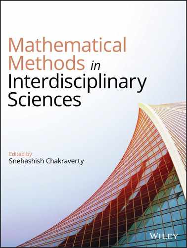
and ![]() . For the purpose at hand, it is convenient to define two proper subsets of
. For the purpose at hand, it is convenient to define two proper subsets of ![]() : the sets of symmetric interval numbers and point interval numbers. Respectively, these are defined and denoted by
: the sets of symmetric interval numbers and point interval numbers. Respectively, these are defined and denoted by
From the fact that real intervals are totally ![]() ‐ordered subsets of
‐ordered subsets of ![]() , equality of
, equality of ![]() ‐intervals follows immediately from the axiom of extensionality4 of set theory. That is,
‐intervals follows immediately from the axiom of extensionality4 of set theory. That is,
Since ![]() ‐intervals are ordered sets of real numbers, it follows that the next theorem is derivable from Definition 10.15 (see [1] and [47]).
‐intervals are ordered sets of real numbers, it follows that the next theorem is derivable from Definition 10.15 (see [1] and [47]).
Wherever there is no confusion, we shall drop the subscripts ![]() and
and ![]() . By Definition 10.4, it is obvious that all the interval operations, except interval reciprocal, are total operations. The additional operations of interval subtraction and division can be defined, respectively, as
. By Definition 10.4, it is obvious that all the interval operations, except interval reciprocal, are total operations. The additional operations of interval subtraction and division can be defined, respectively, as ![]() and
and ![]() .
.
Classical interval arithmetic has a number of peculiar algebraic properties: The point intervals ![]() and
and ![]() are identity elements for addition and multiplication, respectively; interval addition and multiplication are both commutative and associative; interval addition is cancellative; interval multiplication is cancellative only for zeroless intervals; an interval number is invertible for addition (respectively, multiplication) if and only if it is a point interval (respectively, a nonzero point interval); and interval multiplication left and right subdistributes over interval addition (see Definition 10.10). Accordingly, by Definitions 10.12 and 10.14, we have the following theorem and its corollary (see [1] and [18]).
are identity elements for addition and multiplication, respectively; interval addition and multiplication are both commutative and associative; interval addition is cancellative; interval multiplication is cancellative only for zeroless intervals; an interval number is invertible for addition (respectively, multiplication) if and only if it is a point interval (respectively, a nonzero point interval); and interval multiplication left and right subdistributes over interval addition (see Definition 10.10). Accordingly, by Definitions 10.12 and 10.14, we have the following theorem and its corollary (see [1] and [18]).
Throughout this text, we shall employ the following theorem and its corollary (see [1] and [9]).
In consequence of this theorem, from the fact that ![]() , we have the following important special case.
, we have the following important special case.
If we endow the classical interval algebra ![]() with the compatible partial ordering
with the compatible partial ordering ![]() , then we have a partially ordered commutative S‐semiring. In addition to ordering intervals by the set inclusion relation
, then we have a partially ordered commutative S‐semiring. In addition to ordering intervals by the set inclusion relation ![]() , there are many orders presented in the interval literature. Among these is Moore's partial ordering, which is defined by
, there are many orders presented in the interval literature. Among these is Moore's partial ordering, which is defined by ![]() . In contrast to the case for
. In contrast to the case for ![]() , Moore's partial ordering
, Moore's partial ordering ![]() is not compatible with the algebraic operations on
is not compatible with the algebraic operations on ![]() (see [1] and [27]).
(see [1] and [27]).
We conclude the present section with a peculiarity of interval arithmetic that seems quite strange at first. Note that the set‐theoretic characterization of the interval operations (Definition 10.15) implies that interval arithmetic considers all instances of variables as independent. Accordingly, for two interval variables ![]() and
and ![]() assigned the same interval constant
assigned the same interval constant ![]() , both the interval operations
, both the interval operations ![]() and
and ![]() are equal and they are the same as the image of the multivariate real function
are equal and they are the same as the image of the multivariate real function ![]() , with
, with ![]() and
and ![]() . In fact, this is one of the strengths of interval mathematics: because images of real functions are inclusion monotonic (see, e.g. [9,27], and [48]), it follows that the image of the function
. In fact, this is one of the strengths of interval mathematics: because images of real functions are inclusion monotonic (see, e.g. [9,27], and [48]), it follows that the image of the function ![]() is an enclosure of the image of a unary real function
is an enclosure of the image of a unary real function ![]() , with
, with ![]() , and therefore
, and therefore ![]() is a guaranteed enclosure of the image of
is a guaranteed enclosure of the image of ![]() . However, in many situations, this enclosure might be too wide to be useful. This phenomenon is known as the interval dependency problem. The notion of interval dependency and the problems thereof will be logically characterized in the next section.
. However, in many situations, this enclosure might be too wide to be useful. This phenomenon is known as the interval dependency problem. The notion of interval dependency and the problems thereof will be logically characterized in the next section.
10.5 Interval Dependency: A Logical Treatment
The notion of dependency comes from the notion of a function. There is scarcely a mathematical theory which does not involve the notion of a function. In ancient mathematics, the idea of functional dependence was not expressed explicitly and was not an independent object of research, although a wide range of specific functional relations were known and studied systematically. The concept of a function appears in a rudimentary form in the works of scholars in the Middle Ages, but only in the work of mathematicians in the seventeenth century, and primarily in those of Pierre de Fermat, Rene Descartes, Isaac Newton, and Gottfried Leibniz, did it begin to take shape as an independent concept. Later, in the eighteenth century, Euler had a more general approach to the concept of a function as “dependence of one variable quantity on another” [49]. By the year 1834, Lobachevskii was writing: “The general concept of a function requires that a function of ![]() is a number which is given for each
is a number which is given for each ![]() and gradually changes with
and gradually changes with ![]() . The value of a function can be given either by an analytic expression or by a condition which gives a means of testing all numbers and choosing one of them; or finally a dependence can exist and remain unknown” [50].
. The value of a function can be given either by an analytic expression or by a condition which gives a means of testing all numbers and choosing one of them; or finally a dependence can exist and remain unknown” [50].
In the theory of real closed intervals, the notion of interval dependency naturally comes from the idea of functional dependence of real variables. Despite the fact that dependency is an essential and useful notion of real variables, interval dependency is the main unsolved problem of the classical theory of interval arithmetic and its modern generalizations (see [1] and [27]). This, naturally, confronts us with the question: Formally, what is interval dependency? Is it a metaconcept or an object ingredient of interval and fuzzy computations? In other words, what are the fundamental defining properties that characterize the notion of interval dependency as a formal mathematical object? Since the early works on interval mathematics by Burkill [5] and Young [6] in the dawning of the twentieth century, this question has never been touched upon and remained a question still today unanswered. Although the notion of interval dependency is widely used in the interval and fuzzy literature, it is only illustrated by example, without explicit formalization, and no attempt has been made to put on a systematic basis its meaning, that is, to formally indicate the criteria by which it is to be characterized. Here, we attempt to answer this long‐standing question. This section, therefore, is devoted to presenting a complete systematic formalization of the notion of interval dependency by means of the notions of Skolemization and logical quantification dependence. A novelty of this formalization is the expression of interval dependency as a logical predicate (or relation) and thus gaining the advantage of deducing its fundamental properties in a merely logical manner. This result sheds new light on many problems of interval mathematics. Moreover, a breakthrough behind our formalization of interval dependency is that it paves the way and provides the systematic apparatus for developing alternate dependency‐aware interval theories and computational methods with mathematical constructions that better account for dependencies between quantifiable uncertainties of the real world.
So, in Section 10.5.1, we delve deep into some semantical and syntactical fundamentals concerning the logical formulation of the notion of functional dependence and some related notions. In Section 10.5.2, we put on a systematic basis the notion of interval dependency. This systematic basis shall play an essential role in our discussion of the interval theory, in the present section and later on.5 Based on the logical machinery presented here, we attempt, in Sections 10.8 and 10.9, to present an alternate theory of intervals, namely, the “theory of universal intervals,” with a mathematical construction that tries to avoid some of the defects in the current theories of interval arithmetic and to better account for the notion of interval dependency.
10.5.1 Quantification Dependence and Skolemization
In order to be able to formalize the notion of interval dependency, we delve deep, in this section, into some semantical and syntactical fundamentals concerning the logical formulation of the notion of functional dependence and some related notions.
When scientists observe the world to formulate the defining properties of some physical phenomenon, these defining properties figure as attributes (variables) depending on some other attributes. Translating this dependence into a formal mathematical language gives rise to the notion of functional dependence: “a variable ![]() is absolutely determined by some given variables
is absolutely determined by some given variables ![]() ,” or “a variable
,” or “a variable ![]() is a function of some given variables
is a function of some given variables ![]() ,” symbolically
,” symbolically ![]() . In some cases, such a translation can deterministically result in a certain rule for the function
. In some cases, such a translation can deterministically result in a certain rule for the function ![]() , for instance,
, for instance, ![]() . In other cases, we have an approximate rule for
. In other cases, we have an approximate rule for ![]() , or we know that a dependence exist, but the rule cannot be determined, in which case, we write the general usual notation
, or we know that a dependence exist, but the rule cannot be determined, in which case, we write the general usual notation ![]() , without specifying explicitly a rule for the function
, without specifying explicitly a rule for the function ![]() . Therefore, in mathematics, a dependence is formally a function (for further exhaustive details about the notion of dependence, from the logical and epistemological viewpoints, see, e.g. [24,51–53], and [27]).
. Therefore, in mathematics, a dependence is formally a function (for further exhaustive details about the notion of dependence, from the logical and epistemological viewpoints, see, e.g. [24,51–53], and [27]).
As is well known, the most elementary part of all mathematical sciences is formal logic. Therefore, getting down to the most elementary fundamentals, it can be clarified that in all mathematical theories, any type of dependence can be reduced to the following simple logical definition (see, e.g. [9] and [27]).
That is, the order of quantifiers in a quantification matrix determines the mutual dependence between the variables in a sentence.
Let us illustrate this by the following two examples.
By means of a Skolem equivalent form or a Skolemization,8 a quantification dependence is translated into a functional dependence. The notion of a Skolem equivalent form is characterized in the following definition (see, e.g. [27,55], and [53]).
It comes therefore as no surprise that in all mathematics, any instance of a dependence is, in fact, a functional dependence.
In order to clarify the matters, let us consider the following example.
10.5.2 A Formalization of the Notion of Interval Dependency
With the logical and set‐theoretical fundamentals of Sections 10.3 and 10.5.1 at our disposal, this section is devoted to presenting a formalized treatment of the notion of interval dependency, that is, putting on a systematic basis its meaning and thus gaining the advantage of indicating formally the criteria by which it is to be characterized and, accordingly, deducing its fundamental properties in a merely logical manner.
Before we proceed, it is convenient here to introduce some notational conventions. By a finitary real‐valued function in real arguments (in short, a real function or ![]() ‐function), we understand a function
‐function), we understand a function ![]() , and by an interval function (or
, and by an interval function (or ![]() ‐function), we understand a function
‐function), we understand a function ![]() . The
. The ![]() ‐subscripted letters
‐subscripted letters ![]() shall be employed to denote real‐valued functions, while the
shall be employed to denote real‐valued functions, while the ![]() ‐subscripted letters
‐subscripted letters ![]() shall be employed to denote interval‐valued functions. If the type of function is clear from its arguments, and if confusion is not likely to ensue, we shall usually drop the subscripts “
shall be employed to denote interval‐valued functions. If the type of function is clear from its arguments, and if confusion is not likely to ensue, we shall usually drop the subscripts “![]() ” and “
” and “![]() .” Thus, we may, for instance, write
.” Thus, we may, for instance, write ![]() and
and ![]() for, respectively, a real‐valued function and an interval‐valued function, both of which are defined by the same rule.
for, respectively, a real‐valued function and an interval‐valued function, both of which are defined by the same rule.
An important notion we shall need is that of the image set of real closed intervals, under an ![]() ‐ary real‐valued function. This notion is a special case of that of the corresponding
‐ary real‐valued function. This notion is a special case of that of the corresponding ![]() ‐ary relation on
‐ary relation on ![]() . More precisely, we have the following definition.
. More precisely, we have the following definition.
The fact formulated in the following theorem is well‐known (see, e.g. [9] and [27]).
An immediate consequence of Definition 10.18 and Theorem 10.5 is the following important property [27].
A cornerstone result from the above theorem, that should be stressed at once, is that the best way to evaluate the accurate image of a continuous real‐valued function is to apply minimization and maximization directly to determine the exact lower and upper endpoints of the image. For rational10 real‐valued functions, this optimization problem is, in general, computationally solvable, by applying Tarski's algorithm, which is also known as Tarski's real quantifier elimination (see, e.g. [56] and [57]). For algebraic11 real‐valued functions, the problem is computable, by applying the cylindrical algebraic decomposition algorithm (CAD algorithm, or Collins' algorithm),12 which is a more effective version of Tarski's algorithm (see, e.g. [59] and [60]).
Before turning to the notion of interval dependency, we first prove the following indispensable result.
From the fact that existential quantification over a nonempty set ![]() defines a set
defines a set ![]() such that
such that ![]() , the previous theorem entails, as a special case, the following important result of real analysis.
, the previous theorem entails, as a special case, the following important result of real analysis.
The following example makes the statement of Theorem 10.7 clear.
Next, we define the notion of an exact (or generalized) interval operation.
We then have the following obvious result for the classical interval operations.
With the help of the preceding notions and the deductions from them, we are now ready to pass to our formal characterization of the notion of interval dependency.
From now on, and throughout the text, the following notational convention shall be adopted. We write ![]() (with the subscript
(with the subscript ![]() ) to mean that
) to mean that ![]() is dependent on
is dependent on ![]() by some given dependency function
by some given dependency function ![]() , and we write
, and we write ![]() to mean that
to mean that ![]() and
and ![]() are mutually independent. In general, the notation
are mutually independent. In general, the notation ![]() shall be employed to mean “all
shall be employed to mean “all ![]()
![]() are pairwise mutually independent.” Hereafter, for simplicity of the language, we shall always make use of the following abbreviation.
are pairwise mutually independent.” Hereafter, for simplicity of the language, we shall always make use of the following abbreviation.
So, to say that an interval variable ![]() is dependent on an interval variable
is dependent on an interval variable ![]() , we must be given some real‐valued function
, we must be given some real‐valued function ![]() such that
such that ![]() is the image of
is the image of ![]() under
under ![]() . This characterization of interval dependency is completely compatible with the concept of functional dependence of real variables: for two real variables
. This characterization of interval dependency is completely compatible with the concept of functional dependence of real variables: for two real variables ![]() and
and ![]() , the variable
, the variable ![]() is functionally dependent on
is functionally dependent on ![]() if there is some given function
if there is some given function ![]() such that
such that ![]() , and to keep the dependency information, between
, and to keep the dependency information, between ![]() and
and ![]() , in an algebraic expression
, in an algebraic expression ![]() , it suffices to write
, it suffices to write ![]() . If
. If ![]() and
and ![]() are mutually dependent by an idempotence
are mutually dependent by an idempotence ![]() and
and ![]() , then, to keep the dependency information, it suffices to write either
, then, to keep the dependency information, it suffices to write either ![]() or
or ![]() . In case there is neither such a given function
. In case there is neither such a given function ![]() nor such a given function
nor such a given function ![]() , then it is obvious that the real variables
, then it is obvious that the real variables ![]() and
and ![]() are not functionally dependent. Definition 10.20 extends this concept to the set of real closed intervals.
are not functionally dependent. Definition 10.20 extends this concept to the set of real closed intervals.
The preceding definition, along with two deductions that we shall presently make (Theorem 10.9 and Corollary 10.4), touches the notion of interval dependency in a way which copes with all possible cases. This shall be shown, in detail, in Sections 10.7 and 10.8. For now, to illustrate, let us give the following example.
This example shows that if two interval variables ![]() and
and ![]() both are assigned the same individual constant (both have the same value), it does not necessarily follow that
both are assigned the same individual constant (both have the same value), it does not necessarily follow that ![]() and
and ![]() are identical, unless they are dependent by the identity Function.13 This shall be made precise in Definition 10.27.
are identical, unless they are dependent by the identity Function.13 This shall be made precise in Definition 10.27.
As a consequence of our characterization of interval dependency, we have the next immediate theorem that establishes that the interval dependency relation is a quasi‐ordering relation.
In accordance with this theorem and Definition 10.19, we also have the following corollary.
The interval dependency problem can now be formulated in the following theorem.
Obviously, the result ![]() , obtained using classical interval arithmetic, has an overestimation of
, obtained using classical interval arithmetic, has an overestimation of
where ![]() is the width of the interval. This overestimated result is due to the fact that the classical interval theory assumes independence of all interval variables, even when dependencies exist.
is the width of the interval. This overestimated result is due to the fact that the classical interval theory assumes independence of all interval variables, even when dependencies exist.
A numerical example is shown below.
The problem of computing the image ![]() , using interval arithmetic, is the main problem of interval computations. This problem is, in general,
, using interval arithmetic, is the main problem of interval computations. This problem is, in general, ![]() ‐hard14 (see, e.g. [62,63], and [48]). That is, for the classical interval theory, there is no efficient algorithm to make the identity
‐hard14 (see, e.g. [62,63], and [48]). That is, for the classical interval theory, there is no efficient algorithm to make the identity
always hold unless ![]() , which is widely believed to be false. However, a considerable scientific effort is put into finding a way out from the interval dependency problem. There are many special methods and algorithms, based on the classical interval theory, that successfully compute useful narrow bounds to the desirable accurate image. In the succeeding section, we shall discuss briefly how to compute useful guaranteed enclosures under interval dependency.
, which is widely believed to be false. However, a considerable scientific effort is put into finding a way out from the interval dependency problem. There are many special methods and algorithms, based on the classical interval theory, that successfully compute useful narrow bounds to the desirable accurate image. In the succeeding section, we shall discuss briefly how to compute useful guaranteed enclosures under interval dependency.
Beyond the techniques based on the classical interval theory, various proposals for possible alternate theories of interval arithmetic were introduced to reduce the dependency effect or to enrich the algebraic structure of interval numbers. Among these alternate theories of intervals, we can mention as examples: Hansen's generalized intervals, Kulisch's complete intervals, directed intervals, modal intervals, parametric intervals, and others (see, e.g. [20,40–43], and [9]). In Section 10.7, we will in‐depth investigate the theory of parametric intervals, and in Section 10.8, we will present a new alternate theory, namely, the “theory of universal intervals.”
10.6 Interval Enclosures Under Functional Dependence
In this section, we give a bit of perspective on how to compute useful interval enclosures under functional dependence. The numerical examples of this section are computed using version 2.0 of InCLosure. The InCLosure commands to compute the results of the examples are described and an InCLosure input file and its corresponding output containing, respectively, the code and results of the examples are also available as a supplementary material to this text (see Supplementary Materials).
As mentioned in the preceding section, there are many ways out of the dependency problem to get narrower enclosures. With a knowledge of regions of monotonicity, most elementary interval functions can be defined to be the exact images of the corresponding real functions. As instances, for an interval number ![]() and a non‐negative integer
and a non‐negative integer ![]() , we can define
, we can define

where ![]() is the absolute value of the interval number
is the absolute value of the interval number ![]() .
.
Applying the naive (pure) interval operations on these exact evaluations, we can get better (narrower) enclosures of the images of the algebraic combinations of the corresponding real functions. Moreover, many techniques are used to improve the results obtained from the naive method by reducing the width of the resulting interval. Among these techniques are centered forms, generalized centered forms, circular complex centered forms, Hansen's method, remainder forms, the subdivision method, and many others (see, e.g. [1,20,48,64–66], and [67]). For instance, we can get arbitrarily narrower enclosures of images of real functions using the subdivision method, which is due to Moore (see, e.g. [64] and [65]). This method can be described as follows. Let ![]() be an interval number and let
be an interval number and let ![]() be the width of
be the width of ![]() . First, we subdivide the interval
. First, we subdivide the interval ![]() into
into ![]() subintervals
subintervals ![]() such that
such that
where ![]() . Hence,
. Hence, ![]() . Then, we evaluate the interval‐valued function
. Then, we evaluate the interval‐valued function ![]() for each subinterval
for each subinterval ![]() ,
, ![]() . Accordingly, we have [1]
. Accordingly, we have [1]
That is, the subdivision method produces better enclosures than the naive method. Moreover, the larger the number of subintervals ![]() , the narrower the enclosure of the image
, the narrower the enclosure of the image ![]() . Next, we shall describe how to make use of the interval capability of InCLosure to get arbitrarily better enclosures of the images of real functions.
. Next, we shall describe how to make use of the interval capability of InCLosure to get arbitrarily better enclosures of the images of real functions.
Table 10.1 InCLosure result for different numbers of subdivisions.
| Number of subintervals | InCLosure result |
| 1 (no subdivision) | |
| 10 | |
| 50 | |
| 100 | |
| 500 | |
| 1000 |
The exact image of the corresponding real function ![]() on
on ![]() is
is ![]() . All the results of Table 10.1 are guaranteed enclosures of the exact image, and Example 10.7 clearly shows that classical interval arithmetic with the arbitrarily narrower interval results of InCLosure thus markedly surpasses the ordinary numerical methods.
. All the results of Table 10.1 are guaranteed enclosures of the exact image, and Example 10.7 clearly shows that classical interval arithmetic with the arbitrarily narrower interval results of InCLosure thus markedly surpasses the ordinary numerical methods.
10.7 Parametric Intervals: How Far They Can Go
An important and promising theory of interval arithmetic is the theory of parametric intervals. Although it is scarcely mentioned in the interval literature, if at all, parametric interval arithmetic has widespread applications in many scientific fields such as artificial intelligence, fuzzy systems, and granular computing, which require more accuracy and compatibility with the semantic of real arithmetic and fuzzy set theory (see, e.g. [56,68], and [69]).
The term “parametric interval arithmetic” is reasonably recent, but the idea perhaps has an earlier root in Cleary's “logical arithmetic” which is a logical technique, for real arithmetic in Prolog, that uses constraints over real intervals (see [70] and [71]). Over the past few decades, parametric interval arithmetic has been invented and “reinvented” several times, under different names: “logical intervals,” “constrained intervals,” “instantiation intervals,” “RDM intervals,” and “Overestimation‐free intervals” (see, e.g. [9,17,43,70,72,73], and [74]). The theory of parametric intervals is presented in the literature as an approach to solving the long‐standing dependency problem in the classical interval theory, along with the emphasis that parametric interval arithmetic, unlike Moore's classical interval arithmetic, has additive and multiplicative inverse elements and satisfies the distributive law.
Our main purpose in this section is to introduce the theory of parametric intervals and to mathematically examine to what extent it can accomplish these very desirable algebraic properties. We begin, in Section 10.7.1, by formalizing the fundamental notions of the theory of parametric intervals. With the aid of our systematic formalization of the notion of interval dependency as a binary predicate ![]() and the related deductions presented in Section 10.5, we turn, in Section 10.7.2, to investigate if the theory of parametric intervals accomplishes its objectives. The investigation of parametric intervals conducted here is metatheoretical in nature and based indispensably on the metamathematical apparatus fixed in Section 10.3. That is, most of the results deduced in this section are metatheorems about the theory
and the related deductions presented in Section 10.5, we turn, in Section 10.7.2, to investigate if the theory of parametric intervals accomplishes its objectives. The investigation of parametric intervals conducted here is metatheoretical in nature and based indispensably on the metamathematical apparatus fixed in Section 10.3. That is, most of the results deduced in this section are metatheorems about the theory ![]() of parametric intervals.
of parametric intervals.
10.7.1 Parametric Interval Operations: From Endpoints to Convex Subsets
In this section and its successor, we formalize the basic notions and investigate the fundamental properties of the theory ![]() of parametric intervals. The language of the theory
of parametric intervals. The language of the theory ![]() of parametric intervals is an extension of the language of the theory
of parametric intervals is an extension of the language of the theory ![]() of classical intervals, by defining new symbols or by introducing new abbreviations to allow for the possibility of expressing new concepts of the theory
of classical intervals, by defining new symbols or by introducing new abbreviations to allow for the possibility of expressing new concepts of the theory ![]() .
.
With the elegant idea that a real closed interval is a convex subset15 of the reals, and motivated by the fact that the best way to evaluate the accurate image of a continuous real‐valued function is to apply minimization and maximization directly to determine the exact lower and upper endpoints of the image; parametric interval arithmetic can be constructed as a simplified type of a min‐max optimization problem, with constraints varying in the unit interval.16
A definition of a parametric interval can then be formulated as follows.
Obviously, Definition 10.21 is equivalent to the definition of a classical interval number, and a parametric interval is a closed and bounded nonempty real interval. However, to simplify the exposition, we shall denote17 the set of parametric intervals by ![]() , and the uppercase Roman letters
, and the uppercase Roman letters ![]() ,
, ![]() , and
, and ![]() (with or without subscripts), or equivalently
(with or without subscripts), or equivalently ![]() ,
, ![]() , and
, and ![]() , shall be still employed as variable symbols to denote elements of
, shall be still employed as variable symbols to denote elements of ![]() . The sets of point and symmetric parametric intervals shall be denoted by
. The sets of point and symmetric parametric intervals shall be denoted by ![]() and
and ![]() , respectively.
, respectively.
In Definition 10.21, a parametric interval is defined as the image of a continuous real‐valued function ![]() of one variable
of one variable ![]() and two constants
and two constants ![]() and
and ![]() . The endpoints,
. The endpoints, ![]() and
and ![]() , are, respectively, the minimum and maximum of
, are, respectively, the minimum and maximum of ![]() with the constraint
with the constraint
Since the endpoints ![]() and
and ![]() are known inputs, they are parameters and hence the name “parametric interval arithmetic,” whereas
are known inputs, they are parameters and hence the name “parametric interval arithmetic,” whereas ![]() is a variable that is constrained between 0 and 1. The binary parametric interval operations can be guaranteed to be continuous by introducing two constrained variables
is a variable that is constrained between 0 and 1. The binary parametric interval operations can be guaranteed to be continuous by introducing two constrained variables ![]() . From the fact that
. From the fact that ![]() and
and ![]() are continuous real‐valued functions of
are continuous real‐valued functions of ![]() and
and ![]() respectively, the result of a parametric interval operation shall be the image of the continuous function
respectively, the result of a parametric interval operation shall be the image of the continuous function
with ![]() and
and ![]() such that
such that ![]() if
if ![]() is “
is “![]() .”
.”
According to the functional dependence of real variables, Lodwick [43] defines two types of parametric interval operations, namely, “dependent operations” and “independent operations.” The dependent and independent parametric interval operations can be characterized in the following two definitions [72].
It is obvious, from Definitions 10.22 and 10.23, that parametric interval arithmetic is a mathematical programming problem, and therefore, parametric interval operations can be easily performed by any constraint solver such as GeCode18, HalPPC19, and MINION20. The minimization and maximization are well‐defined, attained, and the resultant ![]() is in turn a parametric interval.
is in turn a parametric interval.
10.7.2 On the Structure of Parametric Intervals: Are They Properly Founded?
With the aid of our systematic formalization of the notion of interval dependency as a binary predicate ![]() and the related deductions presented in Section 10.5, and by means of the notions prescribed in Sections 10.3 and 10.7.1, we now turn to investigate if the theory of parametric intervals accomplishes its objectives. The investigation conducted in this section is metatheoretical in nature and based indispensably on the formalized apparatus fixed in Section 10.3. That is, most of the deductions of this section are metatheorems about the theory
and the related deductions presented in Section 10.5, and by means of the notions prescribed in Sections 10.3 and 10.7.1, we now turn to investigate if the theory of parametric intervals accomplishes its objectives. The investigation conducted in this section is metatheoretical in nature and based indispensably on the formalized apparatus fixed in Section 10.3. That is, most of the deductions of this section are metatheorems about the theory ![]() of parametric intervals.
of parametric intervals.
In the first place, we must generally ask: what exactly is the algebraic structure of parametric interval arithmetic? The interval literature does not provide an answer for this question. However, the parametric approach to interval analysis is usually introduced with the emphasis that parametric interval arithmetic, unlike Moore's classical interval arithmetic, has additive and multiplicative inverse elements, satisfies the distributive law, and explicitly keeps track of functional dependencies (see, e.g. [43,73], and [74]). For example, on page 1 in [43], Lodwick says:
Unlike (classical) interval arithmetic, constrained interval arithmetic has an additive inverse, a multiplicative inverse and satisfies the distributive law. This means that the algebraic structure of constrained interval arithmetic is different than that of (classical) interval arithmetic.
and then presents proofs for the following three statements:
- Additive inverse.
 .
. - Multiplicative inverse.
 .
. - Distributive law.
 .
.
The first two statements are derivable by simple substitution in Definition 10.22 for parametric dependent operations, hence the subscript “![]() .” For the third statement, the matter is much more complicated, and therefore, we dropped the subscripts for the operation symbols of addition and multiplication.
.” For the third statement, the matter is much more complicated, and therefore, we dropped the subscripts for the operation symbols of addition and multiplication.
Getting down to particulars with the above three statements, we must turn to ask, then, the corresponding three questions:
- Is the statement “
 ” equivalent to “
 is the inverse element of
  with respect to the operation
  on the set
  , according to the dependent operation
  ”?
”? - Is the statement “
 ” equivalent to “
 is the inverse element of
  with respect to the operation
  on the set
  , according to the dependent operation
  ”?
”? - Does the distributive law hold, according to the dependent and independent operations?
In the sequel, we prove that the answers of the above three questions are all negative. On the face of it, the theory of parametric intervals seems to fit squarely into its objectives, but, however the elegance of its underlying idea, we shall argue both that the fit is problematic, and that its mathematical formulation constitutes a serious algebraic defect.
A careful formal investigation of the parametric interval operations will show that the problems of theory of parametric intervals are “foundational” in nature. As discussed in Section 10.4, classical interval arithmetic considers all numerically equal intervals as independent, which is not necessarily true as shown in Section 10.5. On the other hand, Definition 10.22 considers only dependency by identity and it implies that two numerically equal intervals are always dependent, which is obviously not true. (Take, for example, the interval extension of ![]() with each of the variables
with each of the variables ![]() and
and ![]() varies independently on the same interval
varies independently on the same interval ![]() .) A consequence of this issue is that Definition 10.23 will not consider numerically equal intervals even if they are independent. In other words, the domain of the dependent operations is the set of pairs
.) A consequence of this issue is that Definition 10.23 will not consider numerically equal intervals even if they are independent. In other words, the domain of the dependent operations is the set of pairs ![]() , and the domain of the independent operations is the set of pairs
, and the domain of the independent operations is the set of pairs ![]() where
where ![]() and
and ![]() cannot be assigned the same individual constant.
cannot be assigned the same individual constant.
Recalling Definition 10.20 of the interval dependency relation, it is also convenient to single out two sets of elements of ![]() , according to interval dependencies.
, according to interval dependencies.
With Definitions 10.4, 10.6, 10.8, and 10.13 of, respectively, partial and total operations, an ![]() ‐structure, inverse elements, and a number system at our disposal, we are now ready to prove our statements about the theory of parametric intervals. We begin by investigating what type of algebraic operations the parametric operations are.
‐structure, inverse elements, and a number system at our disposal, we are now ready to prove our statements about the theory of parametric intervals. We begin by investigating what type of algebraic operations the parametric operations are.
One immediate result that this theorem implies is that the parametric dependent operations consider only a single special case of interval dependency, namely, the dependency by identity, ![]() . Other cases of interval dependency, characterized in Definition 10.20, are not considered by the parametric dependent operations.
. Other cases of interval dependency, characterized in Definition 10.20, are not considered by the parametric dependent operations.
In accordance with the preceding two results, we are now led to the following three theorems, which answer our questions concerning inverse elements and distributivity.
Thus, the preceding three theorems prove that the answers of our questions are all negative. The parametric dependent and independent operations do not qualify as total operations on ![]() , and in their full extent, do not suffice to cope with interval dependencies except for the special case when the operands are trivially dependent by identity, that is,
, and in their full extent, do not suffice to cope with interval dependencies except for the special case when the operands are trivially dependent by identity, that is, ![]() .
.
In order to make this clear, we next give an example.
We now pass to our general question concerning the algebraic system of parametric interval arithmetic. The following theorem clarifies an answer.
That is, the structures ![]() and
and ![]() are undefinable, for the requirement that an algebraic operation must be total on the universe set
are undefinable, for the requirement that an algebraic operation must be total on the universe set ![]() .
.
In consequence of the last theorem, we also have the following important result.
Thus, parametric intervals are neither “numbers” nor “S ‐numbers,” and therefore we cannot talk of “parametric interval numbers.”
From the above discussion, we can conclude that the underlying idea of parametric interval arithmetic seems elegant and simple, but it is too simple to fully account for the notion of interval dependency or to achieve a richer algebraic structure for interval arithmetic. It is therefore imperative both to supply the defect in the parametric approach and to present an alternative theory with a mathematical construction that avoids the defect. The former was attempted in the present section, and the latter is attempted in the next section.
10.8 Universal Intervals: An Interval Algebra with a Dependency Predicate
In the preceding section, we proved that the theory of parametric intervals cannot fully account for the notion of interval dependency, does not define an algebra for interval addition or multiplication, and consequently does not define a number system on the set of parametric intervals. With a view to treating these problems, the present section is devoted to constructing a new arithmetic of interval numbers.
Based on the idea of representing an interval number as a convex set, along with our formalization of the notion of interval dependency (see Section 10.5.2), we attempt, in this section, to present an alternate theory of intervals, namely, the “theory of universal intervals,” with a mathematical construction that tries to avoid some of the defects in the current theories of interval arithmetic, to provide a richer interval algebra, and to better account for the notion of interval dependency.
We begin, in Sections 10.8.1 and 10.8.2, by defining the key concepts of the universal interval theory, and then we formulate the basic operations and relations for universal interval numbers. In Section 10.9, we carefully construct the algebraic system of universal interval arithmetic, deduce its fundamental properties, and then prove that the universal interval theory constitutes a nice S‐field algebra, which extends the ordinary field structure of real numbers.
10.8.1 Universal Intervals, Rational Functions, and Predicates
In this section, we define the key concepts of the theory ![]() of universal intervals. After formulating the basic operations and relations for universal interval numbers, we introduce the notions of a universal rational function and a universal predicate. Then, we establish the fundamental theorem of universal intervals along with some deductions relating universal interval functions and classical interval functions.
of universal intervals. After formulating the basic operations and relations for universal interval numbers, we introduce the notions of a universal rational function and a universal predicate. Then, we establish the fundamental theorem of universal intervals along with some deductions relating universal interval functions and classical interval functions.
As usual, in all the proofs, elementary facts about operations and relations on the real numbers are usually used without explicit reference. Moreover, the notions, notations, and abbreviations of Section 10.5.2 are indispensable for our mathematical discussion throughout this section and the succeeding sections, and hereafter are assumed priori, without further mention.
Using a simple linear parametrization, we begin by defining a universal interval number as a type of convex set.
We shall denote the set of universal interval numbers by ![]() . The uppercase Roman letters
. The uppercase Roman letters ![]() ,
, ![]() , and
, and ![]() (with or without subscripts), or equivalently
(with or without subscripts), or equivalently ![]() ,
, ![]() , and
, and ![]() , shall be still employed as variable symbols to denote elements of
, shall be still employed as variable symbols to denote elements of ![]() . The sets of point and symmetric universal interval numbers shall be denoted, as usual, by symbols
. The sets of point and symmetric universal interval numbers shall be denoted, as usual, by symbols ![]() and
and ![]() , respectively. A point (singleton) universal interval
, respectively. A point (singleton) universal interval ![]() shall be denoted by
shall be denoted by ![]() . In particular, we shall use
. In particular, we shall use ![]() and
and ![]() to denote, respectively, the singleton universal intervals
to denote, respectively, the singleton universal intervals ![]() and
and ![]() .
.
By virtue of Definition 10.20, we characterize the equality relation on ![]() , in terms of the dependency relation
, in terms of the dependency relation ![]() and the identity function
and the identity function ![]() , as follows.
, as follows.
In consequence of this definition and Definition 10.26, we have the following immediate theorem.
Thus, if two universal interval variables ![]() and
and ![]() both are assigned the same individual constant (value), it does not necessarily follow that
both are assigned the same individual constant (value), it does not necessarily follow that ![]() and
and ![]() are equal (identical), unless they are dependent by the identity function (recall Example 10.5).
are equal (identical), unless they are dependent by the identity function (recall Example 10.5).
We then characterize the binary and unary algebraic operations for universal interval numbers, respectively, in the following two set‐theoretic definitions.
Hereafter, if confusion is unlikely, the subscript “![]() ,” which stands for “universal interval operation,” and the subscript “
,” which stands for “universal interval operation,” and the subscript “![]() ,” in the real relation and operation symbols, may be suppressed.
,” in the real relation and operation symbols, may be suppressed.
On comparing Definition 10.28 with the two definitions of dependent and independent parametric interval operations (Definitions 10.22 and 10.23), it might at first seem that the advantage of simplicity lies with the parametric definitions. However, the advantage of Definition 10.28 is that it characterizes, as we shall prove presently, a single “total binary operation” on ![]() , for each
, for each ![]() and exhibits a uniform approach applicable to all cases of interval dependency (specified in Definition 10.20).
and exhibits a uniform approach applicable to all cases of interval dependency (specified in Definition 10.20).
With a view to reaching more profound results, we supplement the two preceding definitions by the following characterization of a universal rational function.
As we mentioned before, if the type of function is clear from its arguments, and if confusion is unlikely, we shall usually drop the subscripts “![]() ” and “
” and “![]() ” and simply write
” and simply write ![]() and
and ![]() for, respectively, a universal rational function and its corresponding real‐valued rational function, which are both defined by the same rule.
for, respectively, a universal rational function and its corresponding real‐valued rational function, which are both defined by the same rule.
By virtue of our definition of a universal interval number as a type of convex set, the evaluation of a universal rational function is a simplified type of mathematical optimization, with the constraints are always in the unit interval ![]() . If there is no dependency between interval numbers, the value of a universal rational function is the same as in classical interval arithmetic. When dependencies exist, we have a different value. Thus, universal interval arithmetic has an algebra different from that of the classical interval theory.
. If there is no dependency between interval numbers, the value of a universal rational function is the same as in classical interval arithmetic. When dependencies exist, we have a different value. Thus, universal interval arithmetic has an algebra different from that of the classical interval theory.
With the help of the notions characterized above, we are now ready to prove the main theorem of this section, and of universal interval arithmetic.
Thus, universal interval operations are exact (or generalized) interval operations (see Definition 10.19), and therefore, we have an exact algebra of universal intervals. That is, it follows, from this theorem, that arithmetical expressions which are identical in real arithmetic are identical in universal interval arithmetic because both sides of the identity relation yield the image of the real arithmetical expression. With this result at our disposal, many identities of universal interval arithmetic can be entailed by the corresponding identities of real arithmetic.21 As examples, we can mention that, for ![]() ,
, ![]() , and
, and ![]() , the commutative and distributive laws for universal interval arithmetic can be immediately established from the corresponding laws of real arithmetic, as follows.
, the commutative and distributive laws for universal interval arithmetic can be immediately established from the corresponding laws of real arithmetic, as follows.
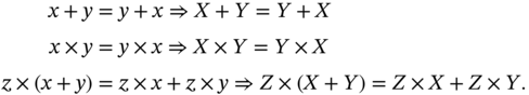
In view of this theorem, we then have the following corollary that gives a new reformulation of the dependency relation.
This corollary assures an important and peculiar property of universal interval arithmetic: when a real‐valued function is translated into the corresponding universal function, the semantic of functional dependence is completely conserved, and we have the equivalence
Accordingly, a universal ![]() ‐ary predicate is characterized as follows.
‐ary predicate is characterized as follows.
For instance, let ![]() be
be ![]() . Then
. Then
Combining Theorem 10.19 with Theorem 10.10, we obtain the following result that establishes the relation between a universal rational function and its corresponding classical interval function.
Thus, by virtue of our formalization of the notion of interval dependency (Definition 10.20), the theory of universal intervals, unlike the classical interval theory and its alternates, copes with all possible cases of functional dependence between interval variables and hence the name “universal interval arithmetic.” This makes our construction differ fundamentally from the interval theories discussed in the previous sections.
10.8.2 The Arithmetic of Universal Intervals
On grounds of the results obtained in Section 10.8.1, we are now ready to formally construct the arithmetic of the theory ![]() of universal interval numbers. We begin by establishing some theorems concerning the universal interval operations. Then, we provide some numerical examples to illustrate how interval dependencies are fully addressed by universal interval arithmetic.
of universal interval numbers. We begin by establishing some theorems concerning the universal interval operations. Then, we provide some numerical examples to illustrate how interval dependencies are fully addressed by universal interval arithmetic.
In particular, Theorem 10.19, plus Definitions 10.28 and 10.29, implies the following four easily derivable results.
These results, along with Theorem 10.20, express an important fact of our development: for the case when ![]() , the value of a universal interval operation is the same as that of the corresponding classical interval operation, that is,
, the value of a universal interval operation is the same as that of the corresponding classical interval operation, that is, ![]() ; and for the case when
; and for the case when ![]() , a universal interval operation gives a different value, according to the dependency function
, a universal interval operation gives a different value, according to the dependency function ![]() . This is why universal interval arithmetic copes with all possible cases of interval dependency. In order to clarify the matters, let, for example,
. This is why universal interval arithmetic copes with all possible cases of interval dependency. In order to clarify the matters, let, for example, ![]() be a real sentence that takes the prenex form
be a real sentence that takes the prenex form
The Skolem equivalent form of ![]() is
is
Such a sentence, as we proved in Section 10.7.2, is not expressible by the partial parametric operations, and its dependency relations are not considered by the classical interval operations. In contrast, the sentence ![]() can be evaluated in universal interval arithmetic, with its dependency relations are completely coped with. Therefore, it comes as a matter of fact that the theory of universal intervals is completely compatible with the semantic of real arithmetic. That is, any sentence of real arithmetic can be translated into a semantically equivalent sentence of universal interval arithmetic.
can be evaluated in universal interval arithmetic, with its dependency relations are completely coped with. Therefore, it comes as a matter of fact that the theory of universal intervals is completely compatible with the semantic of real arithmetic. That is, any sentence of real arithmetic can be translated into a semantically equivalent sentence of universal interval arithmetic.
To complete our construction of universal interval arithmetic, we next define the total operation of “subtraction,” and the partial operations of “division” and “integer exponentiation,” for universal interval numbers.
In view of this definition, we have, as an immediate consequence, the following theorem that prescribes the properties of integer exponents of universal interval numbers.
Accordingly, we also have the following easy‐deducible corollary.
To clarify how interval dependencies are fully addressed by the universal interval operations, in a way which is completely compatible with the semantic of real arithmetic, consider the real‐valued square function
with ![]() and
and ![]() . The value of the corresponding classical interval function, according to Theorem 10.2, is given by
. The value of the corresponding classical interval function, according to Theorem 10.2, is given by
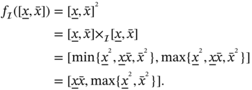
which is not consistent with the fact that a square is always non‐negative. Strictly speaking, the accurate image of the real‐valued function ![]() is a proper subset of the value of the corresponding classical interval function
is a proper subset of the value of the corresponding classical interval function ![]() , that is
, that is
Now, the value of the corresponding universal interval function, according to Theorem 10.22 and Definition 10.34, is given by

which is always non‐negative, and we have the identity
Therefore, unlike classical interval exponentiation, universal exponentiation is completely compatible with the semantic of the real‐valued function ![]() , with
, with ![]() .
.
Therefore, with this construction of the universal interval theory at our disposal, it is not surprising that we can formulate and evaluate interval arithmetic expressions in a way analogous to that of real arithmetic. As a further illustration, let us consider some examples.
The identity ![]() , in the above example, expresses the fact that additive inverses exist in universal interval arithmetic. This fact, along with the fundamental algebraic properties of universal interval arithmetic, shall be established in Section 10.9.
, in the above example, expresses the fact that additive inverses exist in universal interval arithmetic. This fact, along with the fundamental algebraic properties of universal interval arithmetic, shall be established in Section 10.9.
Aside from the important fact that universal interval arithmetic copes with all possible cases of interval dependency, the cornerstone result from the above construction is that each of the universal operations of addition and multiplication, unlike the case with parametric intervals, is a single “total operation” on ![]() , not a “partial operation,” and therefore, we can fix the structures
, not a “partial operation,” and therefore, we can fix the structures ![]() and
and ![]() and study their properties in the standard way. A careful investigation of the algebraic system of universal interval arithmetic is attempted in Section 10.9.
and study their properties in the standard way. A careful investigation of the algebraic system of universal interval arithmetic is attempted in Section 10.9.
Finally, we close this section by characterizing point operations for universal intervals. A point universal interval operation is an operation whose operands are universal intervals, and whose result is a point universal interval (or, up to isomorphism, a real number). This is made precise in the following definition.
Point operations, for a universal interval number ![]() , are also optimization functions with respect to the argument
, are also optimization functions with respect to the argument ![]() and have the same results as in classical interval arithmetic. Next, we define some of the point operations for universal interval numbers.
and have the same results as in classical interval arithmetic. Next, we define some of the point operations for universal interval numbers.
- Width:
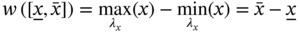 .
. - Radius:
 .
. - Midpoint:
 .
. - Absolute value:
 .
. - Distance:
 .
.
Obviously, for two point universal intervals ![]() and
and ![]() , the universal distance operation reduces to the usual distance operation on the reals. That is
, the universal distance operation reduces to the usual distance operation on the reals. That is
It is also straightforward to prove that the universal distance induces a metric space ![]() on the set
on the set ![]() of universal intervals. The importance of this result is that starting from the distance function for universal intervals, the induced metric space is a generalization of the standard metric space of real numbers. Thus, the notions of a sequence, convergence, continuity, and a limit are readily definable for universal intervals in the standard way. These notions give rise to what we may call a “measure theory for universal intervals.”
of universal intervals. The importance of this result is that starting from the distance function for universal intervals, the induced metric space is a generalization of the standard metric space of real numbers. Thus, the notions of a sequence, convergence, continuity, and a limit are readily definable for universal intervals in the standard way. These notions give rise to what we may call a “measure theory for universal intervals.”
10.9 The S‐Field Algebra of Universal Intervals
We shall now make use of the part of the theory developed in Section 10.8 to in‐depth investigate the algebraic system of universal intervals. In our definition of a universal interval number, the properties of real numbers are naturally assumed in advance.
Let us first mention that as variants of the proofs presented in this section, most of the identities of universal interval arithmetic can be established from the corresponding identities of real arithmetic. This fact is immediately entailed by Theorem 10.19.
In addition, by virtue of Theorems 10.21 –10.24, along with Theorem 10.20, if ![]() , then the result of a universal interval operation is the same as that of the corresponding classical interval operation, that is,
, then the result of a universal interval operation is the same as that of the corresponding classical interval operation, that is, ![]() . This implies that the algebra of universal interval arithmetic will differ from that of classical interval arithmetic for only when
. This implies that the algebra of universal interval arithmetic will differ from that of classical interval arithmetic for only when ![]() . Accordingly, in the proofs of this section, we shall consider only the case when
. Accordingly, in the proofs of this section, we shall consider only the case when ![]() . Moreover, for brevity, and without loss of generality, we shall assume that
. Moreover, for brevity, and without loss of generality, we shall assume that
Our first results of this section, concerning the isomorphism properties, follow immediately from this fact, plus the isomorphism theorem for classical intervals.
That is, up to isomorphism, the algebra of point universal intervals, endowed with Moore's ordering ![]() , is structurally identical to the ordered field of real numbers.
, is structurally identical to the ordered field of real numbers.
That is, universal interval arithmetic extends classical interval arithmetic in the sense that if it is the case when ![]() , then the algebra of the universal interval theory is equivalent to that of the classical interval theory.
, then the algebra of the universal interval theory is equivalent to that of the classical interval theory.
An important theorem we shall now prove is the inclusion monotonicity theorem for universal intervals, which asserts that the inclusion relation is compatible with the algebraic operations on the set ![]() of universal interval numbers.
of universal interval numbers.
Analogously to classical intervals, from the fact that ![]() , the membership monotonicity statements
, the membership monotonicity statements ![]() and
and ![]() are derivable.
are derivable.
Now, we turn to investigate the algebra of universal interval arithmetic. With the help of the results obtained in Section 10.8, we next deduce the fundamental algebraic properties of the universal interval operations.
In a manner analogous to the proof of Theorem 10.29, the next two theorems concerning identity elements are easily provable.
Hereafter, in all the succeeding theorems, and if not otherwise stated, it should be understood that any two interval variables ![]() and
and ![]() can be dependent or independent. The proofs for the case when
can be dependent or independent. The proofs for the case when ![]() and
and ![]() are dependent can be simply obtained, in a manner analogous to the preceding theorems, by employing the equivalence
are dependent can be simply obtained, in a manner analogous to the preceding theorems, by employing the equivalence ![]() . The trivial case of dependence by identity
. The trivial case of dependence by identity ![]() is obvious.
is obvious.
In contrast to the case for addition, and analogously to the classical interval theory, the following theorem asserts that multiplication is not always cancellative22 in ![]() .
.
An important property peculiar to the theory of universal intervals is that unlike classical interval arithmetic, universal interval arithmetic has inverse elements for addition and multiplication. This property figures in the following two theorems.
The result formulated in the following theorem establishes the additive and multiplicative properties of point universal intervals.
In consequence of this theorem and Theorem 10.29, the following important property of the algebra of universal intervals is easily derivable.
Thus, like the algebra of real numbers, the algebra of universal intervals has no nonzero zero divisors, that is for each ![]() , there is no
, there is no ![]() such that the identity
such that the identity ![]() holds.
holds.
Now, we turn to the very desirable algebraic property of distributivity. Distributivity of universal interval arithmetic is established in the next theorem.
Thus, in contrast to the classical interval theory and its present alternates, universal interval arithmetic does satisfy the distributive law.
We shall now make use of the preceding results to prove the following theorem about the algebraic system of universal interval arithmetic.
A field structure ![]() is an integral domain in which every element
is an integral domain in which every element ![]() has a multiplicative inverse. The difference between the field structure and the structure of universal intervals is that for the universal interval algebra, we have the condition
has a multiplicative inverse. The difference between the field structure and the structure of universal intervals is that for the universal interval algebra, we have the condition ![]() instead of
instead of ![]() . Such an algebraic structure is not usual in mathematics, and it emerges from the fact that the elements of the universe set of the universal interval algebra are themselves sets (interval numbers). Therefore, to make an explicit stipulation about this new type of algebraic property, it is very convenient to define a new type of algebraic structure, the set‐valued field (or the S‐field), that extends the ordinary field structure to the case when elements of the universe set are themselves sets.
. Such an algebraic structure is not usual in mathematics, and it emerges from the fact that the elements of the universe set of the universal interval algebra are themselves sets (interval numbers). Therefore, to make an explicit stipulation about this new type of algebraic property, it is very convenient to define a new type of algebraic structure, the set‐valued field (or the S‐field), that extends the ordinary field structure to the case when elements of the universe set are themselves sets.
In view of this definition and Theorem 10.41, the following result can then be concluded.
Finally, an important immediate result that the preceding theorem implies is the following.
Universal intervals thus are S‐numbers, and therefore we, can talk of “universal interval numbers.”
In conclusion, unlike classical interval arithmetic and its present alternates, universal intervals have additive inverses, multiplicative inverses, and satisfy the property of distributivity. By virtue of the algebraic properties proved in this section, universal interval arithmetic possesses a rich S‐field algebra, which extends the ordinary field structure of real numbers, and therefore, we do not have to sacrifice the useful properties of ordinary arithmetic. In addition, with our formalization of the notion of interval dependency at disposal (see Section 10.5.2), universal interval operations are defined such that they exhibit a uniform approach applicable to all cases of interval dependency. Therefore, on comparing the universal interval theory with other theories of intervals, the main advantage that lies with universal interval arithmetic, over all other theories of intervals, is that the theory of universal intervals is completely compatible with the semantic of real arithmetic. That is, any sentence of real arithmetic can be translated into a semantically equivalent sentence of universal interval arithmetic, without loss of dependency information.
10.10 Guaranteed Bounds or Best Approximation or Both?
In some practical situations, some overestimation can be beneficial and important. There are two different problems: getting guaranteed bounds of an exact value and computing an approximation of the value. The two problems are very different. In robotics and control applications, for example, it is important to have guaranteed inclusions of the exact values in order to guarantee stability under uncertainty.
An interval theory is theoretically exact if interval dependencies are fully addressed by its algebraic system, and the accurate results can be symbolically obtained. If an interval theory is theoretically exact, we cannot always have computational guaranteed bounds without proper outward rounding because of the limitations of floating point arithmetic. As an example, the classical interval theory is partially exact if the computed terms are dependency‐free, as for instance, the image of the function ![]() , with
, with ![]() and
and ![]() being functionally independent. We cannot always have guaranteed bounds for the image of
being functionally independent. We cannot always have guaranteed bounds for the image of ![]() , without applying outward rounding. Provided that the universal interval theory is theoretically exact and its algebraic operations are theoretically overestimation‐free, we can get the best guaranteed inclusions by applying a proper outward rounding.
, without applying outward rounding. Provided that the universal interval theory is theoretically exact and its algebraic operations are theoretically overestimation‐free, we can get the best guaranteed inclusions by applying a proper outward rounding.
One issue is that to evaluate a universal interval expression, the minimization and maximization should usually be applied to the whole corresponding real expression, in order not to lose the dependency information. If the problem is too large and the optimization is computationally too costly, we may have to deviate from the theoretical construction of the theory by dividing the optimizational problem and hence losing some dependency information. For example, in the interval expression
we have to apply optimization to the real expression ![]() as a whole to get the accurate result. Optimizing each of the products
as a whole to get the accurate result. Optimizing each of the products ![]() and
and ![]() separately, and then summing the results for the individual optimizations, we shall, with this departure from the theoretical construction, lose the dependency information for
separately, and then summing the results for the individual optimizations, we shall, with this departure from the theoretical construction, lose the dependency information for ![]() .
.
An approach we can use for overcoming this issue is to slightly alter our construction of the theory of universal intervals by representing an interval by a 3‐tuple ![]() called a “triple interval,” where the third “slot”
called a “triple interval,” where the third “slot” ![]() , that we may call the “dependency characterizer,” is a symbolic variable used to keep the dependency information for
, that we may call the “dependency characterizer,” is a symbolic variable used to keep the dependency information for ![]() , as long as there is a live accessible value that uses it. The idea is not to lose the dependency information, during a series of calculations, after evaluating separately an intermediate interval expression, such that after evaluating a function
, as long as there is a live accessible value that uses it. The idea is not to lose the dependency information, during a series of calculations, after evaluating separately an intermediate interval expression, such that after evaluating a function
the third slot ![]() of the resulting interval keeps the dependency information, and a problem which is computationally too costly can be divided into smaller problems without losing the dependency information. Now, we can rewrite the dependency and identity between two universal triple intervals
of the resulting interval keeps the dependency information, and a problem which is computationally too costly can be divided into smaller problems without losing the dependency information. Now, we can rewrite the dependency and identity between two universal triple intervals ![]() and
and ![]() , respectively, as
, respectively, as

Triple interval representations are used, with the classical interval operations, to evaluate the particular interval expressions ![]() and
and ![]() as, respectively,
as, respectively, ![]() and
and ![]() . Although it is limited to such a dependence by identity, examples of this usage can be found in algorithmic algebra and artificial intelligence and are successfully and neatly implementable in symbolic languages (computer algebra systems), automated theorem provers, and numeric languages (see, e.g. [75,76], and [69]). The implementation idea is based on constructing an “interval data structure” with three slots, rather than the usual representation of an interval as a “pair.” In symbolic languages, the “dependency slots” are added to a sequence or a list type. In numerical languages, a variable name is constructed for each newly added dependency slot and a counter incremented (there is a convenient mechanism that is built‐in to “Lisp” for this purpose, a “weak hash table”). The dependency information can also be inherited in any object‐oriented language. As we (humans) ordinarily do not need to see the extra slot, programs ordinarily will not display it in the computer output (see [75]).
. Although it is limited to such a dependence by identity, examples of this usage can be found in algorithmic algebra and artificial intelligence and are successfully and neatly implementable in symbolic languages (computer algebra systems), automated theorem provers, and numeric languages (see, e.g. [75,76], and [69]). The implementation idea is based on constructing an “interval data structure” with three slots, rather than the usual representation of an interval as a “pair.” In symbolic languages, the “dependency slots” are added to a sequence or a list type. In numerical languages, a variable name is constructed for each newly added dependency slot and a counter incremented (there is a convenient mechanism that is built‐in to “Lisp” for this purpose, a “weak hash table”). The dependency information can also be inherited in any object‐oriented language. As we (humans) ordinarily do not need to see the extra slot, programs ordinarily will not display it in the computer output (see [75]).
The following code fragment shows how to perform the operations
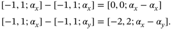
in the computer algebra system “Macsyma” (or “Maxima”) (see, e.g. [77] and [75]).
block([x:interval(-1,1)], x-x)block([x:interval(-1,1),y:interval(-1,1)], x-y)
The idea can be implemented similarly in other symbolic languages such as “SymbolicC++” and “Maple” (see, e.g. [78] and [79]). In automated theorem provers, the 3‐tuple representation of an interval is usually called a “block interval” and the dependency slot is called a “pending identifier” (see, e.g. [69]).
Using the triple interval representation with classical interval arithmetic provides some nice results, such as ![]() , but the outcome is very limited because of the fact that the classical interval operations are not dependence‐aware, and interval dependencies cannot therefore be fully addressed via the classical interval theory (and in fact cannot be fully addressed via the present alternate interval theories as well, and this is why the dependency problem is still persisting). In contrast, using the triple interval representation with universal interval arithmetic shall yield more profound results, namely:
, but the outcome is very limited because of the fact that the classical interval operations are not dependence‐aware, and interval dependencies cannot therefore be fully addressed via the classical interval theory (and in fact cannot be fully addressed via the present alternate interval theories as well, and this is why the dependency problem is still persisting). In contrast, using the triple interval representation with universal interval arithmetic shall yield more profound results, namely:
- Interval dependencies are fully addressed by the universal interval operations, and the accurate result can be computationally obtained, if the problem under concern is not computationally too costly.
- If the problem under concern is computationally too costly (such as an engineering problem with a large number of constrained variables); the computational cost can be reduced to a minimum by using the triple interval representation to keep the dependency information, and dividing the problem into smaller ones.
- From (1) and (2), the accurate result can be obtained, along with the computational cost reduced to a minimum, by using the triple interval representation with universal interval arithmetic.
- Universal interval arithmetic has a nice S‐field algebra, which extends the ordinary field structure of real numbers.
- With universal interval arithmetic equipped with proper outward rounding, we can have reasonable guaranteed bounds of the exact values whenever needed.
Supplementary Materials
To reproduce the results of the calculations in this chapter, latest version of InCLosure is available for free download via https://doi.org/10.5281/zenodo.2702404 or from the first author's website at: http://scholar.cu.edu.eg/henddawood/software/InCLosure. An InCLosure input file and its corresponding output containing, respectively, the code and results of the examples are also available as a supplementary material to this chapter, via http://doi.org/10.5281/zenodo.3236736.
Acknowledgments
The authors would like to thank Prof. Nefertiti Megahed for her advices that greatly contributed to polishing this text and for all the discussions we have had on the subject. We would like also to acknowledge Prof. Snehashish Chakraverty, the editor of this book, for his patience and constructive comments, and for his outstanding help with this chapter. Finally, it is a pleasure to acknowledge the courtesy and substantial help which we have received from the staff of Wiley & Sons at all stages of writing this text.
References
- 1 Dawood, H. (2014). Interval mathematics as a potential weapon against uncertainty. In: Mathematics of Uncertainty Modeling in the Analysis of Engineering and Science Problems, Chapter 1, S. Chakraverty, 1–38. Hershey, PA: IGI Global.ISBN: 978‐1‐4666‐4991‐0. http://dx.doi.org/10.4018/978-1-4666-4991-0.ch001.
- 2 Kosheleva, O. and Kreinovich, V. (2019). Physics Need for Interval Uncertainty and How it Explains Why Physical Space is (at least) 3‐Dimensional. Technical Report UTEP‐CS‐19‐05. University of Texas at El Paso.
- 3 Heath, T.L. (ed.) (2009). The Works of Archimedes: Edited in Modern Notation with Introductory Chapters. Cambridge: Cambridge University Press. https://doi.org/10.1017/CBO9780511695124.
- 4 Moore, R.E (1959). Automatic Error Analysis in Digital Computation. Technical Report LMSD‐48421. Palo Alto, CA: Lockheed Missiles and Space Company, Lockheed Corporation.
- 5 Burkill, J.C. (1924). Functions of intervals. Proceedings of the London Mathematical Society 2 (1): 275–310.
- 6 Young, R.C. (1931). The algebra of many‐valued quantities. Mathematische Annalen 104: 260–290.
- 7 Dwyer, P.S. (1951). Linear Computations. New York: Chapman & Hall.
- 8 Sunaga, T. (1958). Theory of an interval algebra and its application to numerical analysis. RAAG Memoirs 2: 29–46.
- 9 Dawood, H. (2012). Interval mathematics: foundations, algebraic structures, and applications. Master's thesis. Giza: Department of Mathematics, Faculty of Science, Cairo University. http://dx.doi.org/10.13140/RG.2.2.24252.13449.
- 10 Fu, C., Liu, Y., and Xiao, Z. (2019). Interval differential evolution with dimension‐reduction interval analysis method for uncertain optimization problems. Applied Mathematical Modelling 69: 441–452.
- 11 Kreinovich, V. and Shary, S.P. (2016). Interval methods for data fitting under uncertainty: a probabilistic treatment. Reliable Computing 23: 105–141.
- 12 Moore, R.E., Kearfott, R.B., and Cloud, M.J. (2009). Introduction to Interval Analysis. SIAM.
- 13 Rump, S.M. (1999). INTLAB–INTerval LABoratory. In: Developments in Reliable Computing (ed. T. Csendes), 77–104. Dordrecht: Kluwer Academic Publishers.
- 14 Chevillard, S., Joldes, M., and Lauter, C. (2010). Sollya: an environment for the development of numerical codes. In: Mathematical Software ‐ ICMS 2010, Lecture Notes in Computer Science, vol. 6327 (ed. K. Fukuda, J. van der Hoeven, M. Joswig, and N. Takayama), 28–31. Heidelberg: Springer‐Verlag.
- 15 Dawood, H. (2018). InCLosure (Interval enCLosure)–A language and environment for reliable scientific computing. Computer Software, Version 2.0. Giza, Egypt: Department of Mathematics, Faculty of Science, Cairo University. https://doi.org/10.5281/zenodo.2757278. InCLosure Support: http://scholar.cu.edu.eg/henddawood/software/InCLosure.
- 16 Melquiond, G. (2008). Proving bounds on real‐valued functions with computations. In: International Joint Conference on Automated Reasoning IJCAR, Lecture Notes in Artificial Intelligence, vol. 5195 (ed. A. Armando, P. Baumgartner, and G. Dowek), 2–17. Springer‐Verlag. https://doi.org/10.1007/978-3-540-71070-7_2.
- 17 Dawood, H. (2011). Theories of Interval Arithmetic: Mathematical Foundations and Applications. Saarbrücken: LAP Lambert Academic Publishing. ISBN:978‐3‐8465‐0154‐2.
- 18 Dawood, H. (2019). On some algebraic and order‐theoretic aspects of machine interval arithmetic. Online Mathematics Journal (OMJ) 1 (2): 1–13. http://doi.org/10.5281/zenodo.2656089.
- 19 Kolev, L.V. (1993). Interval Methods for Circuit Analysis. World Scientific Publishing Company.
- 20 Kulisch, U.W. (2008). Computer Arithmetic and Validity: Theory, Implementation, and Applications. Walter de Gruyter.
- 21 Muller, J.‐M., Brisebarre, N., De Dinechin, F. et al. (2009). Handbook of Floating‐Point Arithmetic, 1e. Boston, MA: Birkhäuser.
- 22 IEEE 1788 Committee (2015). IEEE Standard for Interval Arithmetic. IEEE Std 1788‐2015, pp. 1–97. https://doi.org/10.1109/IEEESTD.2015.7140721. https://ieeexplore.ieee.org/document/7140721.
- 23 Barnes, D.W. and Mack, J.M. (1975). An Algebraic Introduction to Mathematical Logic, 1e. Springer‐Verlag.
- 24 Dawood, H. and Dawood, Y. (2013). Logical Aspects of Interval Dependency. Technical Report CU‐Math‐2013‐03‐LAID. Department of Mathematics, Faculty of Science, Cairo University.
- 25 Dawood, H. and Dawood, Y. (2014). On Some Order‐Theoretic Aspects of Interval Algebras. Technical Report CU‐Math‐2014‐06‐OTAIA. Department of Mathematics, Faculty of Science, Cairo University.
- 26 Dawood, H. and Dawood, Y. (2017). Investigations Into a Formalized Theory of Interval Differentiation. Technical Report CU‐Math‐2017‐03‐IFTID. Department of Mathematics, Faculty of Science, Cairo University.
- 27 Dawood, H. and Dawood, Y. (2019). A logical formalization of the notion of interval dependency: towards reliable intervalizations of quantifiable uncertainties. Online Mathematics Journal 1 (3). http://doi.org/10.5281/zenodo.3234184.
- 28 Menini, C. and Van Oystaeyen, F. (2004). Abstract Algebra: A Comprehensive Treatment, 1e. CRC Press.
- 29 (a)Cantor, G. (1897). Beitrage zur begrundung der transfiniten mengenlehre II. Mathematische Annalen 49: 207–246;(b) Translated with introduction and commentary by Jourdain, P.E.B. (1955). Contributions to the Founding of the Theory of Transfinite Numbers. New York: Dover Publications.
- 30 Amer, M.A. (1989). First order logic with empty structures. Studia Logica 48 (2): 169–177.
- 31 Suppes, P. (1972). Axiomatic Set Theory. New York: Dover Publications.
- 32 Tarski, A. (1994). Introduction to Logic and to the Methodology of the Deductive Sciences, 4e. New York: Oxford University Press. translated from Polish by Olaf Helmer.
- 33 Mostowski, A. (1951). On the rules of proof in the pure functional calculus of the first order. The Journal of Symbolic Logic 16 (2): 107–111.
- 34 Van Orman Quine, W. (1954). Quantification and the empty domain. The Journal of Symbolic Logic 19 (3): 177–179.
- 35 Hintikka, J. (1959). Existential presuppositions and existential commitments. The Journal of Philosophy 56 (3): 125–137.
- 36 Corcoran, J. (1980). Categoricity. History and Philosophy of Logic 1 (1): 187–207. https://doi.org/10.1080/01445348008837010.
- 37 van Hoorn, W.G. and van Rootselaar, B. (1967). Fundamental notions in the theory of seminearrings. Compositio Mathematica 18 (1–2): 65–78.
- 38 Pilz, G. (1983). Near‐Rings: The Theory and its Applications, North‐Holland Mathematics Studies, vol. 23. North‐Holland Publishing Company.
- 39 Clay, J.R. (1992). Nearrings: Geneses and Applications. Oxford University Press.
- 40 Hansen, E.R. (1975). A generalized interval arithmetic. In: Interval Mathematics, Lecture Notes in Computer Science, vol. 29. (ed. Karl L. E. Nickel), 7–18. Springer‐Verlag.
- 41 Gardenyes, E., Mielgo, H., and Trepat, A. (1985). Modal intervals: reason and ground semantics. In: Interval Mathematics, Lecture Notes in Computer Science, vol. 212. (ed. Karl L. E. Nickel), 27–35. Springer‐Verlag.
- 42 Markov, S.M. (1995). On directed interval arithmetic and its applications. Journal of Universal Computer Science 1 (7): 514–526.
- 43 Lodwick, W.A. (1999). Constrained Interval Arithmetic. Technical Report 138. Denver: University of Colorado at Denver, Center for Computational Mathematics.
- 44 Dawood, H. and Dawood, Y. (2016). Interval Algerbras: A Formalized Treatment. Technical Report CU‐Math‐2016‐06‐IAFT. Department of Mathematics, Faculty of Science, Cairo University.
- 45 Dawood, H. and Dawood, Y. (2013). A Dependency‐Aware Interval Algebra. Technical Report CU‐Math‐2013‐09‐DAIA. Department of Mathematics, Faculty of Science, Cairo University.
- 46 Shayer, S. (1965). Interval Arithmetic with Some Applications for Digital Computers. Technical Report LMSD‐5136512. Palo Alto, CA: Lockheed Missiles and Space Company, Lockheed Corporation.
- 47 Dawood, H. and Dawood, Y. (2010). On the Metamathematics of the Theory of Interval Numbers. Technical Report CU‐Math‐2010‐06‐MTIN. Giza: Department of Mathematics, Faculty of Science, Cairo University.
- 48 Rokne, J. and Ratschek, H. (1984). Computer Methods for the Range of Functions. Ellis Horwood Publications.
- 49 Euler, L. (2000). Foundations of Differential Calculus. Springer‐Verlag.
- 50 Lobachevskii, N.I. (1951). Complete Works 5. Moscow‐Leningrad.
- 51 Armstrong, W.W. (1974). Dependency structures of data base relationships. In: Proceedings of IFIP Congress, 580–583.
- 52 Hintikka, J. (1996). The Principles of Mathematics Revisited. Cambridge University Press.
- 53 Vaananen, J. (2007). Dependence Logic: A New Approach to Independence Friendly Logic. Cambridge University Press.
- 54 Skolem, T.A. (1920). Logisch‐kombinatorische untersuchungen über die erfüllbarkeit oder beweisbarkeit mathematischer satze nebst einem theoreme über dichte mengen. Skrifter utgit av Videnskabsselskapet i Kristiania, I. Matematisk‐Naturvidenskabelig Klasse No. 4, pp. 1–36. Translated from Norwegian as “Logico‐combinatorial investigations on the satisfiability or provability of mathematical propositions: a simplified proof of a theorem by Loewenheim” by Stefan Bauer‐Mengelberg.
- 55 Feferman, S. (2006). What kind of logic is independence‐friendly logic? In The Philosophy of Jaakko Hintikka, Library of Living Philosophers, vol. 30 (ed. R.E. Auxier and L.E. Hahn), 453–469. Open Court Publishing Company.
- 56 Chen, G. and Pham, T.T. (2000). Introduction to Fuzzy Sets, Fuzzy Logic, and Fuzzy Control Systems, 1e, CRC Press.
- 57 Tarski, A. (1951). A Decision Method for Elementary Algebra and Geometry, 2e. University of California Press.
- 58 Basu, S., Pollack, R., and Roy, M.‐F. (2003). Algorithms in Real Algebraic Geometry, 1e. Springer‐Verlag.
- 59 Collins, G.E. (1975). Quantifier elimination for the elementary theory of real closed fields by cylindrical algebraic decomposition. In: Automata Theory and Formal Languages 2nd GI Conference Kaiserslautern, Lecture Notes in Computer Science, vol. 33. (ed. H. Brakhage), 134–183. Springer‐Verlag.
- 60 McCallum, S. (2001). On propagation of equational constraints in cad‐based quantifier elimination. In: Proceedings of the International Symposium on Symbolic and Algebraic Computation, 223–231.
- 61 Corcoran, J. and Ramnauth, A. (2013). Equality and identity. Bulletin of Symbolic Logic 19 (3): 255–256.
- 62 Gaganov, A.A. (1985). Computational complexity of the range of the polynomial in several variables. Cybernetics 21: 418–421.
- 63 Kreinovich, V. (2008). Interval computations as an important part of granular computing: an introduction. In: Handbook of Granular Computing, Chapter 1, 1e (ed. W. Pedrycz, A. Skowron, and V. Kreinovich). Wiley‐Interscience. 3–32.
- 64 Moore, R.E. (1966). Interval Analysis. Prentice Hall.
- 65 Moore, R.E. (1979). Methods and Applications of Interval Analysis, SIAM studies in Applied Mathematics, vol. 2. Philadelphia, PA: SIAM.
- 66 Alefeld, G. and Herzberger, J. (1983). Introduction to Interval Computation, 1e. New York: Academic Press.
- 67 Alefeld, G. and Mayer, G. (2000). Interval analysis: theory and applications. Journal of Computational and Applied Mathematics 121 (1): 421–464.
- 68 Lodwick, W.A. (2008). Fundamentals of interval analysis and linkages to fuzzy set theory. In: Handbook of Granular Computing, Chapter 3, 1e. W. Pedrycz, A. Skowron, and V. Kreinovich). Wiley‐Interscience. 55–79.
- 69 Pichler, F. (2007). Computer Aided Systems Theory. Springer‐Verlag.
- 70 Cleary, J.G. (1987). Logical arithmetic. Future Computing Systems 2 (2): 125–149.
- 71 Cleary, J.G. (1993). Proving the Existence of Solutions in Logical Arithmetic. Technical report 93/5. Hamilton, New Zealand: University of Waikato, Department of Computer Science.
- 72 Dawood, H. and Dawood, Y. (2019). Parametric intervals: more reliable or foundationally problematic? Online Mathematics Journal 1 (3). http://doi.org/10.5281/zenodo.3234186.
- 73 Elishakoff, I. and Miglis, Y. (2012). Overestimation‐free computational version of interval analysis. International Journal for Computational Methods in Engineering Science and Mechanics 13 (5): 319–328. https://doi.org/10.1080/15502287.2012.683134.
- 74 Piegat, A. and Landowski, M. (2017). Is an interval the right result of arithmetic operations on intervals? International Journal of Applied Mathematics and Computer Science 27 (3): 575–590. https://doi.org/10.1515/amcs-2017-0041.
- 75 Fateman, R.J. (2009). Interval Arithmetic, Extended Numbers and Computer Algebra Systems. University of California at Berkeley.
- 76 Keene, S. (1988). Object‐Oriented Programming in Common Lisp: A Programmer's Guide to CLOS. Addison‐Wesley Publishing Company.
- 77 Chu, D. and Barnes, D.J. (2010). Introduction to Modeling for Biosciences. Springer‐Verlag.
- 78 Robertson, J.S. (1996). Engineering Mathematics with Maple. New York: McGraw‐Hill.
- 79 Tan, K.S., Steeb, W.‐H., and Hardy, Y. (2008). Computer Algebra With Symbolic C++. World Scientific.
Notes
- 1 InCLosure (Interval enCLosure) is a language and environment for reliable scientific computing, which is coded entirely in Lisp. Latest version of InCLosure is available for free download via https://doi.org/10.5281/zenodo.2702404.
- 2 Amer in [30] used the
 ‐th Cartesian power of
  to define empty structures and axiomatized their first‐order theory.
 - 3 First‐order logics with empty structures were first considered by Mostowski [33] and then studied by many logicians (see, e.g. [34,35], and [30]). Such logics are now referred to as free logics.
- 4 The axiom of extensionality asserts that two sets are equal if, and only if, they have precisely the same elements, that is, for any two sets
 and
and  ,
,  .
. - 5 The notions, notations, and abbreviations of this section are indispensable for our mathematical discussion throughout the succeeding sections and hereafter are assumed priori, without further mention.
- 6 A quantification matrix
 is a sequence
  , where
  are variable symbols and each
  is
is  or
or  .
. - 7 A prenex sentence is a sentence of the form
 , where
  is a quantification matrix and
  is a quantifier‐free formula.
 - 8 Skolemization is named after the Norwegian logician Thoralf Skolem (1887–1963), who first presented the notion in [54].
- 9 From the fact that the converse relation
 is always definable, the preimage of a function
  is always definable, regardless of the definability of the inverse function
  .
. - 10 A rational real‐valued function is a function obtained by means of a finite number of the basic real algebraic operations
 and
and  .
. - 11 An algebraic function is a function that satisfies a polynomial equation whose coefficients are polynomials with rational coefficients.
- 12 The CAD algorithm is efficient enough for being one of the most important optimization algorithms of computational real algebraic geometry (see, e.g. [58]).
- 13 The notions of identity and equality are commonly confused and treated as synonyms. However, they are two distinct logical concepts. Despite the fact that equality implies identity in the theory of real numbers, this is not always the case. Two line halves are equal but not identical (one and the same). Every line equals infinitely many other lines, but no line is (identical to) any other line (see [61] and [32]). Identity, which is the most fundamental ingredient of any mathematical theory, is characterized by Leibniz's principle of the identity of indiscernibles, which states that two entities
 and
and  are identical iff any property of
  is also a property of
  and vice versa.
 - 14 In principle, this result is not necessarily applicable to other theories of interval arithmetic (present or future) because each theory has its peculiar set of algorithms, where each algorithm is a sequence of elementary relations and functions of the foundational level of the theory.
- 15 Let
 be a vector space over an ordered field
  . A set
  in
in  is said to be convex iff

- 16 Note that various parametrizations can be employed to characterize a parametric interval. As an instance, Elishakoff and Miglis used a trigonometric parametrization in [73]. Here, we use the simple linear parametrization adopted in [17,72], and [43].
- 17 Although we have many theories of intervals being discussed throughout the text, we always deal with the same set of real closed intervals. However, for legibility and brevity, we shall employ different notations for the set of interval numbers, for example,
 ,
,  ,
,  , and so forth, according to what theory of intervals is being discussed. Therefore, we can write, for instance, the brief expressions “addition on
  ” and “addition on
  ” instead, respectively, of the expressions “classical interval addition” and “parametric interval addition.”
 - 18 http://www.gecode.org/.
- 19 http://sourceforge.net/projects/halppc.
- 20 http://minion.sourceforge.net/.
- 21 A similar result for classical interval arithmetic was proved by Moore, for the restricted case when every variable occurs only once on each side of the identity relation, or, in other words, when all variables are functionally independent (see, e.g. [64,65], and [12]) Moore's result is entailed by Theorem 10.8.
- 22 The cancellative laws for addition and multiplication are also derivable from Theorems 10.36 and 10.37, by the fact that every invertible element is cancellable. The cancellative law for multiplication is also entailed by Theorem 10.39, from the fact that an element is not cancellable for multiplication iff it is a zero divisor.
- 23 An integral domain is a commutative unital ring with no zero divisors.