18
Different Techniques to Solve Monotone Inclusion Problems
Tanmoy Som1, Pankaj Gautam1, Avinash Dixit1, and D. R. Sahu2
1Department of Mathematical Sciences, Indian Institute of Technology (Banaras Hindu University), Varanasi, Uttar Pradesh, 221005, India
2Department of Mathematics, Banaras Hindu University, Varanasi, Uttar Pradesh, 221005, India
18.1 Introduction
Consider a monotone operator ![]() . A point
. A point ![]() is zero of
is zero of ![]() if
if ![]() . The set of all zeros of
. The set of all zeros of ![]() is denoted by “zer(T).” A wide class of problems can be reduced to a fundamental problem of nonlinear analysis is to find a zero of a maximal monotone operator
is denoted by “zer(T).” A wide class of problems can be reduced to a fundamental problem of nonlinear analysis is to find a zero of a maximal monotone operator ![]() in a real Hilbert space
in a real Hilbert space ![]() :
:
A more general problem we can consider here is to find ![]() such that
such that ![]() , for some
, for some ![]() . This problem finds many important application in scientific fields such as signal and image processing [1], inverse problems [2,3], convex optimization [4], and machine learning [5].
. This problem finds many important application in scientific fields such as signal and image processing [1], inverse problems [2,3], convex optimization [4], and machine learning [5].
Suppose ![]() is the gradient of a differentiable convex function
is the gradient of a differentiable convex function ![]() , i.e.
, i.e. ![]() , the most simple approach to solve Problem 18.1 is via gradient projection method, given by
, the most simple approach to solve Problem 18.1 is via gradient projection method, given by
where ![]() are stepsizes. The operator
are stepsizes. The operator ![]() is called as forward–backward and the above scheme is nothing else than classical method of steepest descent.
is called as forward–backward and the above scheme is nothing else than classical method of steepest descent.
In case ![]() is nondifferentiable function, gradient method generalizes to subgradient method, given by
is nondifferentiable function, gradient method generalizes to subgradient method, given by
For a general monotone operator ![]() , the classical approach to solve Problem 18.1 is proximal point method, which converts the maximal monotone operator inclusion problem into a fixed point problem of a firmly nonexpansive mapping via resolvent operator. The proximal point algorithm [6,7] is one of the most influential method to solve Problem 18.1 and has been studied extensively both in theory and practice [8–10]. Proximal point algorithm is given by
, the classical approach to solve Problem 18.1 is proximal point method, which converts the maximal monotone operator inclusion problem into a fixed point problem of a firmly nonexpansive mapping via resolvent operator. The proximal point algorithm [6,7] is one of the most influential method to solve Problem 18.1 and has been studied extensively both in theory and practice [8–10]. Proximal point algorithm is given by
where ![]() is regularization parameter.
is regularization parameter.
The operator ![]() is called resolvent operator, introduced by Moreau [11]. The resolvent operator is also known as a backward operator. This method was further extended to monotone operator by Rockafellar [10]. Rockafeller also studied the weak convergence behavior of proximal point algorithm under some mild assumptions. The aim of this chapter is to study the convergence behavior of proximal point algorithm and its different modified form.
is called resolvent operator, introduced by Moreau [11]. The resolvent operator is also known as a backward operator. This method was further extended to monotone operator by Rockafellar [10]. Rockafeller also studied the weak convergence behavior of proximal point algorithm under some mild assumptions. The aim of this chapter is to study the convergence behavior of proximal point algorithm and its different modified form.
In the Section 18.2, we have discussed some definitions and results used to prove the convergence analysis of algorithms. In Section 18.3, we discussed the convergence behavior of proximal point algorithm. In Section 18.4, we have discussed about the splitting algorithms to solve monotone inclusion problems. Section 18.5 deals with the inertial methods to solve monotone inclusion problems. Numerical example is also shown to compare the convergence speed of different algorithms based on inertial technique.
18.2 Preliminaries
Through this chapter, we will denote the Hilbert space by ![]() .
.
An operator ![]() is said to be uniformly monotone on a subset
is said to be uniformly monotone on a subset ![]() if there exists an increasing function
if there exists an increasing function ![]() vanishing only at 0 such that
vanishing only at 0 such that ![]()
![]()
![]()
![]()
The set of fixed points of function ![]() is denoted by
is denoted by ![]() .
.
18.3 Proximal Point Algorithm
18.4 Splitting Algorithms
In many cases, it is difficult to evaluate the resolvent of operator ![]() . Interestingly, sometimes, it is as difficult as the original problem itself. To overcome this problem, the operator
. Interestingly, sometimes, it is as difficult as the original problem itself. To overcome this problem, the operator ![]() splits into sum of two maximal monotone operators
splits into sum of two maximal monotone operators ![]() and
and ![]() such that resolvent of
such that resolvent of ![]() and
and ![]() are easier to compute than the full resolvent
are easier to compute than the full resolvent ![]() . Based on splitting techniques, many iterative methods has been designed to solve Problem 18.1. Some popular methods are Peaceman–Rachford splitting algorithm [15], Douglas–Rachford splitting algorithm [16], and forward–backward algorithm [17].
. Based on splitting techniques, many iterative methods has been designed to solve Problem 18.1. Some popular methods are Peaceman–Rachford splitting algorithm [15], Douglas–Rachford splitting algorithm [16], and forward–backward algorithm [17].
18.4.1 Douglas–Rachford Splitting Algorithm
Douglas–Rachford splitting algorithm is proposed to solve a general class of monotone inclusion problems, when ![]() and
and ![]() are maximally monotone. Let
are maximally monotone. Let ![]() and
and ![]() be a sequence in [0,2]. Then, algorithm is as given as follows:
be a sequence in [0,2]. Then, algorithm is as given as follows:
The convergence behavior of Douglas–Rachford splitting algorithm can be summarized as follows:
18.4.2 Forward–Backward Algorithm
The splitting method discussed above is complicated, and the simplest one is forward–backward method. The forward–backward algorithm, the composition of forward step with respect to ![]() followed by backward step with respect to
followed by backward step with respect to ![]() , is given by
, is given by
The forward–backward splitting method is studied extensively in [18–20]. For the general monotone operators ![]() and
and ![]() , the weak convergence of Algorithm 18.6 has been studied under some restriction on the step‐size.
, the weak convergence of Algorithm 18.6 has been studied under some restriction on the step‐size.
Passty studied the convergence of forward–backward, which can be summarized as follows.
18.5 Inertial Methods
The classical proximal point algorithm converts the maximal monotone operator inclusion problem into a fixed point problem of firmly nonexpansive mapping via resolvent operators. Consider ![]() and
and ![]() are differentiable functions. The proximal point algorithm can be interpreted as one step discretization method for the ordinary differential equations
are differentiable functions. The proximal point algorithm can be interpreted as one step discretization method for the ordinary differential equations
where ![]() represents the derivative of
represents the derivative of ![]() and
and ![]() is the gradient of
is the gradient of ![]() . The iterative method mentioned above are one step, i.e. the new iteration term depends on only its previous iterate. Multistep methods have been proposed to accelerate the convergence speed of the algorithm, which are discretization of second‐order ordinary differential equation
. The iterative method mentioned above are one step, i.e. the new iteration term depends on only its previous iterate. Multistep methods have been proposed to accelerate the convergence speed of the algorithm, which are discretization of second‐order ordinary differential equation
where ![]() . System 18.9 roughly shows the motion of heavy ball rolling under its own inertia over the graph of
. System 18.9 roughly shows the motion of heavy ball rolling under its own inertia over the graph of ![]() until friction stops it at a stationary point of
until friction stops it at a stationary point of ![]() . Inertial force, friction force, and graving force are the three parameters in System 18.9, that is why the system is named heavy‐ball with friction (HBF) system. The energy function is given by
. Inertial force, friction force, and graving force are the three parameters in System 18.9, that is why the system is named heavy‐ball with friction (HBF) system. The energy function is given by
which is always decreasing with ![]() unless
unless ![]() vanishes. Convexity of
vanishes. Convexity of ![]() insures that trajectory will attain minimum point. The convergence speed of the solution trajectories of the System 18.9 is greater than the System 18.8. Polyak [21] first introduced the multistep method using the property of heavy ball System 18.9 to minimize a convex smooth function
insures that trajectory will attain minimum point. The convergence speed of the solution trajectories of the System 18.9 is greater than the System 18.8. Polyak [21] first introduced the multistep method using the property of heavy ball System 18.9 to minimize a convex smooth function ![]() . Polyak's multistep algorithm was given by
. Polyak's multistep algorithm was given by
where ![]() is a momentum parameter and
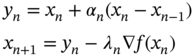
is a momentum parameter and ![]() is a step‐size parameter. It significantly improves the performance of the scheme. Nestrov [22] improves the idea of Polyak by evaluating the gradient at the inertial rather than the previous term. The extrapolation parameter
is a step‐size parameter. It significantly improves the performance of the scheme. Nestrov [22] improves the idea of Polyak by evaluating the gradient at the inertial rather than the previous term. The extrapolation parameter ![]() is chosen to obtain the optimal convergence of the scheme. The scheme is given by
is chosen to obtain the optimal convergence of the scheme. The scheme is given by
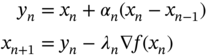
where ![]()
18.5.1 Inertial Proximal Point Algorithm
In 2001, by combining the idea of heavy ball method and proximal point method, Alvarez and Attouch proposed the inertial proximal point algorithm, which can be written as
where ![]() is a set‐valued operator and
is a set‐valued operator and ![]() and
and ![]() are the sequences satisfying some conditions.
are the sequences satisfying some conditions.
18.5.2 Splitting Inertial Proximal Point Algorithm
In 2003, Moudafi and Oliny [23] modified the inertial proximal point algorithm by splitting into maximal monotone operators ![]() and
and ![]() with
with ![]() is single valued, Lipschitz continuous operator and
is single valued, Lipschitz continuous operator and ![]() ‐cocoercive. The proposed algorithm can be given as follows:
‐cocoercive. The proposed algorithm can be given as follows:

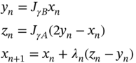
18.5.3 Inertial Douglas–Rachford Splitting Algorithm
This section is dedicated to the formulation of an inertial Douglas–Rachford splitting algorithm, which approaches the set of zeros of the sum of two maximally monotone operators and to the investigation of its convergence properties.
18.5.4 Pock and Lorenz's Variable Metric Forward–Backward Algorithm
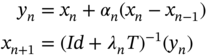
Recently, with the inspiration of Nestrov's accelerated gradient method, Lorenz and Pock [24] proposed a modification of the forward–backward splitting to solve monotone inclusion problems by the sum of a monotone operator whose resolvent is easy to compute and another monotone operator is cocoercive. They have introduced a symmetric, positive definite map ![]() , which is considered as a preconditioner or variable metric. The algorithm can be given as follows:
, which is considered as a preconditioner or variable metric. The algorithm can be given as follows:

where ![]() is an extrapolation factor,
is an extrapolation factor, ![]() is a step‐size parameter.
is a step‐size parameter.
Recently, some inertial iterative algorithms have been proposed, which replaced the condition (iii) of Theorem 18.5 with some mild conditions, which makes the algorithms easy to use for real‐world problems. In 2015, Bot et al. [26] proposed the inertial Mann algorithm for nonexpansive operators and studied the weak convergence in real Hilbert space framework. The inertial Mann algorithm for some initial points ![]() :
:
where ![]() , and
, and ![]() are nonempty, closed, and affine subsets of
are nonempty, closed, and affine subsets of ![]() .
.
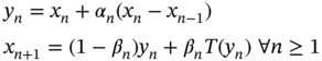
In 2018, Dong et al. [27] proposed a generalized form of inertial Mann algorithm. They included an extra inertial term in inertial Mann algorithm. The algorithm is given as follows:

where ![]() .
.
Convergence analysis can be summarized as follows:
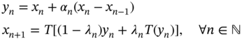
In 2019, Dixit et al. [28] proposed the inertial normal algorithm and studied the weak convergence of the proposed algorithm. The algorithm is given as follows:
18.5.5 Numerical Example
In order to compare the convergence speed of Algorithm 18.27, 18.43, and 18.44 in real Hilbert space ![]() with Euclidean norm, we consider the nonexpansive mapping
with Euclidean norm, we consider the nonexpansive mapping
To show ![]() is nonexpansive mapping, we have for
is nonexpansive mapping, we have for ![]() and
and ![]()
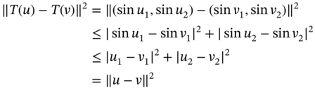
This implies that ![]() , thus
, thus ![]() is nonexpansive. For comparison, we choose the sequences
is nonexpansive. For comparison, we choose the sequences ![]() ,
, ![]() , and
, and ![]() . The convergence behaviors of the algorithms are shown in figure.
. The convergence behaviors of the algorithms are shown in figure.
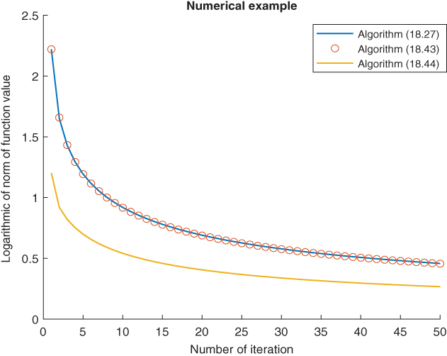
Figure 18.1 Semilog graph between number of iterations and iteration value.
Figure 18.1 shows that the Algorithms 18.27 and 18.43 have nearly same convergence speed but greater than the Mann algorithm. The convergence speed of Algorithm 18.44 is highest. This figure shows the importance of Algorithm 18.44 to calculate the zeros of a nonexpansive mapping.
18.6 Numerical Experiments
Further to compare the convergence speed and accuracy of iterative algorithms 18.27, 18.43, and 18.44 on real‐world problems, we conducted numerical experiments for regression problem on high dimensional datasets that are publicly available. Consider the convex minimization problem given by
where ![]() is a linear map,
is a linear map, ![]() and
and ![]() is sparsity controlling parameter. According to the Karush–Kuhn–Tucker (KKT) condition a point
is sparsity controlling parameter. According to the Karush–Kuhn–Tucker (KKT) condition a point ![]() solves 18.46 if and only if
solves 18.46 if and only if
For any ![]() , Eq. 18.47 becomes
, Eq. 18.47 becomes
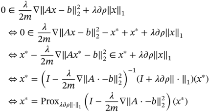
Thus, ![]() minimizes
minimizes ![]() iff
iff ![]() is the fixed point of the operator
is the fixed point of the operator ![]() .
.
Note that here operator ![]() is nonexpansive as
is nonexpansive as ![]() ‐norm is proper lower semicontinuous convex function. Thus, we can apply the Algorithms 18.27, 18.43, and 18.44 to solve the convex minimization problem 18.46.
‐norm is proper lower semicontinuous convex function. Thus, we can apply the Algorithms 18.27, 18.43, and 18.44 to solve the convex minimization problem 18.46.
For numerical experiments, we consider the operator ![]() data matrix having
data matrix having ![]() ‐features and
‐features and ![]() ‐samples, where each
‐samples, where each ![]() is a
is a ![]() ‐dimensional vector
‐dimensional vector ![]() contains
contains ![]() responses. We have taken here datasets from two types of cancer patients: Colon‐cancer dataset and Carcinom dataset.
responses. We have taken here datasets from two types of cancer patients: Colon‐cancer dataset and Carcinom dataset.
(i) Colon‐cancer dataset: Colon cancer is a cancer of large intestine (colon). This dataset is collected from 62 patients having 2000 gene expressions. It contains 40 tumor biopsies from tumors and 22 normal biopsies from healthy parts of the large intestine of the patient.
(i) Carcinom dataset: Carcinoma cancer occurs because of uncontrolled growth of a cell. This dataset contains 174 samples with 9182 features.
For the numerical experiment, we selected ![]() ,
, ![]() , and
, and ![]() . For this choice of
. For this choice of ![]() ,
, ![]() , and
, and ![]() , algorithms satisfies their respective convergence criteria. The sparsity controlling parameter
, algorithms satisfies their respective convergence criteria. The sparsity controlling parameter ![]() is taken as
is taken as ![]() , where
, where ![]() is tuned in the range
is tuned in the range ![]() in the multiple of 0.1. The maximum number of iteration is set to 1000 and to stop the procedure, difference between consecutive iteration should be less than 0.001.
in the multiple of 0.1. The maximum number of iteration is set to 1000 and to stop the procedure, difference between consecutive iteration should be less than 0.001.
In first experiment, we compare the convergence speed of the Algorithms 18.27, 18.43, and 18.44. We plotted the graphs between number of iteration and corresponding function value for each algorithm.
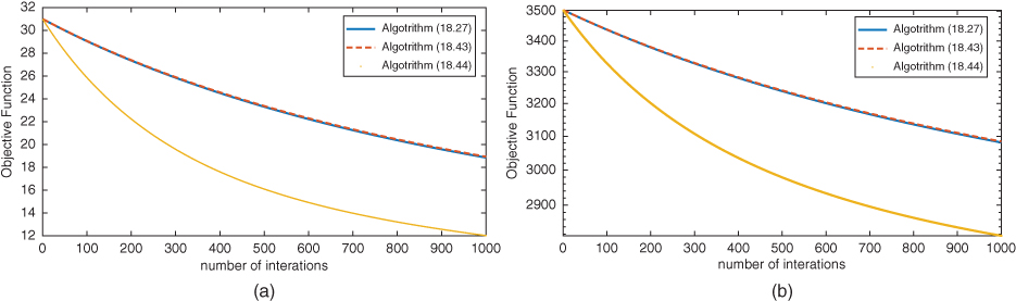
Figure 18.2 The semilog graphs are plotted between number of iteration vs. corresponding objective function value for different datasets. (a) Colon and (b) carcinom.
From Figure 18.2, we can observe that for both the datasets, convergence speed of Algorithm 18.44 is highest and convergence speed of Algorithms 18.27 and 18.43 are nearly the same.
In second experiment, we compare the Algorithms 18.27, 18.43, and 18.44 on the basis of their accuracy for colon dataset and carcinom dataset. We plotted the graphs between number of iterations and corresponding root mean square error (RMSE) value.

Figure 18.3 The semilog graphs are plotted between number of iterations and corresponding root mean square error of the function. (a) Colon and (b) carcinom.
From Figure 18.3, we observe that the RMSE value for Algorithm 18.44 is least while the RMSE values for Algorithms 18.27 and 18.43 are nearly the same.
Thus, we conclude from the observations of Figures 18.2 and 18.3 that Algorithm 18.44 outperforms over Algorithms 18.27 and 18.43.
References
- 1 Byrne, C. (2003). A unified treatment of some iterative algorithms in signal processing and image reconstruction. Inverse Problems 20 (1): 103.
- 2 Combettes, P.L. and Wajs, V.R. (2005). Signal recovery by proximal forward‐backward splitting. Multiscale Modeling and Simulation 4 (4): 1168–1200.
- 3 Daubechies, I., Defrise, M., and De Mol, C. (2004). An iterative thresholding algorithm for linear inverse problems with a sparsity constraint. Communications on Pure and Applied Mathematics: A Journal Issued by the Courant Institute of Mathematical Sciences 57 (11): 1413–1457.
- 4 Bauschke, H.H. and Borwein, J.M. (1996). On projection algorithms for solving convex feasibility problems. SIAM Review 38 (3): 367–426.
- 5 Koh, K., Kim, S.‐J., and Boyd, S. (2007). An interior‐point method for large‐scale l1‐regularized logistic regression. Journal of Machine Learning Research 8: 1519–1555.
- 6 Minty, G.J. (1962). Monotone (nonlinear) operators in Hilbert space. Duke Mathematical Journal 29 (3): 341–346.
- 7 Martinet, B. (1970). Brève communication. Régularisation d'inéquations variationnelles par approximations successives. ESAIM: Mathematical Modelling and Numerical Analysis‐Modélisation Mathématique et Analyse Numérique 4 (R3): 154–158.
- 8 Eckstein, J. and Bertsekas, D.P. (1992). On the Douglas–Rachford splitting method and the proximal point algorithm for maximal monotone operators. Mathematical Programming 55 (1–3): 293–318.
- 9 Güler, O. (1992). New proximal point algorithms for convex minimization. SIAM Journal on Optimization 2 (4): 649–664.
- 10 Rockafellar, R.T. (1976). Monotone operators and the proximal point algorithm. SIAM Journal on Control and Optimization 14 (5): 877–898.
- 11 Moreau, J.‐J. (1965). Proximité et dualité dans un espace Hilbertien. Bulletin de la Société mathématique de France 93: 273–299.
- 12 Bauschke, H.H. and Patrick, L.C. (2011). Convex Analysis and Monotone Operator Theory in Hilbert Spaces, vol. 408. New York: Springer.
- 13 Alvarez, F. and Attouch, H. (2001). An inertial proximal method for maximal monotone operators via discretization of a nonlinear oscillator with damping. Set‐Valued Analysis 9 (1–2): 3–11.
- 14 Alvarez, F (2004). Weak convergence of a relaxed and inertial hybrid projection‐proximal point algorithm for maximal monotone operators in Hilbert space. SIAM Journal on Optimization 14 (3): 773–782.
- 15 Peaceman, D.W. and Rachford, H.H. Jr. (1955). The numerical solution of parabolic and elliptic differential equations. Journal of the Society for Industrial and Applied Mathematics 3 (1): 28–41.
- 16 Douglas, J. and Rachford, H.H. (1956). On the numerical solution of heat conduction problems in two and three space variables. Transactions of the American Mathematical Society 82 (2): 421–439.
- 17 Passty, G.B. (1979). Ergodic convergence to a zero of the sum of monotone operators in Hilbert space. Journal of Mathematical Analysis and Applications 72 (2): 383–390.
- 18 Combettes, P.L. and Wajs V.R. (2005). Signal recovery by proximal forward‐backward splitting. Multiscale Modeling and Simulation 4 (4): 1168–1200.
- 19 Lions, P.‐L. and Mercier, B. (1979). Splitting algorithms for the sum of two nonlinear operators. SIAM Journal on Numerical Analysis 16 (6): 964–979.
- 20 Bauschke, H.H., Matous&c.breve;ková, E., and Reich, S. (2004). Projection and proximal point methods: convergence results and counterexamples. Nonlinear Analysis: Theory Methods & Applications 56 (5): 715–738.
- 21 Polyak, B.T. (1964). Some methods of speeding up the convergence of iteration methods. USSR Computational Mathematics and Mathematical Physics 4 (5): 1–17.
- 22 Nesterov, Y.E. (1983). A method for solving the convex programming problem with convergence rate . Doklady Akademii Nauk SSSR 269: 543–547.
- 23 Moudafi, A. and Oliny, M. (2003). Convergence of a splitting inertial proximal method for monotone operators. Journal of Computational and Applied Mathematics 155 (2): 447–454.
- 24 Lorenz, D.A. and Pock, T. (2015). An inertial forward‐backward algorithm for monotone inclusions. Journal of Mathematical Imaging and Vision 51 (2): 311–325.
- 25 Alvarez, F. and Attouch, H. (2001). An inertial proximal method for maximal monotone operators via discretization of a nonlinear oscillator with damping. Set‐Valued Analysis 9 (1–2): 3–11.
- 26 Bot, R.I., Csetnek, E.R., and Hendrich, C. (2015). Inertial Douglas–Rachford splitting for monotone inclusion problems. Applied Mathematics and Computation 256: 472–487.
- 27 Dong, Q.‐L., Cho, Y.J., and Rassias, T.M. (2018). General inertial Mann algorithms and their convergence analysis for nonexpansive mappings. In: Applications of Nonlinear Analysis (ed. T.M. Rassias), 175–191. Cham: Springer.
- 28 Dixit, A., Sahu, D.R., Singh, A.K., and Som, T. (2019). Application of a new accelerated algorithm to regression problems. Soft Computing 24 (2): 1–14.