
CHAPTER 6
Factor Investing
6.1. INTRODUCTION
Factor investing is a popular way to gain excess returns on top of market returns in the long run while offering a variety of different investment options. In general, a factor can be thought of as any characteristic relating to a group of securities that is important in explaining their returns. Alternative data sources can be used to devise or anticipate investment factors and hence, in principle, a strategy that can outperform other passive investing schemes, as we will show in the next chapters. In this chapter we will summarize the foundations of factor investing and point to how alternative data can be used to create or enhance factors. Nevertheless, we must say that factor investing is not the only way to make use of alternative data. Indeed, in Chapters 1 and 2, we noted that discretionary investors could also incorporate alternative data in their framework. They could, for example, use one-off surveys to confirm/disconfirm their belief about a position they hold.
6.1.1. The CAPM
Using Markowitz's work as their foundation,1 Treynor (1962), Sharpe (1964), Lintner (1965), and Mossin (1966) all independently developed what is now referred to as the Capital Asset Pricing Model (CAPM).
On top of Markowitz's assumptions, the CAPM further assumes that (1) there exists a risk-free rate at which all investors may lend or borrow an infinite amount, and (2) all investors possess homogeneous views on the expected return and volatility of all assets. Under CAPM, all asset returns are explained by the market return plus some random noise specific to each asset and unrelated to any other common factor, in other words the idiosyncratic risk. In terms of expectations this is expressed as:
where ![]() is the return of the asset
is the return of the asset ![]() ,
, ![]() is the return of the market,
is the return of the market, ![]() the risk-free rate, and
the risk-free rate, and ![]() , with
, with ![]() the correlation between the portfolio and the market, and
the correlation between the portfolio and the market, and ![]() and
and ![]() the standard deviations of the portfolio and market returns respectively. Hence the CAPM is a one-factor model where the only factor is the market.
the standard deviations of the portfolio and market returns respectively. Hence the CAPM is a one-factor model where the only factor is the market.
It is important to note that the CAPM can be derived more fundamentally from a two-period equilibrium model2 based on investor optimization, consumption, and market clearing, so its simple form in Equation 6.1 could be misleading as to the depth of the economic theory behind it. Still the assumptions behind it are very simplified and stylized. Nevertheless, it has gained wide popularity and has worked pretty well for a long time.
However, a large amount of empirical evidence has been accumulated showing that it does not describe other sources of return beyond the movements of the market portfolio (Fama and French, 2004). Because of this, many researchers have proposed alternative multifactor models. We discuss some of them here, but before doing so, we will introduce more formally the notion of a factor model. One thing to note in this discussion is that, of course, what we define as the beta, or market factor, is not a “hard” fact, but more a proxy of what a typical market investor's returns would look like. In some assets, a proxy to the market is relatively easy to define; for example, in stocks we might choose S&P 500 while in bonds it might be an index such as the Bloomberg Barclays Global Agg. For other asset classes, like FX, there isn't a widely accepted notion of market index.3
6.2. FACTOR MODELS
Definition: (Factor Model) – Suppose we have a set of ![]() observable random variables,
observable random variables, ![]() . We say that the
. We say that the ![]() follow a factor model if given another set of random variables
follow a factor model if given another set of random variables ![]() , with
, with ![]() , and
, and ![]() , we have that:
, we have that:
where the ![]() ,
, ![]() ,
, ![]() and
and ![]() are independent, that is,
are independent, that is, ![]() , and the matrix
, and the matrix ![]() is non-singular. The
is non-singular. The ![]() are most often associated with asset returns but can be prices or payoffs. Sometimes it is also assumed that
are most often associated with asset returns but can be prices or payoffs. Sometimes it is also assumed that ![]() and, if this is the case, one says that the
and, if this is the case, one says that the ![]() follow a strict factor model.4
follow a strict factor model.4
There are three main types of factors: macroeconomic, statistical, and fundamental (see Connor et al., 2010). Macroeconomic factors can, for example, be surprises in GDP, surprises in inflation, and so on. Statistical factors, on the other hand, are identified through data mining techniques on time series of asset returns. They could be devoid of any economic meaning. Finally, fundamental factors capture stock characteristics, such as industry membership, country membership, valuation ratios, and technical indicators. Some of these factors have become so commonplace that they can often be referred to as beta factors and are the basis of many so-called “smart beta” investing approaches; some particular examples of this can be momentum-based approaches, and indeed we shall discuss such a momentum factor later in this chapter.
Connor (1995) compares the fit of the three types of factor models – macroeconomic, statistical, and fundamental – on the same universe of assets (US equities). He finds that the macroeconomic model performs poorly compared to the other two. This seems intuitive, given that macroeconomic factors are more likely to be suited to macro-based assets, such as equity indices or FX, rather than for trying to explain the behavior of single stocks. While macroeconomic factors do impact stocks as a whole, they are unlikely to be able to explain the idiosyncratic behavior of specific stocks. The fundamental model outperforms the statistical, which at first sight might appear surprising as statistical models are designed to maximize the fit. Connor attributes this to the larger number of factors used in the fundamental model. In fact, the statistical model is focused on the returns dataset only while the fundamental one incorporates extra factors, such as industry identifiers.
According to the type of model and the way we choose to calibrate it, the number of parameters we have to estimate differs, and sometimes having a parsimonious model is highly desirable. Suppose we have time series of length ![]() . Then we will have the following sets of parameters to estimate for each type of model5 (suppose a strict factor model):
. Then we will have the following sets of parameters to estimate for each type of model5 (suppose a strict factor model):
- Statistical: We have to estimate
 6 (time series/cross-sectional regression), which translates into:
(6.3)
6 (time series/cross-sectional regression), which translates into:
(6.3)
parameters, using the
 panel dataset of returns.
 - Macroeconomic: We have to estimate
 (time series regression), which translates into:
(6.4)
(time series regression), which translates into:
(6.4)
parameters, using the
 panel dataset of returns and
  set of macroeconomic factor innovations.
 - Fundamental: We have to estimate
 (cross-sectional regression), which translates into:
(6.5)
(cross-sectional regression), which translates into:
(6.5)
parameters, using the
 panel dataset of returns and
  set of asset characteristics.
For large ![]() the fundamental model has fewer parameters than the other two. However, it uses the most data as the
the fundamental model has fewer parameters than the other two. However, it uses the most data as the ![]() dimensional cross-section of fundamental characteristics is usually larger than the
dimensional cross-section of fundamental characteristics is usually larger than the ![]() dimensional dataset of macroeconomic factors. This means that the fundamental model has more information per parameter in case of large
dimensional dataset of macroeconomic factors. This means that the fundamental model has more information per parameter in case of large ![]() . Compare all three cases to a situation where one has to estimate directly the covariance matrix of the asset returns (i.e. no factor model involved). This means estimating
. Compare all three cases to a situation where one has to estimate directly the covariance matrix of the asset returns (i.e. no factor model involved). This means estimating ![]() parameters, which for large
parameters, which for large ![]() is a number significantly higher that those of the strict factor models we have discussed.
is a number significantly higher that those of the strict factor models we have discussed.
Connor (1995) also experiments with hybrid models, for example, macroeconomic and fundamental. The results show that both statistical and fundamental factors can enrich the macroeconomic model. The opposite is not true in his findings – macroeconomic factors add little to the explanatory power of the statistical and fundamental factors. Miller (2006) shows on a dataset consisting of Japanese equities that at weekly and monthly frequency fundamental models outperform statistical ones. However, he shows that, at daily frequency, a hybrid model of the two can show better performance.
6.2.1. The Arbitrage Pricing Theory
Stephen Ross (1972, 1973, 2013) proposed a purely statistical model to explain asset returns based on the multi-factor formulation of Equation 6.2 without the economic structure behind the CAPM. Using the law of one price in Equation 6.2 and neglecting the error term leads (given it has a mean of zero) to:7
with![]() , that is, the APT imposes a strict factor model on the returns. It is worth noting that, unlike CAPM, APT tells us nothing about what these factors should be or about the sign of each factor's excess return
, that is, the APT imposes a strict factor model on the returns. It is worth noting that, unlike CAPM, APT tells us nothing about what these factors should be or about the sign of each factor's excess return ![]() .8 The number and nature of these factors could potentially vary over time and across markets. As a direct influence of the APT, many new multi-factor models were proposed after its publication. We will now examine the most famous of them – the Fama-French model.
.8 The number and nature of these factors could potentially vary over time and across markets. As a direct influence of the APT, many new multi-factor models were proposed after its publication. We will now examine the most famous of them – the Fama-French model.
6.2.2. The Fama-French 3-Factor Model
Fama and French (Fama and French, 1992) developed a widely accepted model and the most successful one so far. We can say that it belongs to the class of hybrid models based on both macroeconomic (the market) and fundamental factors.
Fama and French showed that the CAPM fails to adequately explain asset returns cross-sectionally for portfolios consisting of small/large stocks, and of portfolios consisting of high/low book-to-market9 ratio stocks. It tends to underestimate returns for small or high-value stocks and overestimate them for big or low-value stocks.10 Fama and French used portfolios based on these ratios and time series regression analysis to show the significance of these factors. More specifically they proposed the following model to explain the returns of the portfolios over the risk-free rate:
where ![]() is the return of portfolio
is the return of portfolio ![]() ,
, ![]() the risk free rate,
the risk free rate, ![]() the market return (calculated as the return on the market cap weighted portfolio of all stocks),
the market return (calculated as the return on the market cap weighted portfolio of all stocks), ![]() the returns of small stocks over big stocks,
the returns of small stocks over big stocks, ![]() returns of high-value stocks over low-value stocks, and
returns of high-value stocks over low-value stocks, and ![]() stochastic error term. The
stochastic error term. The ![]() and
and ![]() are constructed as follows. The stocks universe is partitioned by book-to-market ratio into 3 groups and by market-cap into 2 groups. Then the following further partitions are created as a Cartesian product; that is,
are constructed as follows. The stocks universe is partitioned by book-to-market ratio into 3 groups and by market-cap into 2 groups. Then the following further partitions are created as a Cartesian product; that is, ![]() . Then the following quantities are calculated:
. Then the following quantities are calculated:
in which ![]() and
and ![]() are calculated monthly.
are calculated monthly.
Throughout Fama and French (1992), Fama and French (1993), and Fama and French (1995) it is shown that the Fama-French 3-factor model explains cross-sectional asset returns better than CAPM. In fact, their 3-factor model yields adjusted ![]() above 0.9 for 21 out of 25 examined portfolios. In contrast, by using only CAPM, just 2 out of 25 cases yield such good results (Fama and French, 1993, pp. 19–25).
above 0.9 for 21 out of 25 examined portfolios. In contrast, by using only CAPM, just 2 out of 25 cases yield such good results (Fama and French, 1993, pp. 19–25).
Hence, rather than taking an equilibrium-based approach as the one on which the CAPM is founded, Fama and French based their model on purely empirical findings in the spirit of APT. A lot of explanations have been attempted ever since to understand why these factors fit empirical data so well. Are they proxy for some macroeconomic variables? Although in this way they would be easier to motivate, attempts to explain in this way the ![]() and
and ![]() factors have not been extremely successful. However, research went also in the direction of complementing the
factors have not been extremely successful. However, research went also in the direction of complementing the ![]() and
and ![]() factors with other factors with which their correlation is low. Momentum is such a factor, and this motivated the Carhart model, which we now describe.
factors with other factors with which their correlation is low. Momentum is such a factor, and this motivated the Carhart model, which we now describe.
6.2.3. The Carhart Model
There is empirical evidence that a long portfolio of long-term bad performers and short previous long-term high performers does better than the opposite (see Fama and French, 1996). The performance is calculated over a long period – that is, in the interval ![]() years before the rebalancing date. This may sound intuitive because stocks that have done too well in the past might be overpriced and vice versa. Fama and French, however, manage to explain the outcome of this strategy in terms of their
years before the rebalancing date. This may sound intuitive because stocks that have done too well in the past might be overpriced and vice versa. Fama and French, however, manage to explain the outcome of this strategy in terms of their ![]() factor (i.e. bad performers have higher
factor (i.e. bad performers have higher ![]() ).
).
However, if performance is calculated over the last 12 months – that is, not in the interval ![]() years – the picture is the opposite: good performers tend to continue to perform well and vice versa. This behavior cannot be explained by the Fama-French factors. This led Carhart (see Carhart, 1997) to propose a 4-factor model, which, in addition to the Fama-French factors, includes a momentum factor:
years – the picture is the opposite: good performers tend to continue to perform well and vice versa. This behavior cannot be explained by the Fama-French factors. This led Carhart (see Carhart, 1997) to propose a 4-factor model, which, in addition to the Fama-French factors, includes a momentum factor:
in which ![]() is constructed as the equal-weighted average of stocks with the highest 30% 11-month returns lagged one month minus the equal-weighted average of stocks with the lowest 30% eleven-month returns lagged one month. Carhart proves the significance of this regression on a dataset of funds returns. However, he also shows that after accounting for transaction costs, such a strategy is not necessarily winning. The Fama-French and Carhart models are not the only ones (although the most famous and tested!) that we can use in practice. There is no fundamental reason to believe, though, that the factors they propose are the only viable ones, neither to strictly adopt the sorting approach it is based upon. A more data-mining-based approach, which we will now discuss, is also perfectly justifiable.
is constructed as the equal-weighted average of stocks with the highest 30% 11-month returns lagged one month minus the equal-weighted average of stocks with the lowest 30% eleven-month returns lagged one month. Carhart proves the significance of this regression on a dataset of funds returns. However, he also shows that after accounting for transaction costs, such a strategy is not necessarily winning. The Fama-French and Carhart models are not the only ones (although the most famous and tested!) that we can use in practice. There is no fundamental reason to believe, though, that the factors they propose are the only viable ones, neither to strictly adopt the sorting approach it is based upon. A more data-mining-based approach, which we will now discuss, is also perfectly justifiable.
6.2.4. Other Approaches (Data Mining)
Investors have long been in search of factors that indicate high or low average returns, seeking to construct portfolios based on those. These factors should not necessarily be constructed from the financial statements alone. Indeed, the case for using alternative data is that we can gain something on the top of accounting variables.11
We must note that there are some caveats to a pure data mining approach though. As pointed out by Yan and Zheng (2017), an important debate in the literature is whether the data-mined abnormal returns that can be generated by a strategy are compensation for systematic risk. One example of this is the carry-based factor model, which typically involves sorting assets by their carry (e.g. dividends in stocks). Long positions are taken in higher carry assets, funded by short positions in low carry assets. Typically, those assets with higher levels of carry are also more prone to large drawdowns. Hence, the strategy effectively harvests a risk premium, which is subject to periodic episodes of stress during market turbulence.
While data mining can uncover evidence of market inefficiencies, it is also prone to detecting patterns that are completely spurious and unstable through time. In other words, are we simply fitting to statistical noise? For example, in the case many variables are considered, then by pure chance this could lead to abnormal returns even if these variables do not genuinely have any predictive ability for future stock returns. An important test to perform in this case is whether the uncovered signals are due to sampling variation. Other desirable properties of the factors to be looked for are, for example, persistence over time, large enough variability in returns relative to individual stock volatility, and application to a broad enough subset of stocks within the defined universe (Miller, 2006).
Yan (2017), having first shown in their research that the fundamental-based anomalies they discover are not due to random chance, investigate whether they are consistent with mispricing or risk-based explanations. They conduct three tests for this purpose. We refer the reader to Yan (2017) for details around these tests but what is important to note is that their results indicate that a large number of fundamental factors exhibit genuine predictive ability for future stock returns. That evidence suggests that fundamental-based anomalies are more consistent with mispricing-based explanations.
While some of their factors have been explored in previous studies by other authors, many of the top fundamental signals identified in the Yan (2017) study were new at the time of publication and had received little attention in the prior literature. For example, they find that anomaly variables constructed based on, for example, interest expense, tax loss carry-forward, and selling, general, and administrative expense are highly correlated with future stock returns. They argue that it is reasonable to assume that these variables may predict future stock returns because they contain value-relevant information about future firm performance and the market fails to incorporate this information into stock prices in a timely manner. They conclude that limited attention is a more plausible reason of why investors fail to fully appreciate the information content of the fundamental variables documented in their study. We will leverage the approach and the findings of Yan (2017) later in Chapter 10.
An important test that we could perform is how the newly discovered factors correlate with the Fama-French factors. This will show us whether the former are a proxy for the latter and hence redundant, or whether they indeed contain some additional signals. In the same spirit, Fama and French (1996) analyzed strategies based on factors different from the ![]() and
and ![]() and found that the strategies are mostly explained by their factors, and not purely by the market beta. Indeed, a key point of using alternative data is the hypothesis that by using an unusual dataset we are less likely to find a signal that correlates with existing factors.
and found that the strategies are mostly explained by their factors, and not purely by the market beta. Indeed, a key point of using alternative data is the hypothesis that by using an unusual dataset we are less likely to find a signal that correlates with existing factors.
6.3. THE DIFFERENCE BETWEEN CROSS-SECTIONAL AND TIME SERIES TRADING APPROACHES
Throughout this chapter, the trading rules we have discussed include ranking assets based upon a specific factor. We then take positions in these assets depending on their ranking. In other words, we are constructing cross-sectional trading rules. Hence our position in one asset is impacted by the position in another one. While cross-sectional rules are popular in equities, they can also be found in other asset classes when a factor-driven approach to trading is used, based, for example, on carry, which can be applied to many asset classes including FX. Sometimes these can be used to create market-neutral portfolios or alternatively to adjust the weightings on a long-only portfolio.
This contrasts to purely time-series-driven trading rules, such as those adopted by many managed futures trend-following funds. Typically, they trade futures in various macro-based assets, including sovereign bonds, FX, equity indices, and commodities, as opposed to single stocks. They take long or short positions in a particular future, purely based upon the trend in that asset, which is calculated based on the time series of a specific asset. This contrasts to a cross-sectional approach, where we use some sort of ranking approach across many assets at the same time.
6.4. WHY FACTOR INVESTING?
At this point, it is natural for one to ask what is the empirical evidence of performance when using factor-based strategies? There is some evidence that in good market conditions, indices based on extra factors do tend to outperform a simpler passive approach such as being long a market-cap index. We do of course note that, while such approaches are typically referred to as passive, in practice, such indices do have rebalancing rules associated with them, which tend to favor the larger cap stocks over time. Hence, “passive” strategies might be more active than investors believe.
In bad conditions, however, factor-based strategies can underperform the market (see Ang, 2014). Particular examples of this are those that harvest a risk premium, like carry, as we have noted. In general, however, markets seem to grow and have longer periods of strength than of weakness. In the long run then, it would make sense that market returns occurring in growth periods more than compensate for poor returns occurring during market declines and beat the market index. In fact, this is exactly what we have seen. Since 1973, there have been multiple periods in which factor indices12 have underperformed the market. Overall, however, $1 invested in the MSCI World index from 1973 to 2015 would have risen to $34, whereas $1 invested in their value index would have risen to $49, or to $98 in their momentum index13 (see Authers, 2015). In the long run, then, it seems that the benefits outweigh the costs, at least given the current empirical evidence.
Given the historical evidence of outperformance of these factors over the market, a new type of passive investing has appeared. Rather than investing in the whole market weighted by market cap, investors decided to incorporate these findings by selecting subsets of the market to invest in, based on these factors (factor investing) or using alternative weighting systems to the market cap (smart beta investing). The benefits of these methods are similar to those of passive investing:
- Large investment capacity: Due to investing in indices, the market cap of the chosen investment universe is very large. It would, therefore, take an extreme amount of capital to move the market in some way (i.e. not to be a price taker). This is very attractive to large funds (e.g. pension funds), because many smaller strategies do not scale well when dealing with portfolio values in the high millions/billions.
- Low costs: As these methods are quite simple and can be readily automated, little effort is required to execute them. Thus, costs are low in terms of both factor selection and execution. In the past many of these smart beta strategies were typically only available to investors who allocated to hedge funds while these days variants of these factors are available through lower-cost wrappers such as ETFs.
- Diversification: As these methods are based on index investing, we still experience, given a large enough universe to invest over, a very good level of diversification among stocks.
Clarke et al. (2005) show that, with the addition of factor investment strategies, one can expand the efficient frontier and push/rotate it northwest, thus offering higher returns for the same level of risk.
6.5. SMART BETA INDICES USING ALTERNATIVE DATA INPUTS
For many years, financial indices have been used to benchmark market performance and are frequently tracked by institutional investors. The index market has evolved in the last few years with the introduction of thematic and factor-based indices (smart beta), but they have not evolved too much to leverage the abundance of alternative data. However, recently, some index providers have started considering incorporating alternative data into a new generation of indices.
For example, a company named Indexica14 provides indices such as Severity, Opportunity, Complexity, and Futurity. Futurity, for example, analyses through NLP and assigns a score regarding how much a company is referred to in the past and future tenses. Indexica found that if it ranked the constituents of the S&P 500 by their futurity score, the top decile has had between a 60% and 70% return over the past three years while the lowest decile had a 20% return over the same period.
Refinitiv created sector-based news sentiment indices, which track, for a given industry or sector, the media sentiment about this sector. Borovkova et al. (2017) empirically investigate the relationship between the Refinitiv sector sentiment indices for 11 sectors and the stocks trading in that sector. They show that this relationship is particularly significant at times of market downturns.
Indices are based on a set of underlying factors. For example, the main factor driving the S&P 500 is market capitalization. We shall see in Chapter 10 that by using automotive data factors other than the market cap can be predictive for companies' performance. We shall show results when weighting the companies by market cap or equally, comparing them to results using automotive data, including some alternative datasets relating to the automotive supply chain. Later, in Section 6.8, we give a broader overview of how to incorporate alternative data into the process of creating indices.
6.6. ESG FACTORS
Typically, when we think of developing factor indices, such as trend, our main objective is to maximize some type of return statistic, whether that is the Sharpe ratio, annualized returns, or others. However, there are some scenarios where we might wish to incorporate other criteria into our model. One such situation involves ESG-based factors for equities portfolios. In this instance, we want to select firms that adhere to various ethical standards, related to the environment, social, and governance concerns. This initiative to use ESG has been driven by investors, including some of the world's largest funds, such as Norges Bank Investment Management (Norges Bank Investment Management, 2018). There are no widely accepted definitions of what precise criteria to quantify companies through an ESG score. However, we can try to give a broad definition.
On the environment side, we can look at a number of factors, such as firms' usage of energy, how they handle waste, and so on. As we might expect, oil companies are unlikely to score very high on such criteria. By contrast, firms involved in more sustainable industries score highly.
For the social part, it is possible to look at how the company interacts with its clients, workers, and local community. It is unlikely that tobacco firms score highly on this scale, given that their products are harmful to their users. What are workers' conditions like and is a high priority given to their safety? Do they have policies for diversity? When we look at governance, we need to see what their decision-making process is like. Do they listen to the concerns of shareholders? Does their board have oversight? Do they have policies in place to manage conflicts of interest? Have they been accused of unethical and illegal practices such as bribery? Do board members have any significant conflicts of interest?
We could argue that given climate change, firms that score poorly on environmental issues are unlikely to be as good long-term investments in the coming decades. Hence there is likely to be a link with long-term returns and a firm's environmental score. One example might be an oil company that is not preparing for renewable energy. The same is also true of governance. A poorly governed firm is unlikely to be a good investment, as it could be subject to increased risks, whether related to litigation or also fraud. From the perspective of social concerns, we could also argue that firms that restrict their recruiting pool to a very small subset of the population are unlikely to be getting the best employees. Furthermore, the lack of diversity could also foster a large amount of groupthink. If firms treat their employees poorly, they are also unlikely to be productive as they could be.
It can be difficult to quantify the criteria for ESG. After all, most of the questions we ask are qualitative. However, we are ultimately interested in creating a time series of quantifiable results on which to rank companies. At present there are a number of alternative data vendors developing data products that give ESG data for companies. These include firms such as Engaged Tracking. Firms developing metrics for ESG can use a variety of techniques to harvest this information, ranging from parsing news to delving into annual reports of firms, essentially combining a mixture of data sources from within and outside the firm. RobecoSAM created an annual Corporate Sustainability Assessment (CSA) for over 4800 companies based on ESG criteria. RobecoSAM has partnered with S&P to create factor-based indices for common factors, such as momentum, which also incorporate ESG information derived from CSA.
6.7. DIRECT AND INDIRECT PREDICTION
Given our ultimate goal of predicting asset returns by making use of alternative data, we have three ways to proceed. We can either directly predict asset returns from the alternative data at hand; or we can use it to first predict some fundamentals and then make the link from the fundamentals to asset returns; or we can predict asset returns by jointly using alternative data and fundamentals. In the case of a company, the fundamentals can be financial ratios, such as book-to-market, leverage, earnings per share, or the like. There might be instances where the alternative dataset we are examining is already in a relatively structured form, which makes it intuitive to hypothesize that it has a direct relationship with returns. However, this might not always be the case.
In the case of investing macro-based assets, such as bonds or FX, we may seek to forecast macro data. These could be budget deficits or labor markets, for example. We could also seek to track central bank communications to understand how they will likely change monetary policy, in reaction to shifting fundamentals. There is no way to say which one is better because it depends on the specificity of the problem and of the data. In practice, even if we are trading single stocks, we might also wish to have a broader-based macro overlay, as equity sector performance can be very sensitive to the various stages of the economic cycle.
One can argue in favor of first predicting fundamentals. In fact, there is economic intuition of why, say, company fundamentals should drive equity returns. If, for example, revenues-to-expenses decreases, our intuition suggests that this will negatively impact the equity price. If leverage increases, we also expect the credit spread to go up. We can also conjecture that macroeconomic fundamentals are likely to impact macro assets such as sovereign bond markets or currency markets. If economic data becomes weaker, it is likely that central banks will be more dovish. Hence, bond yields are likely to fall as the market prices in a more dovish outlook. Conversely, when economic data is consistently strong and pointing to higher inflation, it is likely that yields could rise. The rationale is that the market is pricing in a more hawkish central bank. The shift in monetary policy expectations often also ripples into the way currency markets trade.
Then we can use alternative data to predict such ratios. The approach would differ between industry sectors. In the case of revenue forecasting of, say, shopping centers, satellite images from parking lots could be a good predictor. For a firm such as Apple, we would need to try different approaches to forecast revenues. In this case, their revenues are heavily related to iPhone sales, and one way to do this could be through tracking mentions of iPhone in social media (Lassen, Madsen, & Vatrapu, 2014). We can also try to trade our fundamental forecast predictions around specific short-term events, such as quarterly company equities releases or economic data releases. Admittedly, there are likely to be some capacity constraints around such short-term strategies.
Hence, the modeling path we are opting for in this case (Model A)15 is shown in Figure 6.1.
Contrast this with the direct approach (Model B) in Figure 6.2.
A third approach in which both alternative and fundamental data are used directly to predict asset returns is shown in Figure 6.3.

FIGURE 6.1 Probabilistic Graphical Model (PGM) showing a potential modeling sequence (Model A) where AD = Alternative Data, F = Fundamentals, AR = Asset Return.

FIGURE 6.2 Another potential modeling sequence (Model B).
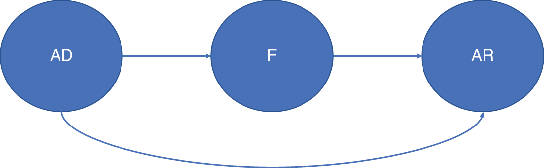
FIGURE 6.3 A third potential modeling sequence (Model C).
It is important to understand what all these alternatives mean. Assume for the sake of simplicity that we have only one variable in the alternative dataset trying to predict only one fundamental ratio, and let's focus on the case of linear regression models. In terms of equations, Model A translates into:
with the assumption that ![]() . For Model B we have:
. For Model B we have:
and for Model C:
where it is assumed that ![]() . There is no way to conclude upfront which is the best model but each modeling sequence we choose comes with assumptions with regard to the correlation (of lack thereof) between residual error terms.
. There is no way to conclude upfront which is the best model but each modeling sequence we choose comes with assumptions with regard to the correlation (of lack thereof) between residual error terms.
We must say that practical considerations will also guide the modeling choice, like the availability of data. For example, assume that we have alternative data only for a short amount of time, say, 2 years of daily observations. Company fundamentals, on the other hand, are only available at quarterly frequency or perhaps semi-annual frequency, depending on the country. This means that over the 2 years' time window, the equations used to predict ![]() (Model A and Model C) will have very low statistical power. In Model C, this also means converting
(Model A and Model C) will have very low statistical power. In Model C, this also means converting ![]() to quarterly frequency, thus losing potential variation due to lower time granularity. If the asset returns are available daily, then a better option could be to use directly Model B but with the caveat that we might sacrifice some economic intuition. We will test the three approaches in Chapter 10 on a dataset consisting of global automotive stocks, alongside an alternative dataset from IHS Markit on the automotive supply chain.
to quarterly frequency, thus losing potential variation due to lower time granularity. If the asset returns are available daily, then a better option could be to use directly Model B but with the caveat that we might sacrifice some economic intuition. We will test the three approaches in Chapter 10 on a dataset consisting of global automotive stocks, alongside an alternative dataset from IHS Markit on the automotive supply chain.
We also point readers to other literature on this subject. This includes Guida (2019), who applies machine learning for factor investing. Their study uses a machine learning technique (XGBoost) to incorporate features based on equity ratios into a factor model that trades single stocks. Alberg and Lipton (2018), meanwhile, use deep learning to forecast traditional company fundamental ratios. These forecasts are used as inputs into an equity factor trading model. We shall elaborate on this paper in Chapter 10, in our own analysis of a trading strategy on automotive stocks.
6.8. SUMMARY
In this chapter, we gave a brief introduction to factor-based investing, discussing some of the most common factor models. While factors such as trend and value are very well established and form the basis of various smart beta indices, we noted that alternative data could be used within the process to enhance existing factors and also create new ones. As we might expect, factor-based investing is usually focused on improving the return statistics for an investor. However, it is possible that investors may have other objectives, over and above purely examining returns. We cited the example of ESG datasets that could be used by factor investors to include in their investment process, considerations related to environmental, social, and governance firms. In general, firms that score highly on ESG criteria are also likely to be good investments. For example, it is unlikely that a firm that is seen as having governance issues and significant conflicts of interest would be seen as a plus by markets.
NOTES
- 1 We assume that the reader is familiar with the basics of Markowitz's portfolio theory. For those who are not, we advise the following literature: Markowitz (1991), Markowitz & Todd (2000).
- 2 See Cochrane (2009) for a derivation of the CAPM in a fundamental equilibrium approach. The “prediction” of such an approach is essentially Equation 6.1.
- 3 In theory, the market in Equation 6.1 must include all the asset classes. In practice, it is very difficult to construct such an index, so proxies are preferred.
- 4 In the case of well-diversified portfolios, one can indeed argue that the idiosyncratic errors can be neglected. However, such assumption does not always hold in practice. In fact, network effects (i.e. non-vanishing correlations) can be present among the
 and they might be non-negligible (see Billio, 2016; Ahelegbey, 2014).
 - 5 See Connor (2010).
- 6 We drop the subscripts here.
- 7 See Cochrane (2009) for the derivation of Equation 6.6 both in the absence of stochastic error terms and in their presence. In the latter case, the argument goes that diversification can remove idiosyncratic risk as error terms are uncorrelated with one another and with the factors. This, of course, might not hold because in reality, for finite portfolios, the residuals' small risk can still be priced in, or even for very large portfolios where some assets could represent large portions of the market. See again Cochrane (2009), Chapter 9, and Back (2010), Chapter 6, for a discussion on the topic.
- 8 Could be regarded as a risk premium in case of positive sign of
 .
. - 9 The book-to-market ratio is defined as the book value of a company divided by its market capitalization (a stock's price times shares outstanding). The book value is defined as the net asset value of a company (i.e. the difference between total assets and total liabilities).
- 10 Low-value stocks are also called growth stocks; high-value stocks are simply sometimes called value stocks.
- 11 Factors other than those based on accounting variables or alternative data can be of value as well. The momentum factor in the Carhart model, for example, is constructed from past stock returns, which is neither accounting nor alternative data.
- 12 Indices constructed with weights according to some risk factor (e.g. the value factor).
- 13 These are the equivalent of roughly 8.8%, 9.7%, and 11.5% compound annual returns, respectively.
- 14 https://www.indexica.com/.
- 15 In this section we will make use of the language of Probabilistic Graphical Models (PGM). For an introduction see Koller et al. (2009).