
CHAPTER 9
Outliers (Anomalies)1
9.1. INTRODUCTION
We discussed briefly in Section 3.3.4 that sometimes outliers can be an issue when dealing with (alternative) data. They can be of technical nature (e.g. a glitch) or simply a property of the data. In this latter case, we might either want to model them (e.g. fraud detection) or simply discard them as we might want to focus on modeling the “normal” portion of the data only.
The first step to treating outliers is, of course, to find them. In this chapter we will delve more into the details of how outliers can be detected. Preferably, the next step is to explain them, if required by the business application. A potential2 third step is to treat them. This means we either remove them (and in this case we fall back to the missing data problem of the previous chapter) or model them. Again, this depends on the specific problem at hand.3
In this chapter we will show some techniques to outliers' detection and explanation. The techniques – like in the missing data chapter – cannot be exhaustive for all the problems encountered in practice. However, they will be a selection of what we have seen working broadly in practice in a breadth of applications. We will finish the chapter by illustrating a use case focused on detecting outliers in Fed's communications.
9.2. OUTLIERS DEFINITION, CLASSIFICATION, AND APPROACHES TO DETECTION
Outlier detection is the process of finding those observations in data that are different from most of the other observations. Hawkins's definition of an outlier (Hawkins, 1980) states that the points must be different enough from the rest of the observations to suggest that they were produced by a different mechanism or model. There is an intuition behind this definition. While normal observations are generated by some process, abnormal points deviate from this pattern and were likely generated by a different data generating process. In these situations, they are considered to be noise, measurements errors, deviations, or exceptions. There is no single definition. In different settings the underlying meaning of an exceptional object could, of course, be different.
There are numerous situations in which anomaly detection is important: in medical data analysis, industrial production monitoring, bank fraud and network intrusion prevention, financial markets activities regulation, public health, ecosystems disturbance, and so on. One particular case relevant to trading is trying to identify anomalies within high-frequency tick data, so-called “fat-finger” data points. In Chapter 19, we discuss using high-frequency tick data from FX markets to understand market liquidity.
Recent interest in anomaly detection is mostly driven by the particular case where outliers themselves are the main problem (Tan, Steinbach, & Kumar, 2006). In fact, anomalies were historically viewed as those observations that should be found and removed from the dataset being studied in order not to disturb the patterns of normal data. Even a few outliers can distort statistical properties (such as means and standard deviations) of a set of values or the outcome of a clustering algorithm that is aimed at grouping similar observations. Therefore, anomaly detection and removal are part of data processing and, when computationally feasible, it is combined with using statistics robust to outliers.
In the context of regularity-based tasks where the normal instances are of interest, outliers are considered to be noise that should be eliminated since it can worsen the predictive or descriptive capabilities of algorithms. However, “one man's noise is another man's signal.”4 Hence, there are applications in which outliers themselves represent useful knowledge of interest, and not something to be removed. These types of outliers are frequently dealt with in telecom or credit card fraud prevention, in intrusion detection, in medical analysis, in marketing and customer segmentation, in surveillance systems, in data cleaning, in biological data analysis, and in many other fields. Within financial markets, we also need to be careful to make a distinction between fat-finger data points, which we can think of as outlying points that are likely to be reversed, and price moves that result in exceptionally volatile outcomes for other perfectly valid reasons, rather than invalid data entry.
One example of such exceptionally volatile price moves that were not the result of fat-finger errors were those of EUR/CHF on January 15, 2015. On that day, the Swiss National Bank (SNB) stopped intervening in the market to maintain a floor in the price of EUR/CHF at 1.20. The SNB had previously been trying to prevent appreciation in CHF, which would have negatively impacted Swiss exporters. However, they removed the floor following the ECB's move to begin quantitative easing. On the day the SNB removed the floor, EUR/CHF traded as low as 0.85, in the subsequent incredibly volatile price action. EUR/CHF settled in the area of 1.00 by the close of the day. It took over three years till it traded back above 1.20, hardly the sort of quick reversion we would associate with a fat-finger print.
If we think specifically about alternative data (and the structured datasets derived), it isn't always the case that outliers have a temporal structure, as we might expect in the time series for market data. There are many potential examples of outliers in alternative datasets. We may have outliers in sentiment scores based on news text, which might be unusual for a particular set of features like topic, type of article, or text length. We might either choose to remove this article, or indeed in other circumstances to flag it specifically to the user, as the unusual news could be of particular market relevance. In Section 9.8, we have a specific case study on flagging outliers in a text-based dataset for FOMC communications.
When structuring satellite imagery, we might infer various features such as the car counts, which seem anomalous compared to other similar days and locations, which could be related to many factors such as cloud cover, holidays, and so on. Later, we shall discuss the concept of local outliers, which can be “contextual.”
9.3. TEMPORAL STRUCTURE
Intrusion detection analyzes a data stream and is primarily focused on finding behavioral patterns in the data. When the pattern unexpectedly changes, an anomaly should be detected in nearly real-time, because the longer the lag, the higher the damage. In this sense, anomaly detection has a temporal connotation. A similar situation arises with fault detection systems in production line settings and in credit card fraud detection. In the latter case, the spending pattern of the cardholder is continuously checked against the attempted activity so that in case a transaction is suspicious, an alarm is raised as soon as possible.
In many fraud detection settings, historical data logs are analyzed in order to label cases that could be associated with fraudulent accounting, suspicious internet payments, or misused credit cards. Also, there are specialized situations when a post-incident or predictive analysis is conducted in order to provide early warnings of undesirable situations in the future. These specialized problems can have very efficient solutions. In a vast number of real-world situations, though, there is no distinct time structure in the data, so other methods for anomaly detection must be used.
9.4. GLOBAL VERSUS LOCAL OUTLIERS, POINT ANOMALIES, AND MICRO-CLUSTERS
An observation in a dataset can be considered anomalous with respect to just one of its attributes or a combination of several features. Since in most cases an object has multiple attributes, it can be anomalous with respect to one of them, but can be normal with respect to others.
An outlier can be classified as global when that observation is different from the whole dataset (also known as the population) with respect to a particular attribute. It can be an unusually high, low, or just a rare value. However, an observation can have a common value for each of its attributes, but still be an outlier. For example, a high salary can be quite normal with respect to the whole population, but when restricted to 18-year-olds it is an outstanding observation. When the point is different from its neighborhood while its value is not exceptional for the whole dataset, it is classified as a local outlier. In the book on data mining by Han, Kamber, and Pei (2011), a local outlier is also called “contextual,” such as our unusual news article example discussed earlier.
When using an approach of grouping similar observations (in a clustering setting) a separate category of micro-clusters can be introduced. These small groups of observations may consist of outliers, but also may consist of normal objects. Another name for a small group of outliers is “collective outliers.” In order to deal with collective anomalies, correlation, aggregation, and grouping are often used to generate a new dataset with a different representation – a “data view” (Goldstein and Uchida, 2016). In the resulting dataset, micro-clusters are represented by single points and the problem is again formulated as point outliers' detection. This chapter focuses on single-point anomaly detection, assuming that there are no groups of anomalous observations or they are small enough to recognize each point as an outlier.
9.5. OUTLIER DETECTION PROBLEM SETUP
As we discussed in Section 3.3.4, anomaly detection problem setup is traditionally divided into supervised, semi-supervised, and unsupervised. In the supervised setting, labeled data is available for training and testing outlier detection algorithms. Usually, in these cases the data is highly unbalanced (the number of normal observations far exceeds the number of outliers) because anomalies are rare by definition. Therefore, not all traditional classification methods work equally well.
Nevertheless, some of them work well with unbalanced datasets. These methods include Random Forests, Support Vector Machines (SVMs), Neural Networks, and many other methods combined with tools that address the unbalanced structure of datasets (for instance, special sampling techniques). These approaches are extensively covered in the book on statistical learning by James et al. (2013) and in the book on data mining by Witten et al. (2011).
However, in most cases, a fully labeled dataset is not available because anomalies are not known in advance. If there exists a sufficiently large dataset of normal instances (without outliers), then the problem is called semi-supervised. It is also called a one-class classification problem. Commonly used methods in this setting are One-Class SVMs (Schölkopf et al., 2001), auto-encoders, and a wide range of statistical methods where algorithms learn the normal class distribution. Hence, any new observation is assessed with respect to the probability to observe its value for the normal class. For example, Kernel Density Estimation (Rosenblatt, 1956) or Gaussian Finite Mixture Models can be employed in this case.
In an unsupervised learning setup, there is no data that is labeled normal or anomalous. It means that the outlierness scores or probabilities assigned to observations depend solely on the pattern of the data distribution in this same dataset. By the nature of unsupervised learning, there are a variety of ways to define outlying objects and methods of dealing with them.
In what follows we will look at the case of unsupervised anomaly detection. This contrasts to a more mainstream classification task. Approaches for outlier detection can be roughly classified into model-based techniques, distance-based, density-based, and methods based on different heuristics. For a detailed description of these approaches, please refer to Appendix 9.10.
9.6. COMPARATIVE EVALUATION OF OUTLIER DETECTION ALGORITHMS
Numerous algorithms can be used for anomaly detection. In order to make the knowledge practical, it is important to compare their performance, at least on a few publicly available real-life datasets from different fields of studies. These datasets (for example, from the UCI Machine Learning Repository5) provide typical data for the unsupervised machine learning setup while they are the rare cases when true labels for outliers are also available.
Goldstein and Uchida (2016) implemented the most popular anomaly detection algorithms and compared them. Table 9.1 shows real-life datasets that authors used in their study.6
The datasets were designed or preprocessed to address only point outlier detection, so the anomalies are rare, not collective, and different from normal observations. This data selection covered a range of applications for unsupervised machine learning and had different properties such as size, number of outliers, and attributes. The authors implemented the most popular algorithms with different approaches toward outlier detection. Some of them are:
TABLE 9.1 Datasets used in comparative analysis of outlier detection algorithms.
Source: Goldstein and Uchida (2016).
| Dataset | Observations | Outliers | Attributes | Comments |
| b-cancer | 367 | 10 | 30 | Breast Cancer Wisconsin (Diagnostic): features extracted from medical images; the task is to separate cancer from healthy patients. |
| pen-global | 809 | 90 | 16 | Pen-Based Recognition of Handwritten Text (global): handwritten digits of 45 different writers, in the “global” task only the digit 8 is kept as the normal class and digits from all of the other classes as anomalies. |
| letter | 1,600 | 100 | 32 | Letter Recognition: the UCI letter dataset contains features from the 26 letters of the English alphabet, where three letters form the normal class and anomalies are sampled from the rest. |
| speech | 3,686 | 61 | 400 | Speech Accent Data: contains data (i-vector of the speech segment) from recorded English language, where the normal class comes from persons having an American accent and outliers come from seven other speakers. |
| satellite | 5,100 | 75 | 36 | Landsat Satellite: comprises features extracted from satellite observations of soil from different categories, where anomalies are images of “cotton crop” and “soil with vegetation stubble.” |
| pen-local | 6,724 | 10 | 16 | Pen-Based Handwritten Text (local): here all digits are the normal class, except for the anomalous digit 4. |
| annthyroid | 6,916 | 250 | 21 | Thyroid Disease: medical data, preprocessed to train neural networks, known as the “annthyroid” dataset, where normal instances are healthy non-hypothyroid patients. |
| shuttle | 46,464 | 878 | 9 | Statlog Shuttle: the shuttle dataset describes radiator positions in a NASA space shuttle with the normal “radiator flow” class and different abnormal situations. |
| aloi | 50,000 | 1,508 | 27 | Object Images: the aloi dataset represents images of small objects taken under different conditions and broken into feature vectors using HSB color histograms. |
| kdd99 | 620,098 | 1,052 | 38 | KDD-Cup99: contains simulated normal and attack traffic, designed to test intrusion detection systems, where attacks constitute anomalies. |
- KNN is an algorithm for global outlier detection (Ramaswamy et al., 2000). It takes the distance to k-th nearest neighbor of the observation in the features space and based on this measure assigns scores of outlierness to every point in the dataset. Usually, k is in the range from 10 to 50, and a threshold for outlierness is set individually for a given dataset. Please also refer to Chapter 4 for a broader discussion of KNN.
- LOF, local outlier factor, searches for local outliers (Breunig et al., 2000). In order to get a local outlierness score, the k nearest neighbors are found for each observation. Then the local density in the neighborhood of the observation is estimated. The last step is to compare this local density with the ones for the nearest neighbors of the point. The resulting score is an average ratio of local densities. If it is around 1, the point is considered normal; if it is high, it is an anomaly. An example of LOF score visualization is shown in Figure 9.1.

FIGURE 9.1 An example of LOF score visualization in 2 dimensions: radius of a circle around each point represents its score.
Source: Wikipedia, https://commons.wikimedia.org/wiki/File:LOF.svg. Public Domain. Retrieved: 6 August 2018.
- CBLOF is a cluster-based outlier factor algorithm (Goldstein, 2014). Clustering (usually, k-means) determines areas in the attributes space where observations are grouped. The outlierness score is calculated based on the distance of an observation toward the nearest cluster center. It depends on parameter k and gives different results for different runs due to the randomness of k-means.
- HBOS is a histogram-based statistical outlier detector (Goldstein and Dengel, 2012). For each attribute a histogram of values is built and for an observation its score is equal to the inversed product of histogram heights across all histograms. This method ignores dependence between attributes, but it is fast and works particularly well in high-dimensional sparse datasets. Parameters in HBOS determine the way bins are formed, which can affect outcomes.
- One-Class SVM (Schölkopf et al., 2001) estimates the area in the attributes space where normal observations are concentrated. This method is usually used in semi-supervised setup, but it is also applicable to unsupervised problems as by assumption outliers are rare and the soft margin optimization procedure allows the model to be trained to have only a few outliers. The outlierness score is based on the distance of an observation to the boundary of the area of normal cases. Please see Chapter 4 for a more general discussion of SVM.
An industry standard for comparison of unsupervised machine learning techniques is to rank all observations by scoring outputs and then iteratively apply a threshold from the first to the last rank. This results in a collection of pairs of true positive and false positive rates, which forms an ROC curve. The area under this curve is denoted AUC and represents the performance measure. The AUC can be interpreted as the probability that an algorithm assigns a randomly chosen normal instance a lower score than a randomly chosen anomalous instance (Fawcett, 2006).
Findings in Goldstein and Uchida (2016) show that local anomaly detection algorithms, such as LOF, perform poorly on datasets containing only global anomalies because they generate many false positives (they label normal observations as outliers). At the same time, global anomaly detection algorithms perform average or better than average on problems where only local outliers are present. Therefore, if the context of the data is not known a priori, it is better to choose a global anomaly detection algorithm.
Goldstein and Uchida (2016) infer that in most cases KNN-type algorithms perform better and are more stable than clustering approaches. On the other hand, clustering algorithms have lower computation time, which is crucial for large datasets or in near real-time setting, but can be detrimental for small datasets. It is shown that a variation of CBLOF performs well on average and can be used as a cluster-based method where appropriate. The final recommendation is to implement KNN, LOF, and HBOS, which shows good results in the comparative evaluation and works fast, especially for large datasets. We should be careful to note that some of these techniques might be amenable only to non-temporal numeric datasets.
9.7. APPROACHES TO OUTLIER EXPLANATION
There are numerous approaches to anomaly detection in an unsupervised setup with hundreds of algorithms implemented. But even when an expert from a particular field of study gets output from these methods, it may be unclear exactly why these observations have been chosen as outliers.
Some of the methods provide intuitive explanations as a byproduct of the anomaly detection process, but those explanations are applicable only to the observations picked by the methods. For example, a decision tree would give a set of rules as an output, stating that when some of the attributes exhibit values above or below particular thresholds, then an observation is classified as an outlier. Otherwise, it is classified as a normal instance. Such a method cannot explain outlierness of an observation if it does not consider this observation to be an outlier.
On the contrary, the outlier explanation task is aimed at describing what distinguishes an observation from the rest of the dataset. If attributes of the dataset are meaningful to the subject expert, then an explanation can help him or her to understand the underlying reason for outlierness, regardless of whether an algorithm has labeled that instance as an anomaly. It implies that an explanation should be intuitive and concise. A classical approach to explanation is to plot the dataset, where a point outlier or an outlying micro-cluster can be seen. But visualization requires an attribute subspace, where other objects are distributed around the labeled outlier in the way that demonstrates its anomalousness. Moreover, multiple subspaces might be provided to aid explanation.
Recently, a number of studies suggested other approaches to outlier explanation, where some methods return a combination of attributes that distinguishes an outlier while others derive different kinds of association rules (like in Agarwal et al., 1993). An explanation could be a byproduct of outlier detection as well as a separate problem. In what follows we summarize the works of Micenkova et al. (2013), Duan et al. (2015), and Angiulli et al. (2009, 2017). These solutions were chosen based on their comprehensiveness, applicability in different situations, ease of implementation, and computational complexity.
Similar to the outlier detection task, it is important to compare and evaluate explanation algorithms. Considerations in the article by Vinh et al. (2016) laid the base of the analysis. After a primary approach is selected, it is always possible to leave an opportunity to switch to another one in case the results do not meet expectations.
9.7.1. Micenkova et al.
The method of Micenkova et al. (2013) suggests separating an outlier from the normal instances in its neighborhood by a linear boundary and then turning the problem of separation into a classification task. Under the assumptions of the method, features that have the highest importance in classification are those that demonstrate the outlierness of the observation. This method is claimed to work well, but appears to be “local.” According to Angiulli (2009), its locality makes a difference in case there is a small cluster of observations that are different from the vast majority of others that do not fall into the small neighborhood of an outlier in focus. Also, in some cases outliers and the normal neighborhood cannot be separated by a linear boundary (see Figure 9.2).
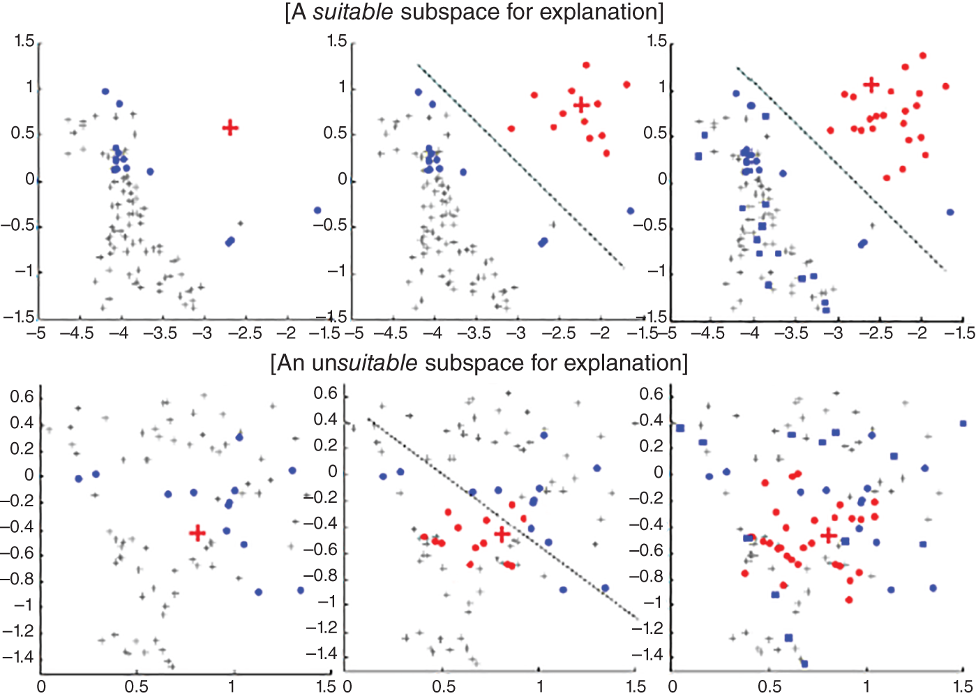
FIGURE 9.2 An illustration of potential difficulties in choosing a normal neighborhood (subspace) around an outlier in order to separate them with a linear boundary. Normal instances chosen to represent the neighborhood are highlighted with dark while lighter circular points around the outlier-cross represent a synthetic normal distribution generated to be an outlier class in the classification task.
Source: Adapted from Micenkova et al. (2013).
Making a comparative evaluation of different approaches to the problem of outlier explanation, Vinh et al. (2016) notes that, while the feature selection–based approach works well, there are two important points. First, the k-nearest neighbors in the full attribute space may be significantly different, or even totally different, from the k-nearest neighbors in a subspace. It means that the neighbors in the full space are not necessarily representative of the locality around the outlier in subspaces. Therefore, an object can be well separated from its k-nearest full-space neighbors while in fact not being well separated from its subspace neighborhood.
The second potential drawback of this approach based on feature selection is concerned with the spread of the synthetic distribution that represents an outlier in the classification task. It depends on the k-nearest neighbors distance in the full features space and does not take into account differences among subspaces. Although some subspace can be a good explanation (the point being a local outlier), the feature selection approach may eventually rule out this subspace as the synthetic distribution heavily overlaps with the normal neighborhood.
9.7.2. Duan et al.
A different paradigm for outlier explanation is suggested in the work by Duan, Tang, and Pei (2015). The problem of explaining outlierness is defined as a search for a subset of the attributes space where the observation is outlying the most. In order to measure outlierness, the authors rank probability densities of all observations in a subspace of features. Roughly speaking, they rank all the observations with respect to how rare their combination of values for the chosen features are. A minimum in terms of dimensionality subspace where the anomalous object is ranked the best (the most exceptional) is returned as an explanation.
The approach of Duan et al. (2015) seems to be more comprehensive for a subject expert who conducts outlier explanation. Its drawback is in computational complexity of estimating probability density functions for all attribute subsets of the dataset. And, as mentioned in Vinh et al. (2016), rank statistics do not always choose the subset that describes outlierness of an object in the best possible way. For example, density rank may be high in a subset even though the point is not far away from the rest of the observations while in another subset the object could be an obvious outlier, but its rank can be lower (see Figure 9.3).
It is interesting to note, that in Vinh et al. (2016) a thorough exploration of outlierness measures is conducted with a focus on the fact that a proper measure should not depend on the dimensionality of the subspace where it is employed. According to the study, good candidates for the role of outlierness measure would be: the Z-score (normalized density function for an observation in a subset, as suggested in Vinh et al., 2016), isolation path length (a normalized length of a path to an outlier in an isolation tree, as suggested by Liu et al., 2012), and LOF score (as introduced by Breunig et al., 2000) formally satisfy dimensionality unbiasedness.
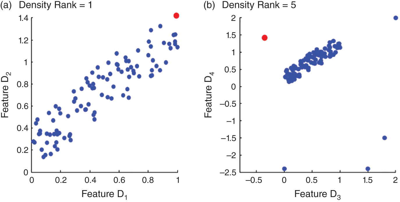
FIGURE 9.3 An illustration of a case where rank statistic does not provide the best explanation of an outlier (shown as a light shade of grey). It returns features D1 and D2 while the best explanation would be to return features D4 and D3.
Source: Adapted from Vinh et al. (2016).
It is noted that the density Z-score exhibits good performance but is computationally expensive, so it is only applicable for small numeric data sets. On the other hand, the isolation path score is an effective measure that also demonstrates good performance, making it suitable even for large datasets. Its limitation is that isolation path is not designed to detect local outliers, though it is likely that no measure is optimal in all possible settings.
The techniques (Micenkova et al., 2013 and Duan et al., 2015) are representatives of two different categories of approaches: those based on features selection and those based on score and search. Vinh et al. (2016) discuss the connection between these two approaches and propose a hybrid solution.
9.7.3. Angiulli et al.
The last of the three approaches considered in this chapter is suggested by Angiulli et al. (2009, 2017). It focuses on modeling outlierness relative to the whole dataset or a homogeneous (that is, consisting of similar observations) subset around an outlier. It is a more technical, but also the most contextual, way of explaining outliers.
For a dataset with categorical attributes and a given outlier, Angiulli et al. (2009) find the top best subsets in which the outlier receives the highest outlierness scores with respect to a single attribute. The outlierness measure is calculated as a linear combination of the frequency and an analog of a Gini index of statistical variability of the attribute values in the subset. In the later work, Angiulli et al. extend and change the framework to deal with continuous numeric features, too.
The fact that the outlierness is always calculated with respect to a single attribute while the subset of observations (neighborhood of an anomaly) is always in the full feature space makes a consistent comparison possible. It results in that the problem set-up satisfies the desired properties of outlierness measures, summarized in Vinh et al. (2016).
If the abnormality of a given outlier is established with respect to the entire dataset, it is a global outlier. Otherwise, if the value is outlying for a subset, it is a local outlier. In the first case, the explanation is that an attribute exceeds its abnormality threshold. The second case is more complicated. A data point that is not an outlier relative to the whole dataset is considered an outlier relative to a subset containing it. In this setting, if an outlier is not rare compared to the rest of the objects in the dataset, no outlying features are detected.
A dataset on skills/age in Angiulli et al. (2009) provides an example of a situation where this approach gives a meaningful explanation of outlierness while the Duan et al. (2015) and Micenkova et al. (2013) do not. In the example, skills developed by employees are measured against their age. An outlier in focus is a young 18-year-old individual who exhibits a high level of skills. Under Micenkova's approach, local separability may be misleading because the nearest neighbors of the outlier can actually be anywhere below or to the right of the observation. It means that weights of age and skill features in a separation task would be misleading. The approach by Duan would return a subset of attributes equal to the whole set because low probability density of the object is exhibited only in the joint space of skills and age.
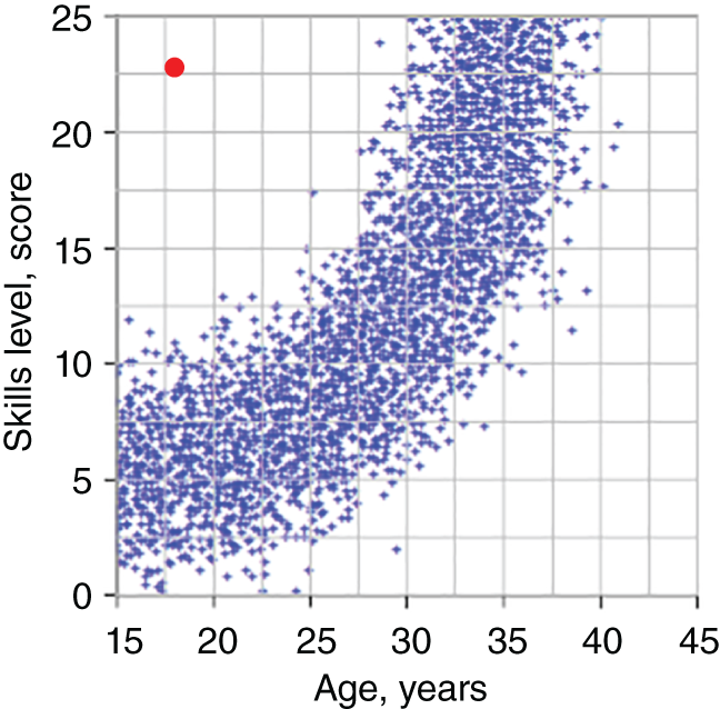
FIGURE 9.4 Outliers explanation in problematic situations: measuring skills versus age of employees. The outlier is highlighted in a light shade of grey in the top left corner.
Source: Adapted from Angiulli et al. (2009).
At the same time, if the explanatory subset under the Angiulli framework is the subset of people who are 18 years old, and the outlying attribute is the skills level, then the considered individual becomes a clear outlier, as demonstrated in Figure 9.4.
Besides other technical details, there are some substantial differences between the approaches suggested by Micenkova, Duan, and Vinh, and the approach devised by Angiulli (2009, 2017). Angiulli assumes that outlierness is relative to the whole dataset in the full attributes space. Other methods return individual subspaces where the query object is outlying the most compared to the other subspaces.
Keeping this in mind, it becomes clear that the approach suggested by Angiulli et al. (2009, 2017) can turn out to be the most applicable. First, it is developed both for categorical and numerical data, even though the approaches are not exactly the same. Second, it measures outlierness only with respect to a certain attribute, so calculations are always univariate (involving a single variable). The only point where subsets matter is when a subset of the whole dataset is taken as a neighborhood of an outlier. And last but not the least is that the explanation provided is the most contextual among peers.
The “contextual” approach to explanations mining is covered in two articles by Angiulli et al. In the 2009 work the authors focus on the case of categorical attributes, introduce an outlierness measure, build a general framework for further explanations mining, and develop a tree-based search to get the top pairs of explanatory subsets and outlying attributes. In the 2017 work the authors concentrate on tackling continuous numerical data, introducing probability density function estimation for an outlying attribute, amending the outlierness measure so that it is applicable to probability density functions rather than frequencies, and introducing a novel method to prune subsets when building explanations for outliers.
9.8. CASE STUDY: OUTLIER DETECTION ON FED COMMUNICATIONS INDEX
In this section, we show a practical use case of using outlier detection on an alternative dataset related to financial markets. We use as our dataset a preliminary version of Cuemacro's Fed communications index. The raw data consists of various Fed communications events. These events are speeches from the Fed's Board of Governors and Regional Fed presidents, FOMC statements, FOMC minutes, and various other types of Fed communications. These Fed communications to the market are collectively referred to as Fedspeak. The Fed regularly provides information to the market through these methods in an effort to be more transparent in how they operate. This approach is also consistent with the way many other central banks also interact with the market.
For each Fed communication event, we have a number of other fields, which have been tagged. These include:
- Date of the Fed communication
- Event type of Fed communication (e.g. a speech, an FOMC statement, etc.)
- Speaker (e.g. Chairman Powell)
- Audience (or location) of the communication
- Text of the communication
- Title of the text
- Length of the text
- CScore of the text
A proprietary algorithm is run on the text of each communication to create a CScore for that text, which is indicative of the underlying sentiment of that text. These CScore values are then aggregated across all the various Fed communication events, to create an index representative of overall Fed sentiment based on Fed communications. In Chapter 15, we discuss the index in more detail, showing how it can be used to understand the moves in UST 10Y yields.
While the text data is publicly available on the web, there are various challenges when collecting it. In particular, the sources are from a diverse array of websites. It requires a lot of maintenance to do such web parsing on an ongoing basis. It involves both updating code and performing manual checks. While this is a time-consuming and labor-intensive process, the problem of maintenance is tractable.
Another potential problem is that when backfilling the history of Fed communication events, we need to read a large number of archived websites. Their formatting can be substantially different, and often does not have a consistent format with the newer pages on the same websites. Hence, we face having to deal with myriad different webpage formats, even if they appear to be from the same website. This might result in problems in web parsing some of the history, and additional time spent to check anything we parse, as well as more time writing code.
The volume of historical texts in our dataset of Fed communication events is around 4000, and covers approximately 25 years of Fedspeak. While the history is quite comprehensive, w note that it does not include absolutely every Fed communications event during this period. From the outset, we have excluded a number of texts from any further analysis. This includes any text for which we do not have any license and access to such as those behind paywalls. We also excluded video interviews from Fed speakers. In fact, in order to extract text from video interviews, we would need to have access to the video data (and appropriate licenses).7 Regardless, often text on a webpage relating to video interviews comes with a text summary. However, it is only a short summary, which may be insufficient to gauge sufficient meaning.
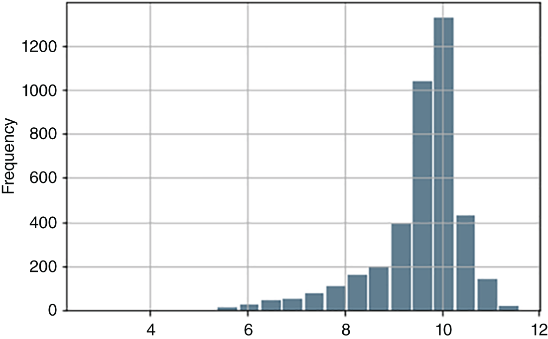
FIGURE 9.5 Histogram plot of log(text length).
Source: Federal Reserve, Cuemacro.
After this initial process of excluding various Fed communication events, we need to be able to historically identify outliers in the dataset in a relatively automated way. Any outliers that are flagged in this way would need further manual investigation, to assess whether these Fed communication events should be included in our final dataset. We have the problem of wanting to include relevant Fed communications events in our index while excluding those that are spurious.
Our first attempt at outlier detection involved creating features for what we thought identified “unusual” Fed communication events. We shall explain how we created these now. First, we created variables for measuring log(text length). Figure 9.5 shows a histogram plot for the log(text length). We have used the logarithm as the variation of text lengths of the various Fed communication events is substantial. From Figure 9.5, we could define unusually short texts as those with log(text length) being those less than 6.
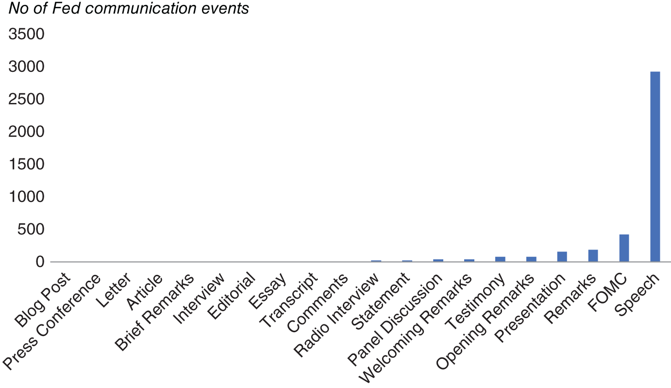
FIGURE 9.6 Event types of Fed communication.
Source: Federal Reserve, Cuemacro.
We also counted the event types of these Fed communications, which we report in Figure 9.6. This could help us assess whether there were any event types that were particularly “unusual.” In around 4000 Fed communication events around 75% are speeches by Fed speakers. The next most common Fed communication events were FOMC statements/minutes/press conferences, at around 12%. The rest were made up of events such as panels, essays, and the like, which are more “unusual.”
In Figure 9.7, we have plotted the histogram of CScores, which as we noted earlier represent the sentiment of the text associated with each Fed communication event. We can see that the vast majority of the scores are roughly in the range of −2/+2. Hence, a simple way to identify unusual CScores is just to flag anything outside that range.
We also counted the number of Fed communication events that were associated with specific Fed speakers. Figure 9.8 reports the 20 most “talkative” Fed speakers during our 25-year history of Fedspeak. Top of the list is the FOMC, which encompasses Fed communication events such as the release of FOMC statements and also FOMC minutes. Following that, we see that President Bullard has the largest number of Fed communication events. Among market participants, Bullard is known for communicating to the market quite often, so this perhaps is not surprising. Note that Yellen appears twice, once for her tenure as Fed chair and also for her tenure as president of the San Francisco Fed prior to that.
By contrast, there are some speakers historically who only appear a handful times in our Fed combinations dataset such as Gov. Lindsey. There can be a number of reasons. One can be the duration of their tenures. A fairer way to show this data, to adjust for this, could be to annualize the figure, calculating the number of Fed communications events per year for each speaker, than for their entire tenure. However, despite this, even if we adjusted this data, there can be a wide variation in how often Fed speakers communicate to the market.
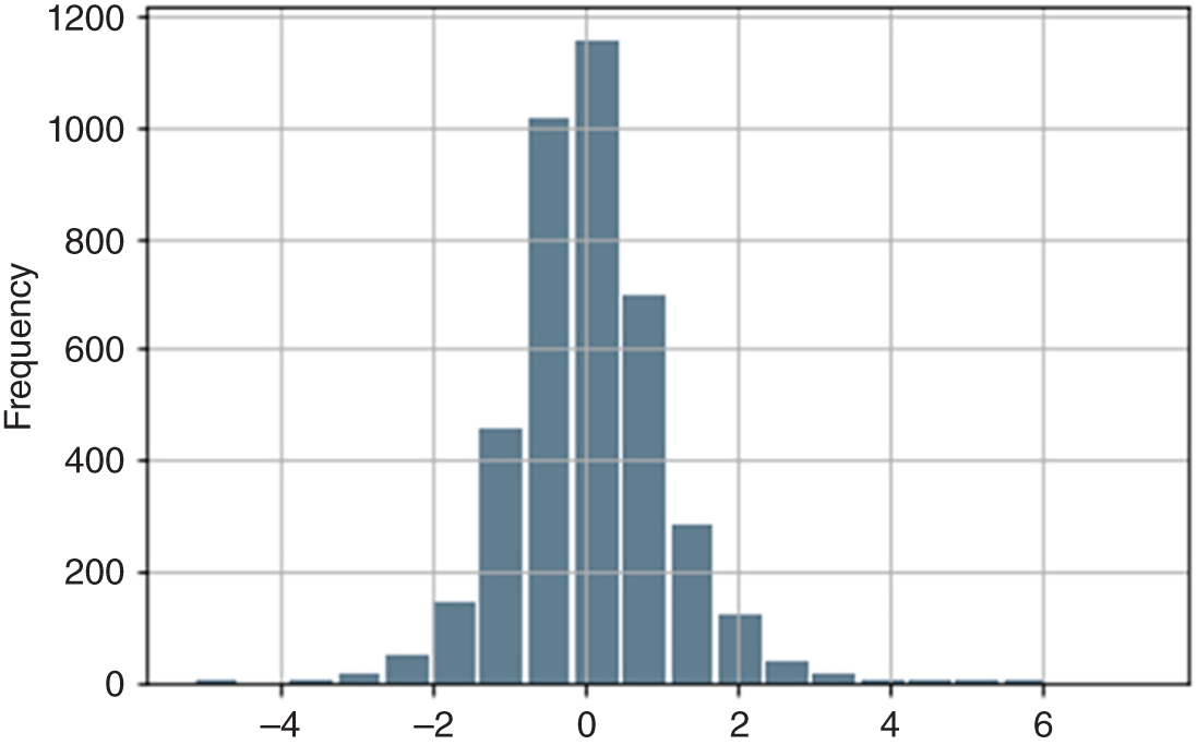
FIGURE 9.7 Histogram plot of CScores.
Source: Federal Reserve, Cuemacro.
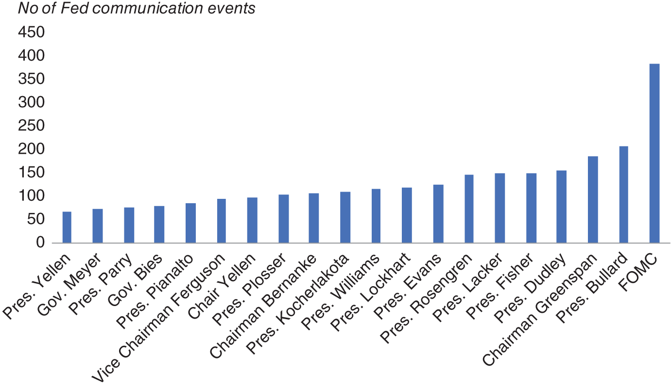
FIGURE 9.8 Most talkative Fed speakers.
Source: Federal Reserve, Cuemacro.
Another complicating matter is that in practice, the market impact of Fed speakers is not always consistent. This can make it trickier to define if a Fed communications event is an outlier by examining the speaker. For example, we might expect that those Fed speakers who are voting members of the FOMC would have more impact on the market from what they say. Voting members of the FOMC have a more active role in changing Fed policy. The FOMC has 12 members. There are 7 permanent members from the Federal Reserve Board of Governors, which includes the Fed chair. The president of the New York Fed is also a permanent member. There are then 4 rotating members of the FOMC, drawn from the presidents of the regional Fed banks. These rotating members serve for 1 year. It should be noted that regional Fed bank presidents still take part in the meetings of the FOMC and take part in discussions around Fed policy and the Fed's assessment of economic conditions. We would also expect more focus from market participants on communications given by the Fed chair.
To summarize the above points, our rules-based approaches for identifying if Fed communications were “unusual” were based on the following:
- Unusual Fed speakers (such as Governor Lindsey who only appeared a handful of times in history as speaker)
- Unusual event type of Fed communication (such as “Editorial,” which only appears very rarely in the history)
- Unusual CScores – i.e. extreme values (outside of −2/+2)
- Unusual log(text length) – i.e. very short texts (less than 6)
Hence, based on these various heuristic measures we have used, outliers are likely to consist of those Fed communication events that have characteristics such as shorter texts, extreme CScores, unusual event types, and are also from a speaker who communicates comparatively rarely to the market. It can be trickier, though, to precisely articulate the relative impact of each variable when combining these flags. Note that we avoided using some variables such as the audience/location of Fed communication events when flagging for an outlier. In this instance, it is difficult to think of an intuitive reason why the geographical location of a Fed speaker's speech would necessarily make it an “outlier” from the perspective of how the market interprets the communication. Furthermore, there are a very large number of locations and audiences that are not repeated in the dataset and are unique, making it difficult to come up with specific rules for flagging which are outliers.
Obviously, in all these cases where we are creating outlier flags, we are attempting to use our own domain knowledge of Fed communications in order to create indicators by hand to help identify unusual Fed communication events to be labeled as outliers. However, in practice, we might wish to have a more automated way of identifying outliers, particularly when backfilling the history, when the volume of communications is too high to check manually. Such automated methods can also take into account a combination of different variables tagged for each Fed communication event. We earlier noted that it might be difficult for us to formulate precisely how combinations of input variables are indicative of outliers.
In order to do a more automated approach, we used unsupervised ML techniques for detecting outliers, namely:
- k-means
- HBOS (histogram-based outlier score)
- HDBSCAN (hierarchical density-based spatial clustering of applications with noise)
- KNN (k-nearest neighbors)
- ISO (isolation forest)
In each instance, the algorithms were set to identify the most unusual 1% of cases, which corresponded to around 40 Fed communication events from our dataset of around 4000. These methods search for points that appear to be outliers away from the main cluster of points. We should note that in a production environment, such outlier analysis would need to be done on a rolling basis, rather than looking at the entire history. In order to use these techniques, as with our rules-based approach earlier, we needed to select input variables for each Fed communication event. Unlike in our rules-based approach, we did not specifically create cutoff points to define when each of these input variables constituted an outlier. For those variables that were categorical, there are several ways to encode them. If the number of unique categories is below a threshold, they are one-hot-encoded. Essentially, the categorical variable is replaced by several binary variables. For example, if we are encoding speakers this way, we'd have a binary variable to represent if Chair Yellen is the speaker (or isn't), another one for Chairman Bernanke, and so on. In other instances, the categorical variables are reduced to an analog of “value-of-information,” which is a single column with values based on frequencies of a corresponding category.
We used the following input variables, which were a mix of both categorical and continuous variables:
- The speaker – categorical variable
- The event type of Fed communication – categorical variable
- Log(text length) – continuous variable
- CScore of the associated text – continuous variable
In general, most of the outliers flagged by these various unsupervised ML techniques or when flagging by extreme CScores tended to be associated with shorter texts. This seems intuitive, as it can be more difficult to ascertain the sentiment of the text when we have less text to parse. These events included presentations that typically have only a short summary of text associated with them. In some cases, Fed communication events were flagged as outliers because the texts were incomplete due to problems in parsing. Other reasons included mislabeling of various tags such as spelling mistakes on the speaker's name or an incorrect event type (which include slightly different labels for what are essentially similar events). In these instances, the “outlier” issue can be solved by parsing the text again, by modifying the approach to web parsing and also changing the tags. Once this is done, the newly read text would also need to be manually checked. Any new tags would also need to be checked. Such Fed communication events could be updated in the history, with the cleaned fields.
Roughly half of outliers were explained by variables associated with the text themselves (such as the length or the CScore) and/or combinations. For example, it might be that the CScore was unusual for the text that was provided. Most of the remaining strong explanations were related to speeches being unusually long texts or a rare CScore for such a long text.
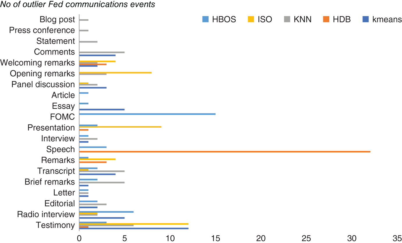
FIGURE 9.9 Event types of Fed communications flagged as outliers by unsupervised ML techniques.
In terms of the unsupervised techniques, k-means tended to work best for flagging outliers, which seems understandable given the relatively wide spectrum of Fed communication events that are present in our dataset.
In Figure 9.9, we tally the total number of event types of those Fed communications events that were flagged as outliers by the various unsupervised models we discussed earlier. We note that k-means tended to flag unusual event types of Fed communications such as testimonies, which did not appear often in the dataset. Many of those events flagged as outliers would likely be considered as unusual or as special events by a domain expert such as an economist who reads Fed communications on a regular basis. Typically, testimonies are widely followed by the market, in particular when given by the Fed chair, as they can give a wide-ranging insight into Fed policy, given their length and also because of the many questions they face from lawmakers during such testimonies. One particular, noteworthy example of a Fed testimony which moved markets was Chairman Bernanke's testimony to Congress where he hinted at the winding down of quantitative easing. The resulting “taper tantrum” saw bond yields rising significantly.
This contrasts to HDB, which seemed to flag mostly event types such as speeches, which as noted earlier appear very regularly in the Fed dataset. This is also true of HBOS, which appeared to flag quite a few FOMC events that are again quite common in the dataset. While it is difficult to make any generalization about other datasets, in practice many of these Fed communication events, which were judged to be outliers by HDB and HBOS, would be less likely to be flagged as outliers by domain experts. Indeed, it would be extremely unusual to remove FOMC events such as statements and minutes, given that these are events where Fed policy changes are announced and explained to the market.
We should also note in closing that we could try combining both approaches, such as flagging outliers that satisfied our rules-based approach (such as those we have flagged as short texts), while also picking texts that were deemed to be outliers by an unsupervised approach such as k-means.
9.9. SUMMARY
We have examined a series of techniques for outlier detection and explanation. Again, the no-free-lunch theorem applies here as well – there is no universally best-performing algorithm but everything depends on the context and the specific problem at hand. Sometimes outliers are the result of technical glitches and/or recording mistakes – something that we said is occuring a lot in the alternative data world. In this case, they can be eliminated and will be again in the missing data domain. Sometimes, they are properties of the data-generating process and need to be explained and modeled separately. Hence, having the right toolkit of techniques is essential in the alternative data world. We glimpsed some of them but we are aware that there are many more with each application calling for its own best method.
We examined a real-world case study focused on a dataset of Fed communication events such as speeches, FOMC statements, and minutes. Each event had associated fields such as the text of the communication, the date of the communication, and the like. We approached the problem of finding outlying Fed communication events in two ways. First, we tried a simple rules-based approach. We created our own indicators to flag outliers based on extreme values of variables such as sentiment score of text, the length of each text, and so on. We then defined extreme values of these based on fairly simple approaches such as looking at the tails of histograms when plotting these variables.
Second, we used unsupervised ML techniques for detecting outliers on the dataset, rather than specify specific rules. This approach could more easily pick out outliers based on combinations of variables. Furthermore, we did not necessarily need to define what we thought was an extreme value for each input variable. Instead, we defined the proportion of values that we wanted the algorithm to define as outliers. We found that k-means was best to pick out more unusual Fed communication event types, such as testimonies, which do not appear that commonly. This contrasts to other methods, such as HDB and HBOS, which seemed to pick out speeches and FOMC events respectively. Typically, FOMC events such as statements and minutes are the most widely followed Fed communication events. Many domain experts would agree that these are very important for understanding Fed policy, and generally these should not be classified as outliers to remove from such a dataset.
9.10. APPENDIX
Approaches to do outlier detection can be roughly classified into model-based techniques, distance-based, density-based, and methods based on different heuristics. We describe them in detail in what follows.
9.10.1. Model-Based Techniques
In a semi-supervised or supervised setup, a model of the data can be built. Under supervised learning the data labeled as normal/anomalous is used to train the model to recognize outliers. In a semi-supervised setting, data that does not fit the model of normal data is the target.
For example, a statistical approach would generally estimate the data distribution and any object whose value has low probability within the framework is considered an anomaly. Most of the classical methods assume Gaussian or mixture of Gaussian distributions for the normal data and use tests based on the properties of this distribution, like Grubb's Test for Outliers, Dixon's Q Test, Chauvenet's Criterion, or Pierce's Criterion. Barnett and Lewis (1978) listed about a hundred discordancy tests for different distributions, with known/unknown parameters, different numbers of expected outliers, and their types.
In some cases, it is difficult to build a model because the underlying distribution of the data is hard to estimate or when no training data is available. In this case other approaches must be employed.
Many modern approaches to outlier detection involve statistical methods. They estimate the probability of observing an attribute value compared to any other value for the dataset in focus. Also, they often rely on association rules mining (as in Agrawal, 1993) where the key measures are support – how often a combination of values is observed, and a measure of dependence – how often two values occur together. This type of analysis is called rules-based, as opposed to classical model-based approaches.
9.10.2. Distance-Based Techniques
If a distance measure can be defined in the multidimensional space of attributes, then anomaly detection can be implemented by finding objects that are distant from their neighborhoods or from centers of nearest clusters. In cases where data can be visualized in 2D, outliers are the points that are best separated from other points. Separability is an alternative measure of outlierness – how easy it is to distinguish the point from its neighborhood.
Distance-based anomaly detection has been introduced by Knorr and Ng (1996) to overcome the limitations of statistical methods. An object is called a distance-based outlier with respect to parameters k and R if less than k objects in the dataset lie within distance R from it. This approach is based on density in a fixed-size neighborhood of the observation in the attributes space with Euclidean distance. This definition was later modified by different authors to relax reliance on the fixed radius. For instance, by taking the k-th neighbor distance instead of fixed radius, or taking an average distance toward k neighbors, and so on.
Distance-based approaches make no assumptions on the distribution of the data, as opposed to model-based statistical techniques. It makes them more flexible and universal. Moreover, in the case where the underlying distribution is known and a statistical approach is used, distance-based anomaly detection methods are a generalization of the definition of outliers in statistics, so that the larger the distance measure toward an observation, the less likely it comes from normal observations distribution (Angiulli et. al, 2009).
Distance-based methods can work well even when there is no geometric intuition behind the distance metric used. Another valuable property of these techniques is that outlierness scores are monotonic nonincreasing with respect to the amount of the data used to calculate them. This results in effective pruning rules and highly efficient algorithms.
9.10.3. Density-Based Techniques
In cases where the attribute space has a distance measure, it is possible to estimate the density of an object's neighborhood in the dataset. Based on this density and the density of the neighborhood, it is possible to pick the observations that are rare with respect to others and hence can be considered to be anomalous. (This idea was introduced by Breunig et al., 2000, with the Local Outlier Factor measure, LOF, and discussed earlier in this chapter.) The basis for high outlierness score is low relative density around an observation.
In contrast to distance-based definitions that declare as outliers the points where data density is low, density-based approaches score points on the basis of the degree of unbalance between density around an observation and the estimated density of its surrounding points. As a result, these approaches are more focused on detecting local outliers, for example, lying on the border of a cluster. If the dataset consists of groups of observations that are clustered and have different densities, density-based techniques prove to be effective in finding anomalies in the space between clusters.
Density-based approaches can rely on any adequate dissimilarity function even in case there is no usual distance measure available. However, quite often the resulting outlierness score lacks explanatory power and calculations become restrictively complex in higher-dimensional spaces. Moreover, density- and distance-based approaches are susceptible to the “curse of dimensionality,” as with the growth of dimensionality it becomes harder to find adequate neighborhoods of an observation. Ideally, outlierness measures should not depend on data dimensionality.
9.10.4. Heuristics-Based Approaches
In high-dimensional datasets, angles between vectors (cosine distance) are more robust and convenient to use than distances (Kriegel et al., 2008). This is particularly true in case of sparse datasets, for instance, in text processing problems. Angle-Based Outlier Factor (ABOF) method scores observations by the variability of the angles between a point and all other points in a pairwise manner.
Isolation-Based Outliers, introduced by Liu et al. (2012), are defined as observations in a dataset that are prone to be isolated quickly under random successive splits of a random feature until all points are isolated in separate leaves of the resulting random tree. Since anomalies are few and different from the rest of the data, they are more susceptible to isolation. This approach is fast and works surprisingly well on real-life data. Moreover, it suggests a valuable measure of outlierness, equal to the normalized length of an isolation path. This measure is dimensionality-independent, and together with Z-score (analog of Mahalanobis distance) is a decent choice to use in subset mining problems, whether it is outlier detection or outliers explanation (suggested by Vinh, 2016).
Isolation Forests can be applied only to ordered attributes and are not designed for use with categorical data. Also, they tend to lack explanatory power. But in an ensemble of outlier detection methods they are highly recommended to provide results independent from those obtained from other methods.
Another class of anomaly detection methods relies on clustering techniques, where a small cluster can consist either of outliers or not (Kaufman & Rousseeuw, 2008). High- and low-density clusters are first identified. Then the data is divided into two non-overlapping sets of outliers and non-outliers and a ranking is assigned to each observation, reflecting its degree of outlierness.
NOTES
- 1 Special thanks to Kate Lavrinenko for her contribution to this chapter.
- 2 “Potential” because we might well want to stop at the second step.
- 3 We must note that some data vendors might want to treat the data themselves (e.g. missing data imputation, outliers' removal, etc.) before selling it onwards, as discussed previously in Section 5.4. Some more sophisticated buyers might prefer data vendors not to perform this step for them but rather to buy the raw preprocessed data directly. They fear is that by preprocessing the data, data vendors might discard precious information that can be useful for them later at the modeling stage.
- 4 This quote is commonly attributed to Edward W. Ng (1990), though its variations go back to Lucretius, around the first century BCE.
- 5 UCI Machine Learning Repository, available from: https://archive.ics.uci.edu/ml/index.php. Retrieved July 17, 2018.
- 6 Datasets used are available from: https://dataverse.harvard.edu/dataset.xhtml?persistentId=doi:10.7910/DVN/OPQMVF. Retrieved: July 17, 2018.
- 7 In case we had access, we would need to extract text from any video to create our own transcripts. Even if we were able to download the video interviews, we would subsequently need to do speech-to-text transcription of this data. This would not be difficult because there are many APIs, some of them available at almost no cost, able to do the transcription (e.g. from Google, AWS, IBM Watson).