CHAPTER 15
Text, Web, Social Media, and News
15.1. INTRODUCTION
The notion that text-based data is useful for trading financial markets is not an unusual concept. After all, news has been a major driver of trader behavior and prices for centuries. What has changed in recent years is the sheer quantity of text-based data that a trader might need to look at, in particular driven by the advent of the web. There is simply too much text for any human to read and interpret. We need to turn to machines to help us extract value from this huge quantity of text for us to use in the investment process.
In this chapter, we begin by exploring how to read web data. We then give many use cases for text from an investor viewpoint. We look at social media and show how it can be used to understand ideas such as market sentiment and to help forecast US change in nonfarm payrolls. Later, we will focus on newswire data and develop systematic trading rules by using it for FX markets. We will also discuss how to aggregate Fed communications and apply NLP to it to understand the movement in US Treasury yields. Lastly, we will talk about making estimates for CPI using web-sourced data from online retailers.
15.2. COLLECTING WEB DATA
The web was invented in 1989 by Tim Berners-Lee while he was working at CERN. Obviously today, over 30 years later, the amount of content available on the web has mushroomed. The web can encompass content such as news, social media, blogs, corporate data, and so on, but it also contains non-textual content, such as images, audio, and video. Some of it is freely available while other parts have restricted access, such as newspapers behind paywalls. Because content on the web originates from so many disparate sources, it is perhaps not surprising that it is predominantly in an unstructured form and does not fit into some standardized formats. Hence, if we wish to aggregate data from a large number of web-based sources, a significant effort is required to structure different sources. The huge amount of text available means that to get a true sense of it, we need to use automated methods not only to collect the data but also to decipher its meaning.
To collect text content from the web we can use an automated program, a web crawler (or spider) that systematically browses through web pages to start downloading the content. Obviously, there are too many websites to be able to browse the whole web, so typically we need to guide our web crawling. Even search engines (which seek to index the web with significant computational and bandwidth resources) using web crawlers are unlikely to be able to catalogue the entire web. Furthermore, content owners might choose to restrict the access of web crawlers and might have terms of usage that restrict automated processes. In Chapter 3, we discussed some of the legal points around the collection of data from the web.
Once we have found a specific web page of interest, the next step is understanding the content. Getting content from a specific web page utilizes “web scraping,”1 which typically involves:
- Downloading the content of the web page into its raw form
- Assigning a time stamp for the time the web page was scraped (and also, if possible, another time stamp for when the content was created)
- Removing HTML tags
- Identifying metadata such as the page title, hyperlinks, and so on
- Capturing the body text of page
- Getting multimedia content (such as images)
We can then store each of these elements of content into different fields in a single record in a database. We can view each database record as a summary of the web page content. In practice, we are likely to want to structure the data further and add additional metadata fields to describe the content. For text content this will involve a large amount of natural language processing.
Of course, aside from the web, there are many other possible sources of text. Some of these might be publicly available sources such as newswires and books. There are also many text sources of private data, such as emails, text messages, and chat transcripts. Typically, in financial firms, these private sources of text will be particularly relevant for tasks such as trade surveillance or the collection of price data (such as in the transcripts of chat conversations between counterparties).
15.3. SOCIAL MEDIA
Perhaps the first social media was the scrawling in caves by our ancestors, or perhaps it was the graffiti written on walls in ancient Rome (Standage, 2014). Today, there are many sites on the Internet for social media. Some, of course, are very well known and have many users worldwide, like Twitter, Facebook, and Instagram. They have a broad audience and, due to this, a large number of topics discussed on them. Others, such as Stocktwits, are more specialized social media networks and the user base is much more focused on markets. Many social media sites will often have APIs allowing machines to read the messages posted by users that in themselves already contain some element of structuring. These partially structured messages will usually have a time stamp associated with them as well as other metadata such as the username of who posted and possibly their location. However, typically such a stream of messages will contain the raw text without any indication of topic or sentiment.
It is often left up to the consumer of the API stream to do this additional analysis, although there are many vendors who typically offer such a structuring service on top of social media streams (such as Social Media Analytics), which consume raw streams from social media sites like Twitter and Stocktwits and apply additional analysis to structure the stream to provide additional metadata like the topic and sentiment.
As mentioned earlier, trying to understand text can be very difficult. Social media has additional challenges that make it more difficult to gauge meaning compared to traditional newswires. Unlike text derived from newswires – which is often written in a consistent style – by contrast, messages posted on social media tend to be much noisier and more difficult to understand. Social media posts are generally much shorter than a typical news article and in the case of platforms like Twitter there is an explicit character limit. The language used in social media also tends to be much less formal and often contains slang and abbreviations. Sarcasm is another major problem in social media. One specific example can be seen on Twitter, where references to “buy gold” can often be sarcastic retorts to gold bugs rather than a true view of the author to buy gold. There might be hashtags, such as #chartcrime, that have a specific meaning. In this case, #chartcrime refers to very misleading bits of market analysis that have been tweeted.
There is also a lot of context dependency when it comes to interpreting social media. While hashtags are sometimes used to give some indication of a topic, they are often omitted. Hence, it can sometimes be difficult to understand a single tweet in isolation. Take, for example, tweets around an event such as an ECB meeting. People might tweet “what a dove!” around such times. Without having the context of knowing that there is an ECB meeting at the same time, such a tweet would be very difficult to decipher and is extremely ambiguous. After all, it could be referring to the “dovish” underlying policy of many central banks, or indeed something totally different, or an actual bird. One way to add context is to combine social media with another source such as structured data from a newswire. DePalma (2016) discusses how to combine social media buzz, namely the volume of messages on social media relating to specific equities, with the sentiment on machine-readable news of those same assets. The idea of the paper is to use social media buzz as a proxy for investor attention. We refer to DePalma (2016) for more details.
15.3.1. Hedonometer Index
Many measures give us an idea of how an economy is performing. However, what about trying to measure the happiness of people? One attempt to do this is the Hedonometer index developed by the University of Vermont. (Its construction is detailed in University of Vermont, 2013). It uses as raw data tweets posted on Twitter and randomly picks around 10% of the tweets posted each day, which constitutes around 100GB of raw JSON messages for processing. Words in English in these messages are then assigned a happiness score. There are around 5,000 common words in their corpus that have been assigned a “happiness” score. These happiness scores have been derived from Amazon Mechanical Turk,2 which is essentially a service to crowdsource tasks to a large community of people. In this case, we can think of it as basically being a large survey. The words are rated between 1 and 9. Figure 15.1 presents some of the happiest and saddest words in Hedonometer's database (University of Vermont, 2013). Words like “laughter” score very high while words like “war” score very poorly, as we might expect. However, as noted by University of Vermont (2013), there are words where there is disagreement about their relative happiness. These words are “tuned out.”
Of course, this approach is only measuring those people tweeting, in particular those tweeting in English, so it is not going to be totally representative of the general population sample, even if it does include a large number of people. However, we would argue that it does have the benefits of being updated very regularly and without a lag.
Figure 15.2 presents the Hedonometer index for the later part of 2018 and early 2019. The lowest point occurred around the mass shooting tragedy in Las Vegas in October 2018. By contrast, the happiness periods were around Christmas, New Year's, and Thanksgiving, which seems intuitive.
Can we glean any other observations from the Hedonometer dataset? One simple thing we can try is to take the average scores by day of the week. Figure 15.3 plots these average scores. Perhaps, as we might expect, it appears that peoples' happiness is least in the earlier part of the week on a Monday or Tuesday and rises throughout the week toward Saturday. Admittedly, from an investor perspective, this specific observation is difficult to monetize. However, it does illustrate how, from a very large raw dataset of tweets, we can derive what appear to be very intuitive results.
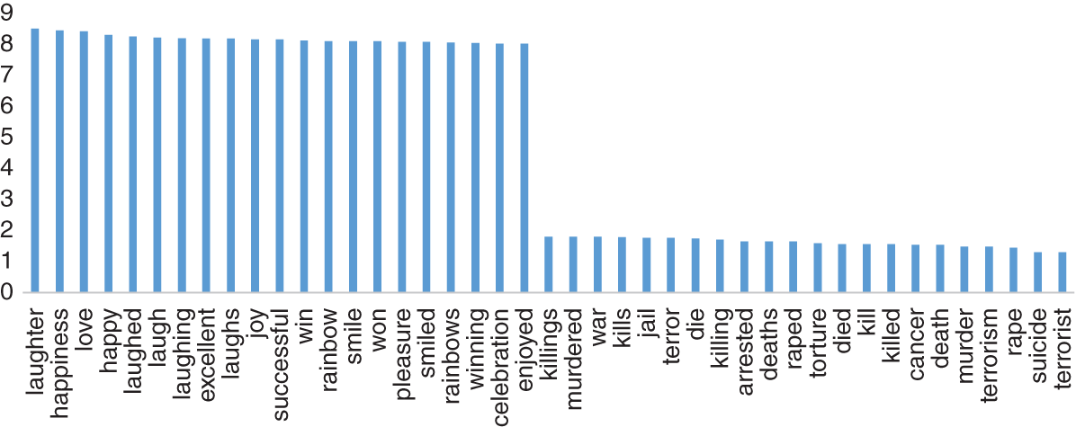
FIGURE 15.1 Happiest and saddest words in Hedonometer's corpus.
Source: Based on data from Hedonometer.
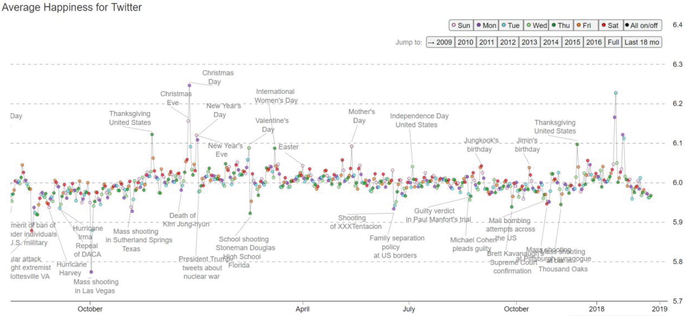
FIGURE 15.2 Hedonometer index for latter part of 2018 till early 2019.
Source: Hedonometer.
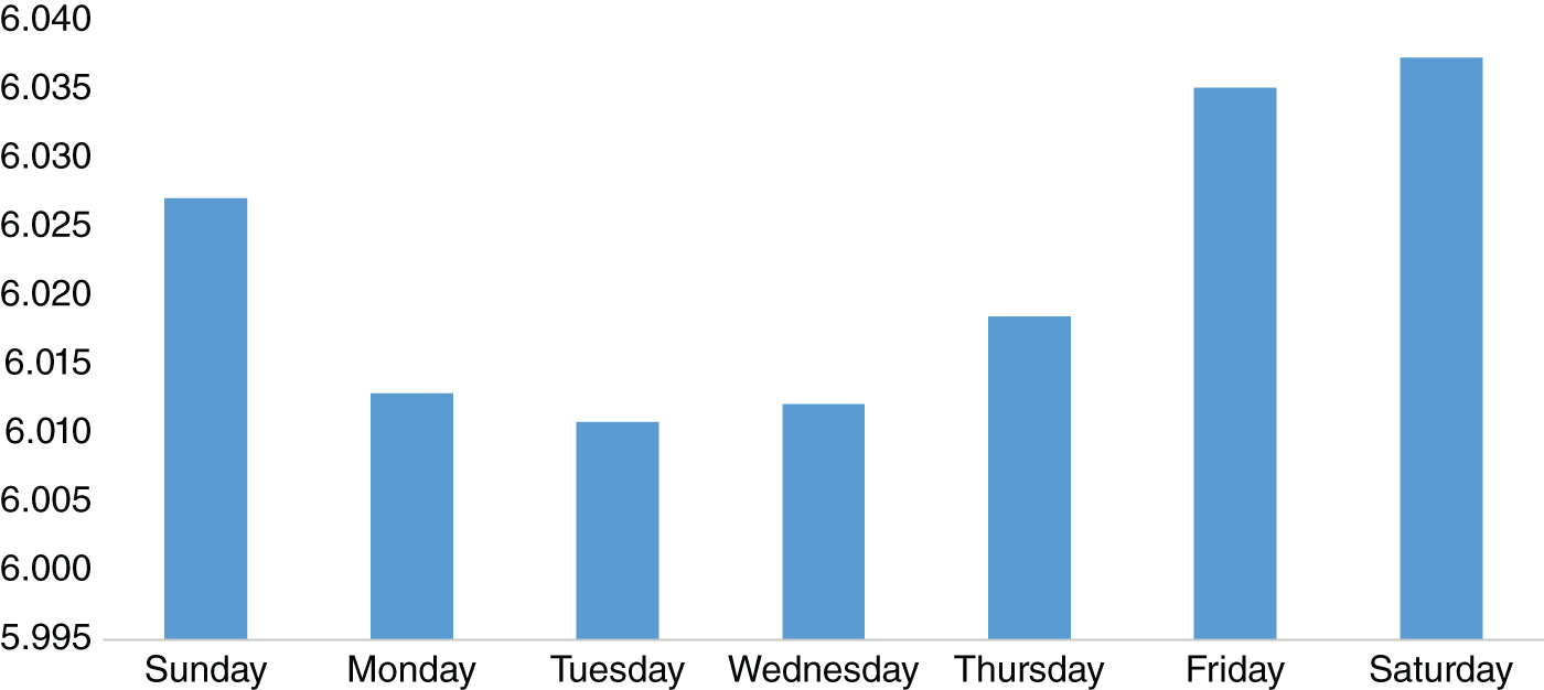
FIGURE 15.3 Average Hedonometer score by day of the week.
Source: Based on data from Hedonometer.
Can we make a connection between happiness and markets? After all, we would think that overall consumer confidence would be linked to happiness, and hence it could be a reasonable indicator for risk sentiment. In order to do this, we created the HSI (Happiness Sentiment Index) out of the Hedonometer Index. This first step involves stripping out weekends, given they are non-trading days. We also exclude outlier days (i.e. where there are significant jumps in the Hedonometer index, which we have defined at moves greater than 0.05). Furthermore, we exclude any US holidays, where people are generally likely to be happier; otherwise our model will simply be biased to suggesting good market sentiment because of holidays rather than for any other reason. Indeed, we already observed, for example, that the Hedonometer index is highest during the weekend.
A 1-month SMA is then applied to smooth the index. Finally, the scores are standardized between 0 and 1, using a rolling percentile rank with a 2-month window. Figure 15.4 plots the HSI against the 1-month changes in S&P 500 1st dated futures. At least from this specific example, there does appear to be somewhat of a relationship between moves in the S&P 500. If we regress the HSI against S&P 500 during our sample (February 2009–July 2019), the T-statistic of the beta coefficient is 7.7 (and has p value of 2.13*10^-14), which shows a statistically significant relationship between S&P 500 and HSI. This suggests that the HSI could potentially be used as an indicator for trading markets. In practice, of course, it is likely that it would be combined with a number of other market sentiment metrics, which could, for example, include news sentiment or market positioning.
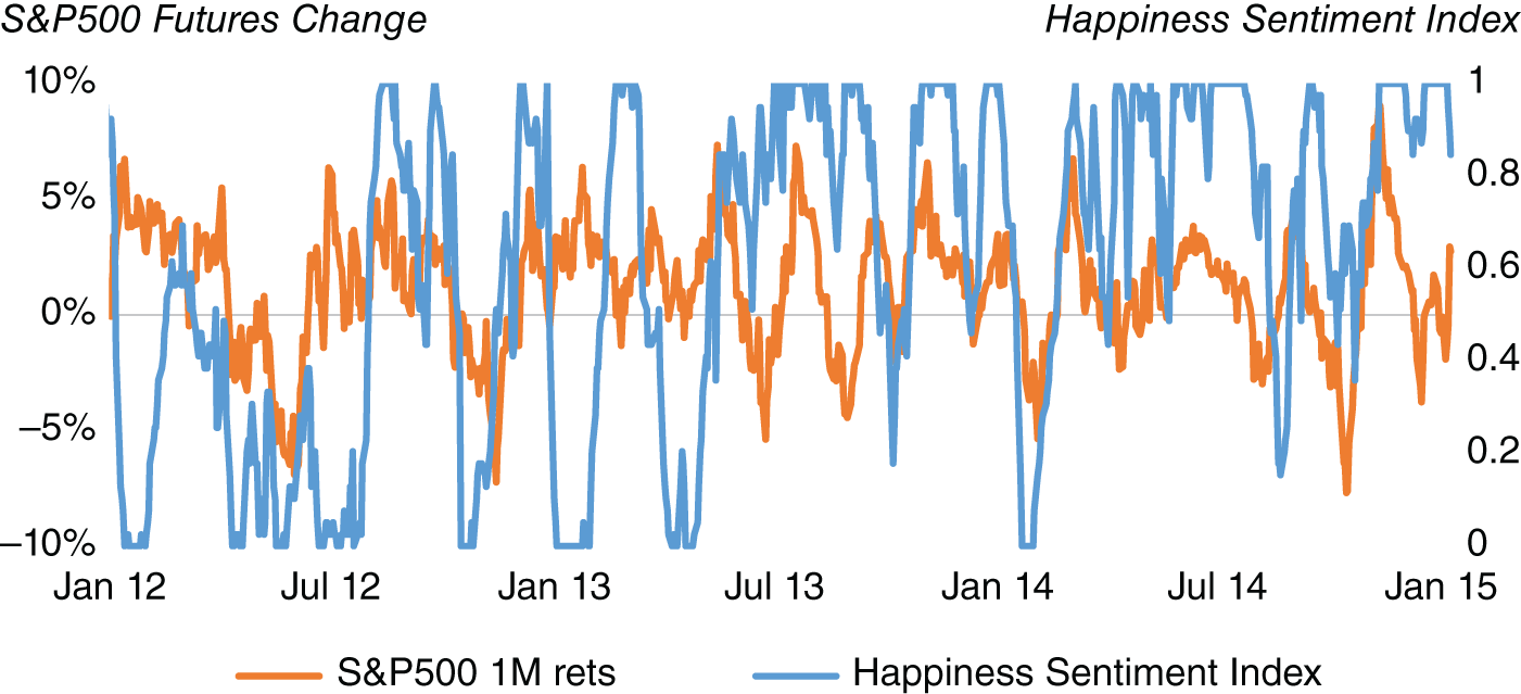
FIGURE 15.4 Happiness Sentiment Index against S&P 500.
Source: Based on data from Hedonometer Index, Bloomberg.
15.3.2. Using Twitter Data to Help Forecast US Change in Nonfarm Payrolls
We have seen that we can derive an indicator that gives a representation for the happiness of Twitter users from their tweets. Are there very specific ways we can use Twitter to help us understand the market? Social media gives us an idea of what people are talking about at any specific moment. Hence, it seems reasonable to assume that they might be able to give us insights into the economy at any particular time. One of the most keenly awaited economics releases is the US employment situation report, which usually happens on the first Friday of the month from the US BLS (Bureau of Labor Statistics) at 8:30 am EST. The report relates to the jobs market in the previous month. It is usually the first official release of actual “hard” US economic data in the month. Before that, much of the data tends to be “soft” data or from surveys based upon people's expectation about the economy. There is also the privately compiled ADP employment report, which is published before the BLS data, but the market tends to place less weight on its release.
The US employment situation report contains a number of different statistics relating to the labor market (Bureau of Labor Statistics, 2019), which are broken down into two parts: the household survey of around 60,000 households and the establishment surveys of businesses (around 142,000).
The statistics that are the most relevant to the market are the national unemployment rate (from the household survey) and the national monthly change in nonfarm payrolls (from the establishment survey). Market expectations for nonfarm payrolls are typically determined by consensus surveys (such as those conducted by Bloomberg) of US economists working in large financial institutions.
As the name suggests, nonfarm payrolls omit farm workers. Historically, measures of farm labor are collected by the US Department of Agriculture's Census of Agriculture. The release of the US employment situation report also includes revisions to the previous estimates, as well as many other statistics, such as average hours worked, earnings, and the participation rate. In many cases, there is a significant amount of granularity available in the underlying statistics, sometimes down to state level and subsectors. Indeed, at the time of publishing, ALFRED (n.d.) has over 8,500 time series sourced from the household survey and 811 time series sourced from the establishment survey.
There is usually a very strong relationship between the surprise in the change in nonfarm payrolls on the one hand, and the move in US Treasury yields and the move in the USD on the other. The rationale is that when economic data is stronger, it is more likely that FOMC will adopt a hawkish tone and yields will climb higher to reflect that. The converse is true when data is weaker. Typically, the USD also reacts in this way, moving with US Treasury yields after strong data. There have been occasions in the past, however – for example, following the financial crisis – that the USD actually strengthened after very poor payrolls releases. One rationale was that investors were flocking toward USD as a flight-to-safety trade given its status as the main reserve currency.
To illustrate this, in Figure 15.5 we plot the surprise in nonfarm payrolls between 2011 and 2016 versus the returns in USD/JPY in the 1 minute following the release of the US employment report. The surprise is simply the actual released number minus the consensus number. We note that with very large surprises the reaction tends to be nonlinear. When the surprise is positive then USD/JPY tends to move higher, and when it is negative it tends to move lower, which seems fairly intuitive for the reasons we have discussed.
Hence, if we could forecast the “actual” change in nonfarm payrolls better than consensus, we could potentially monetize it by entering the trade before 8:30 am EST on the day of the US employment situation report and exiting it shortly after. In other words, if our more accurate forecast was higher than consensus, we would buy USD; conversely, we would sell USD if our forecast was lower. As traders, our objective is not necessarily to minimize the standard error of our forecast, but instead to generate alpha from a forecast. If a forecast has a smaller standard error but misjudges the direction of an event surprise, often it is of less use for a trader.
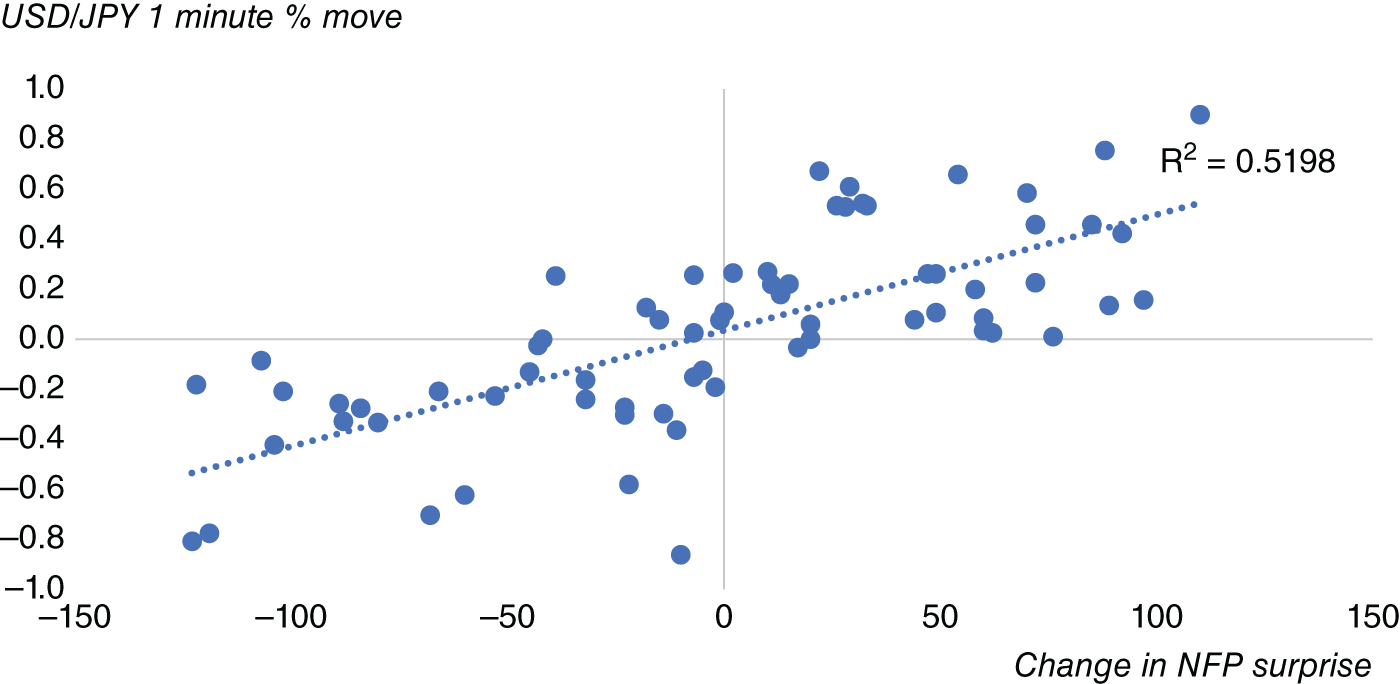
FIGURE 15.5 Surprise in nonfarm payrolls vs. USD/JPY 1-minute move after release.
Source: Based on data from Bloomberg.

FIGURE 15.6 Twitter-based forecast for US change in nonfarm payrolls versus actual release & Bloomberg consensus survey.
Source: Based on data from Twitter, Bloomberg.
Note that we are not trying to use some sort of latency advantage attempting to be the first one to trade immediately after the release. There is likely to be very little liquidity at that time, and furthermore we would have to have very sophisticated and expensive technology to be able to engage in this type of latency arbitrage. So how can we try to get a more accurate forecast for payrolls? One approach can be to augment existing variables we use to forecast payrolls (typically related to variables that use existing labor market data). In our case, we shall attempt to use data derived from tweets related to chatter about the labor market as an additional Twitter variable to augment our model. Figure 15.6 plots our Twitter-enhanced payrolls model forecast alongside the first release of nonfarm payrolls and also the consensus survey of economist estimates from Bloomberg. Our model-based nowcast is available on a daily basis, given that we can have access to Twitter data on a high-frequency basis. Our sample is again from early 2011 to summer 2016. We see that there are certain periods where our model-based nowcast managed to pick up the actual NFP number very well, such as at the start of 2014, despite the survey number being way off. However, purely from this plot it is difficult to tell on aggregate whether you could trade our model NFP forecast profitably. In order to understand that, we need to do more work and backtest a trading strategy.
Basically, how useful is this enhanced nowcast for nonfarm payrolls for a trader? We can check this historically by doing a backtest using a very simple trading rule, which we described earlier:
- Buying USD when our estimate is better/higher than consensus
- Selling USD when our estimate is worse/lower than consensus
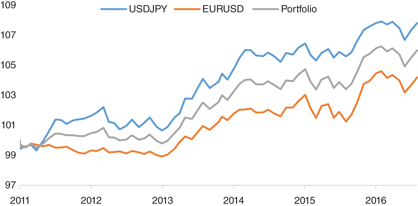
FIGURE 15.7 Trading EUR/USD and USD/JPY on an intraday basis around NFP.
Source: Based on data from Twitter, Bloomberg.
In Figure 15.7, we use our enhanced forecast to trade EUR/USD and USD/JPY on an intraday basis around payrolls, entering the trade a few minutes before the data release and exiting a few minutes after. The average returns on an annualized basis are 119 bps for USD/JPY and 59 bps for EUR/USD. An equally weighted portfolio of EUR/USD and USD/JPY has average return of 88 bps. Obviously, there are some major caveats to this type of analysis, given that our sample is relatively small. Indeed, we only have 68 data releases in our sample. Furthermore, we have to bear in mind that we would need access to good liquidity to execute such a strategy. With wider spreads, it would be difficult to monetize such a trading rule.
15.3.3. Twitter Data to Forecast Stock Market Reaction to FOMC
We have noted that Twitter can be used to improve forecasts for nonfarm payrolls. However, can it be used in other ways? Azar and Lo (2016), for example, discuss how to use tweets to forecast future returns around FOMC. The approach requires the filtering of tweets in the runup to FOMC meetings, specifically filtering on terms “FOMC” and “Federal Reserve” and the name of the Fed chair during their historical sample of 2007–2014 (i.e. “Bernanke,” later “Yellen,” and so on). Basic sentiment analysis was applied to each tweet, to give a score between –1 and +1 using a deterministic algorithm, dubbed “Pattern,” which relies on a database containing positive/negative scores for each word. It also takes into account the use of adjectives and adverbs to “amplify” or “dampen” the score. Hence, it should capture that “not good” exhibits a negative sentiment. These scores are then weighted by the number of followers of the user tweeting. These weighted scores are aggregated into daily sentiment scores. In practice, the historical sample was curtailed to 2009–2014, given the relatively small volume of tweets in their sample between 2007 and 2009. The authors construct various portfolios that incorporate this sentiment information from tweets and then compare it to a market benchmark portfolio. They note that a model that includes these tweets – in particular immediately preceding an FOMC meeting – performs well. Just as with the example showing a trading rule applied to the US employment situation, we need to note that there are a relatively small number of FOMC meetings in the sample. Potentially, one way to increase the sample space could be to apply the same approach to other central banks, such as ECB or BoJ and examine whether tweets provide informational content for the reaction of domestic assets such as bonds and equities. To our knowledge, this has not been attempted yet.
15.3.4. Liquidity and Sentiment from Social Media
We have already given some examples of why understanding sentiment is an important component of trading. When sentiment is negative and hence the market becomes more risk averse, we might expect liquidity to be more constrained. Essentially, market makers need to be compensated for offering liquidity in environments where traders are scaling back their risk exposure. In contrast, when sentiment is good, we might expect liquidity to be more abundant and we should find it easier to transact. Agrawal, Azar, Lo, and Singh (2018) discuss the relationship between social media sentiment and equities market liquidity. To measure social media sentiment, they use a feed from PsychSignal that supplies a time series of sentiment scores related to equities based upon data from Twitter and Stocktwits. They compare this against a feed of sentiment scores from RavenPack's news dataset. They show that negative sentiment based on social media tends to have a bigger impact on liquidity than positive sentiment. They find that highly abnormal social media sentiment tends to be preceded by high momentum and this is followed by a period of mean-reversion. Using some of these observations they develop some equities-based trading strategies that use social media as an input and that outperform their benchmark with the caveat that their relatively high frequency makes them amenable only for those with access to lower transaction costs.
In terms of further study, they note that overall it can be difficult to identify the direction of causality in their study. Do price moves drive social media, or vice versa? They also note that not all social media users have the same impact, which seems entirely intuitive in particular, given the disparity in followers and general influence.
15.4. NEWS
News has always had an impact on markets and it is very much a traditional source of information. However, what has changed is that the volume of news has grown significantly over the years. In Figure 15.8, we illustrate this by plotting S&P 500 against the number of stories on Bloomberg News, whose text includes S&P 500. We note that in the late 1990s, the story counts were less than half where they are today. In this instance, we are examining a single source of news (Bloomberg News). In recent years the number of sources of news has also increased significantly, largely due to the web. It is clearly impossible for one human to read every single news article published about the market. However, what if that reader of news was not a human?
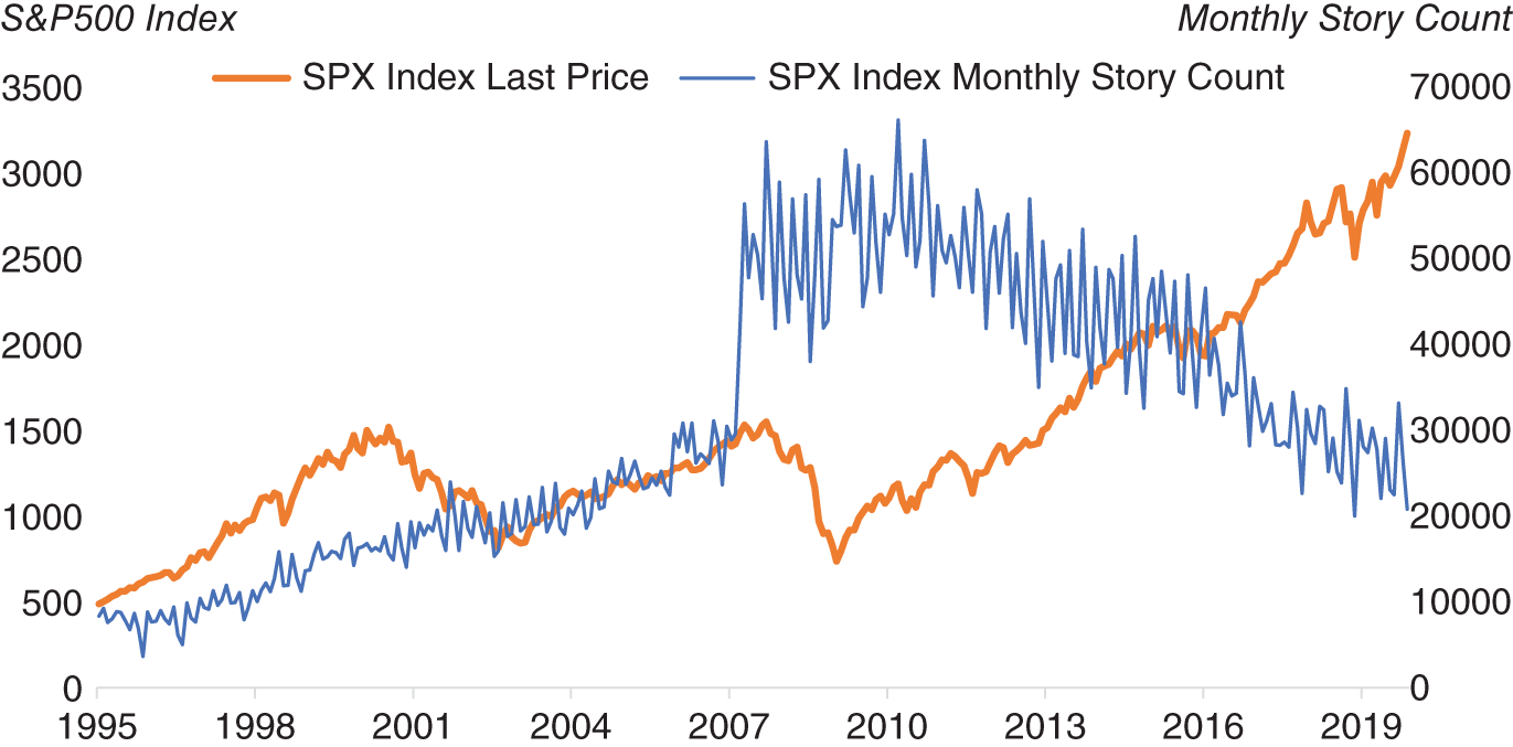
FIGURE 15.8 S&P 500 versus article count on it on Bloomberg News.
Source: Based on data from Bloomberg.
Recently, newswires that have been traditionally read by traders on their computers through proprietary applications, such as Bloomberg News, have begun to be distributed in machine-readable form. As the name suggests, news that is in a machine-readable form can be parsed by a computer. Typically, machine-readable news published by newswires will already have a large amount of structure, which makes it easier to discern content in them. Furthermore, vendors will typically add a significant amount of metadata, such as the topic of news article, its sentiment, and the entities referred to in the text. In addition, it will be written in a relatively consistent style.
A large amount of news is obviously also published on the web, both by traditional news outlets and in other forms such as blogs. We could also argue that a lot of social media itself is informed by news articles. In practice, web-based content gathered from disparate sources requires a significant amount of structuring into an appropriate and consistent form before it can be made into a form that is usable by traders. Other important sources of text data for markets include material published by companies about themselves, such as corporate call transcripts and interviews.
For high-frequency traders, a computer can obviously parse text and interpret it much more quickly than a human, and hence react faster. For longer-term strategies, automated parsing is also beneficial, allowing the parsing of vast amounts of news that can be aggregated together to give a more rounded view of what is being reported in the press.
15.4.1. Machine-Readable News to Trade FX and Understand FX Volatility
We have noted the general rationale behind using machine-readable news to understand and hence predict markets. A use case that we will examine in this section is how to extract sentiment from news to generate signals to trade FX from a directional perspective. Amen (2018) discusses how machine-readable news from Bloomberg News (newswire between 2009 and 2017) can be used to create sentiment scores for G10/developed market currencies. We will give a brief summary of the paper here and will illustrate its results. The rationale for using machine-readable news is that historically news has always been a key part of the decision-making process for traders. The dataset is structured such that each record has the time stamp of each news article as well as other fields, such as topic and ticker tags. The dataset is then filtered in a way that only articles related to each developed market currency are read. In Figure 15.9, we give the average daily number of news articles for each currency from the paper. We note that the most heavily traded currencies, such as EUR and USD, have more news articles as we would expect.
Amen (2018) applies natural language processing to each of these articles to ascertain the sentiment score. We need to be careful in understanding FX quotation conventions, which can sometimes require us to flip the score. For example, if we are trying to capture sentiment for JPY, and the currency pair is quoted in USD/JPY, we would need to invert the score. We calculate a daily sentiment score by creating a cutoff point at 5 pm EST each day and calculating an equally weighted average of all the sentiment scores for that currency over the past day. We then construct a Z score (![]() ) for each daily observation (
) for each daily observation (![]() ) by subtracting the mean of the daily observations (
) by subtracting the mean of the daily observations (![]() ) and dividing by the standard deviation of the daily observations (
) and dividing by the standard deviation of the daily observations (![]() ). The mean and standard deviation of the daily observations are calculated over a rolling window. The Z score normalizes sentiment across different currencies.
). The mean and standard deviation of the daily observations are calculated over a rolling window. The Z score normalizes sentiment across different currencies.
We now have scores for each currency. To construct a score for a particular currency pair, we simply subtract one from the other. For example, the USD/JPY score is simply USD – JPY. We plot this specific metric in Figure 15.10 alongside weekly returns.
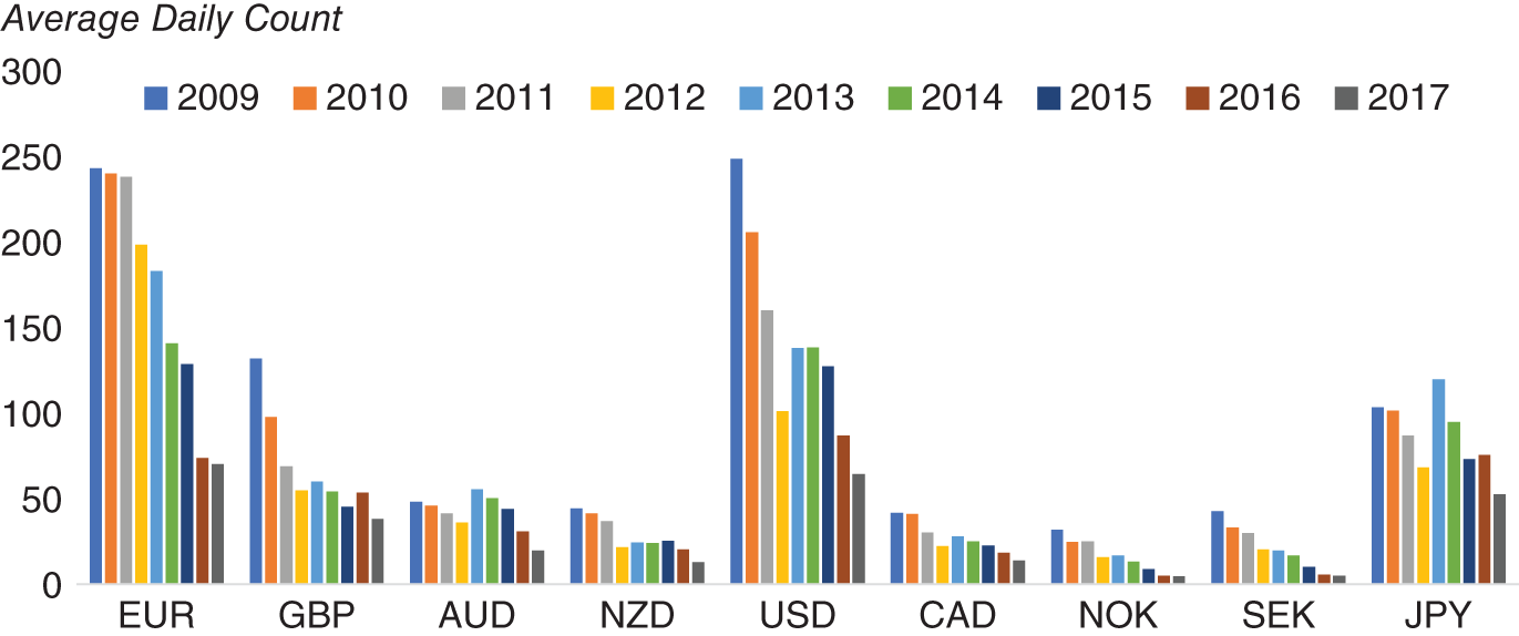
FIGURE 15.9 Average daily count of articles per ticker.
Source: Based on data from Cuemacro, Bloomberg.
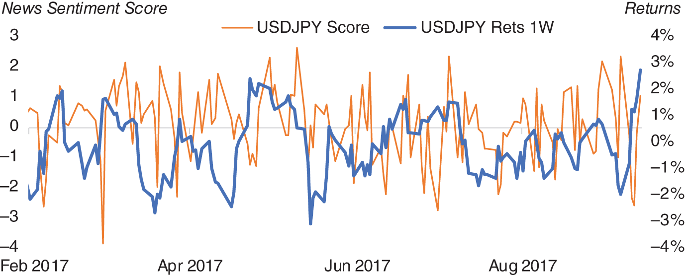
FIGURE 15.10 USD/JPY news sentiment score versus weekly returns.
Source: Based on data from Cuemacro, Bloomberg.
We now have a way of identifying the sentiment for any particular developed market currency pair from underlying news data. We can apply a simple trading rule, buying that currency pair when the sentiment is positive and selling when it is negative. Of course, this approach of trading with the short-term momentum in the news is just one approach to using news data. Another approach could involve looking at news data over extended periods and then fading extremes as follows. When there is very good news over a prolonged period of time, the market will tend to be conditioned to it. The market has basically already priced in “good news” in such a scenario. Hence typically the market will not react so positively to it. Conversely, if we see something similar with extremely bad news, after a while the market becomes used to it and has priced it in. Hence, it no longer reacts negatively. We might even see the market bounce.
Does such a short-term news momentum trading rule, as described here, work in practice? We can backtest this trading rule using historical data. The risk-adjusted returns (i.e. information ratios) for this trading strategy for each currency pair are presented in Figure 15.11 alongside returns for a generic trend-following strategy on price data, which is one of the typical strategies used by FX traders historically. We see that while trend following has underperformed in our sample, our news-based approach has been profitable. In Figure 15.12 we plot the correlation between the returns of these two strategies for each currency pair. We note that there is no consistent pattern, suggesting that the factor we are extracting from news adds value to a trend-following strategy on prices.
We can also construct a basket of all these currency pairs using both our news-based and trend-following trading rules. In Figure 15.13, we present the returns of these baskets. As we would expect from our earlier currency pair–specific example, the news-based basket outperforms trend (risk-adjusted returns of 0.6 versus –0.3 respectively). In Figure 15.14, we show the year-on-year returns of both baskets. In most years, news outperforms, with the largest exception being 2010, where news heavily underperforms trend.
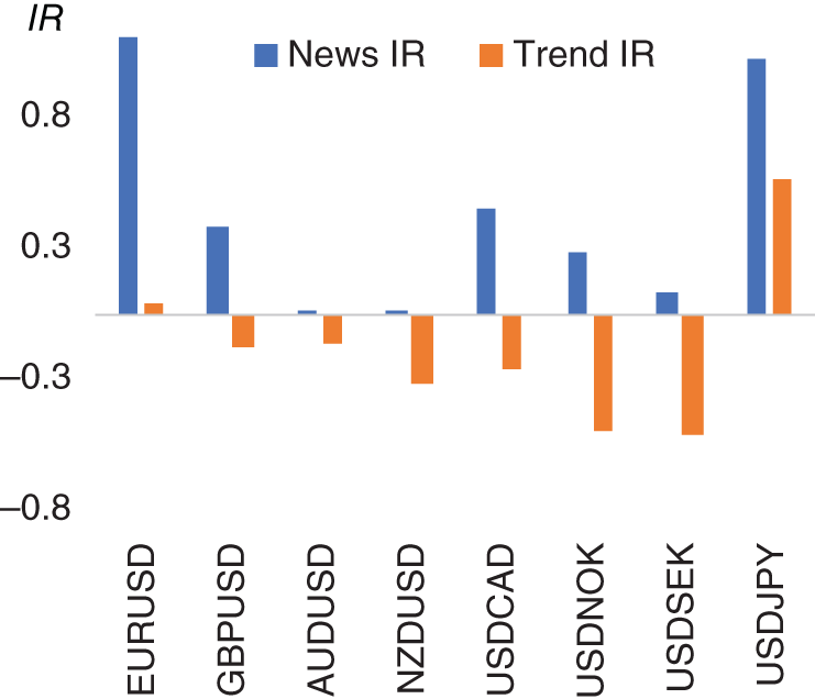
FIGURE 15.11 News versus trend information ratio.
Source: Based on data from Cuemacro, Bloomberg.
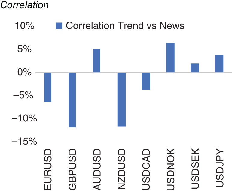
FIGURE 15.12 News versus trend correlation.
Source: Based on data from Cuemacro, Bloomberg
Another way we can extract value from news data is to understand how it can be used to understand FX volatility. Amen (2018) also shows how news volume on a certain asset can have a strong contemporaneous relationship with the volatility of that asset. In Figure 15.15, we see the news volume on USD/JPY plotted against the news volume score, which is essentially a standardized metric relating to the news volume on articles tagged in the Bloomberg News (BN) newswire as relating to USD/JPY. At least from this single plot, it does appear that there is some link between news volume and volatility. This is of course intuitive – that there is more news written about an asset that is exhibiting more volatile price action.
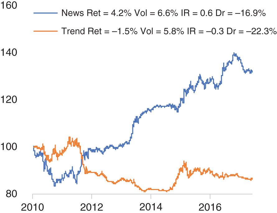
FIGURE 15.13 News versus trend model returns.
Source: Based on data from Cuemacro, Bloomberg.
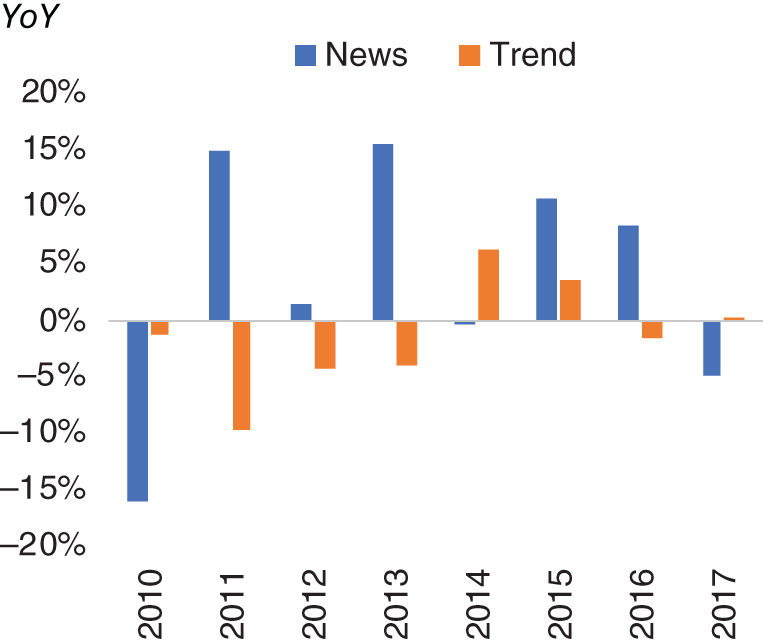
FIGURE 15.14 News versus trend model YoY returns.
Source: Based on data from Cuemacro, Bloomberg.
In Figure 15.16, we report the T-statistics from a regression of daily returns against the news volume metric for that same currency pair using the same historical sample 2011–2017. We see that in every case (other than USD/NOK), the T-statistics are statistically significant, confirming our intuition that volatility and news volume are strongly linked. All the p-values are well below 0.05 (other than USD/NOK, which is 0.27), indicating statistical significance.
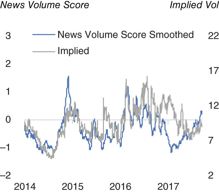
FIGURE 15.15 USD/JPY news volume versus 1M implied volatility.
Source: Based on data from Cuemacro, Bloomberg.
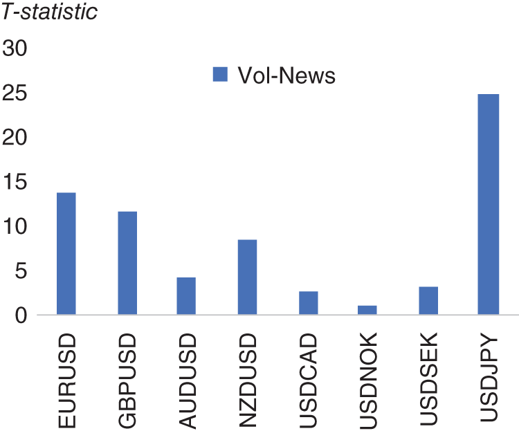
FIGURE 15.16 Regressing news volume versus 1M implied volatility.
Source: Based on data from Cuemacro, Bloomberg.
Are there potentially other ways we can utilize the observation that news volume is linked to volatility? One way is to understand the volatility around major scheduled events such as FOMC and ECB meetings. Obviously, before a scheduled economic event, there is no certainly concerning the outcome, but we do at least know the timing. Hence, before these meetings, volatility traders will typically mark up implied vol, given the expectation of heightened realized volatility over these events. This additional markup is typically known at the event volatility add-on and is expressed in terms of overnight volatility. For events like central bank meetings, the event vol add-on can be substantial. For lesser events, the event vol add-on can often be negligible.
In Figure 15.17, we plot the overnight implied volatility for EUR/USD just before an FOMC meeting, ignoring all other days (hence the option would expire just after FOMC). We also plot the add-on associated with EUR/USD ON, which has been generated by a simple model. Alongside this we plot the subsequent realized volatility on FOMC days and the volatility risk premium (VRP), which is simply implied minus realized volatility. Our first observation is that the implied volatility is nearly always more than realized volatility on FOMC days. This shouldn't be surprising, given that traders need to be compensated for selling “insurance.” Typically, the times when buying options is profitable are during Black Swan events, when both the timing and the nature of the event are totally unpredictable. It can be argued that events like FOMC are not really Black Swan events, given that we at least know the timing. The add-ons are typically around 4 volatility points. In other words, EUR/USD overnight implied volatility is around 4 volatility points higher just before FOMC meetings.
However, what can news tell us about EUR/USD overnight implied volatility before FOMC meetings? One way to see this is to look at the normalized volume of FOMC articles on Bloomberg News, in the days in the runup to an FOMC meeting (we obviously ignore news articles written after FOMC). In Figure 15.18, we plot EUR/USD overnight implied volatility just before FOMC meetings against this normalized news volume measure. At least on a stylized basis there does appear to be some sort of relationship between the news volume on FOMC before a meeting and how volatility traders price implied volatility. This should seem intuitive. If there is a lot of chatter about a particular FOMC meeting, there are more expectations of significant policy changes (and hence volatility). Conversely when there is little chatter, it would suggest that the FOMC meeting is likely to be relatively quiet.
We can view the data in another way using scatter charts (see Figure 15.19). These charts show the normalized FOMC volume against the add-on, implied vol, and realized vol of EUR/USD. We also report the ![]() of these regressions. The
of these regressions. The ![]() are not negligible in all instances. This suggests that potentially using news volume as an indicator could be a useful addition when modeling volatility over major scheduled events.
are not negligible in all instances. This suggests that potentially using news volume as an indicator could be a useful addition when modeling volatility over major scheduled events.
The exercise can also be repeated for examining EUR/USD overnight volatility before ECB meetings (see Figure 15.20). We see a similar picture as we did for FOMC.
15.4.2. Federal Reserve Communications and US Treasury Yields
Historically, central banks have not always been open with how they operate. Indeed, Bernanke (2007) notes that Montagu Norman, the governor of the Bank of England from 1921 to 1944, had a personal motto: “Never explain, never excuse.” However, as a whole, central banks have become far more open in the decades since that era. As Bernanke stresses, ultimately central bankers are public servants and their decisions can have a big impact on society. Thus, they have a responsibility to explain the rationale behind their decisions.
The Federal Reserve communicates in a number of different ways. The FOMC (Federal Open Markets Committee) consists of 12 members who vote on Fed policy. All seven members of the Board of Governors of the Federal Reserve System and the president of the Federal Reserve Bank of New York are permanent members of the FOMC. The other four alternate members are chosen from the other 11 Reserve Bank presidents who serve rotating one-year terms. As noted in Chapter 9, nonvoting Reserve Bank presidents still take part in meetings of the FOMC and all the various discussions concerning Fed policy, as well as contribute to the Fed's assessment of economic conditions.
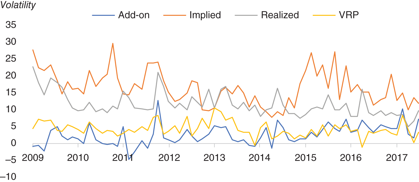
FIGURE 15.17 EUR/USD ON volatility add-on, implied volatility, realized volatility, and volatility risk premium (VRP) on FOMC days.
Source: Based on data from Cuemacro, Bloomberg.
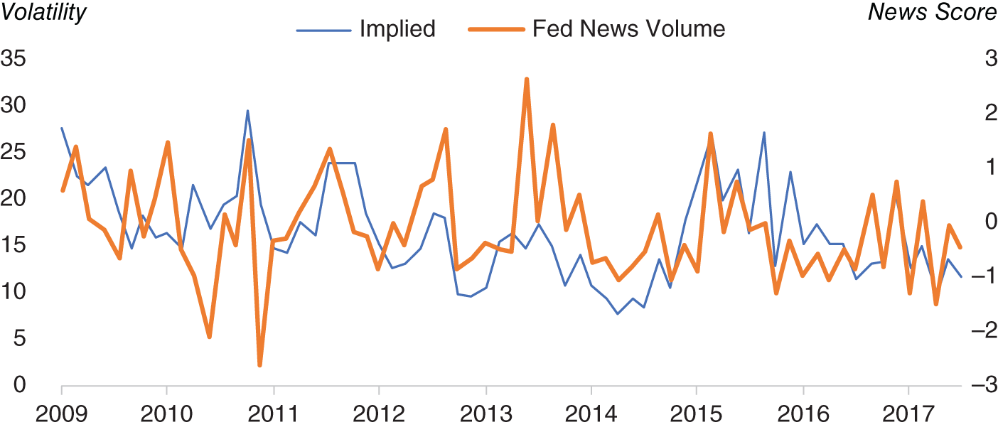
FIGURE 15.18 EUR/USD ON implied volatility on FOMC days against FOMC news volume.
Source: Based on data from Cuemacro, Bloomberg.
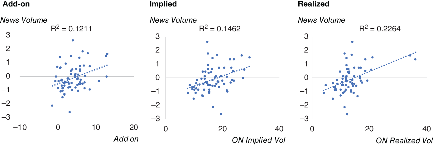
FIGURE 15.19 EUR/USD overnight volatility on FOMC days.
Source: Based on data from Cuemacro, Bloomberg.
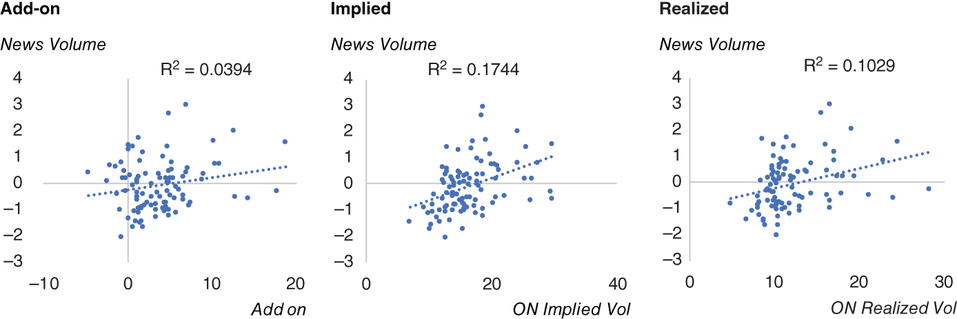
FIGURE 15.20 EUR/USD overnight volatility on ECB days.
Source: Based on data from Cuemacro, Bloomberg.
Communications from the FOMC can involve the statements and press conferences that accompany each FOMC meeting (of which there are 8 every year) where monetary policy changes can be made. There are also more detailed minutes that give further insights into the decision-making process, which are published several weeks after each meeting. Transcripts of FOMC meetings are published several years afterwards. While they might not be relevant from a market perspective, they nevertheless shed light on the general workings of the Fed. Voting members of the FOMC and nonvoting members also regularly give speeches to the public, sometimes concerning monetary policy and other subjects under the remit of the Fed, such as regulation. They also regularly appear in the media on TV, radio, in the press, and also even sometimes tweeting from their own social media accounts. Typically, market participants collectively refer to communications from the Fed as Fedspeak.
If the Fed becomes more hawkish, suggesting that it might have to increase the base rate, then we might expect yields in the front end of the US Treasury curve to rise. Conversely, if their communications are pessimistic about growth and expect inflation to fall, suggesting a more dovish outlook, we might expect front-end yields to fall. In a sense, we can view bond yields as proxies for monetary policy expectations, in particular those without significant credit exposure, such as US Treasury yields. In recent years, through quantitative easing, the Fed has also had a larger impact further along the yield curve.
As a result, for market practitioners, trying to understand how the Fed sees the economy and an understanding of how it views future monetary policy is crucial. Historically, economists have pored over Fed communications to see if they can glean an idea of future policy. Ultimately, the Fed, like everyone else, cannot see the future with perfect foresight. However, the Fed does have the power to change monetary policy.
The annual volume of communications from the FOMC, while it might encompass many pages of text, is ultimately “small data,” which could comfortably fit in a few megabytes. So theoretically, it is possible for an economist to read a large amount of this text, if they are a “Fed watcher.” However, in practice, many market participants will likely skim through only a small number of communications at best.
A large amount of FOMC communications is available from the various Fed websites, although some might only be available to subscribers of various news organizations. Hence, we can get a reasonable corpus of FOMC communications by parsing a number of websites. What steps need to be taken in order to do this?
In practice, we first need to do a substantial amount of work. We need to identify the specific web pages that have Fed communications. It is necessary to structure the raw text downloaded, so we dispense with HTML tags and the like and only capture the body text of the article. Once we have extracted the raw text, we can present that alongside metadata, such as the speaker and the time stamp of the communication. As a further step, we can use additional metadata related to sentiment for each communication. As a final step, we can create an index of the various sentiment scores. This will give us an idea of the general path of Fed communications, which can be useful from a longer-term trading perspective.
We are essentially “structuring” the Fed communications into a time series that is more easily interpretable by traders. So, after we have done all of this work, would such an index actually help us understand the moves in US Treasury yields?
In Figure 15.21, we have plotted Cuemacro's Fed communications index between 2015 and 2017, which has largely been constructed in the way we described, only using text as an input, and no other market variables such as bond yields, equity moves, and so on. While it does not encompass absolutely every single example of Fedspeak, it does capture a large proportion of it and in particular the various statements, press conferences, and minutes, as well as many of the speeches. Alongside the index, we have also plotted the 1M change in US Treasury 10Y yields. Note that we discuss the various aspects of the Fed communications in a large amount of detail in Chapter 9, in particular discussing ways of detecting outliers from a preliminary version of the dataset of Fed communications used in Cuemacro's Fed communication index.
We note that for the most part, at least from a stylistic perspective, there does appear to be a relationship between the two time series. If we do a linear regression of the Fed communications index and 1M change in US Treasury 10Y yields, using a sample between 2013 and 2019, the T-statistic of the beta of the regression is close to 4.8 with a p-value of 1.2*10^-6, suggesting a statistically significant relationship between them. The correlation is around 11% during this same sample.
It is, of course, intuitive that there is a relationship between the sentiment of the Fed and moves in UST 10Y yields for the reasons we discussed earlier. We note there are periods in time where there are significant divergences between the Fed communications index here and the moves in UST 10Y yields. In particular, during November 2016, there was a significant rise in UST 10Y yields going against the move in the index. In this instance, bond yields were reacting more to the election of Donald Trump and the whole theme of “reflation” rather than the underlying message from the Fed. This, of course, illustrates that markets move for many different reasons, and it is difficult to isolate a single factor that will always drive price action.
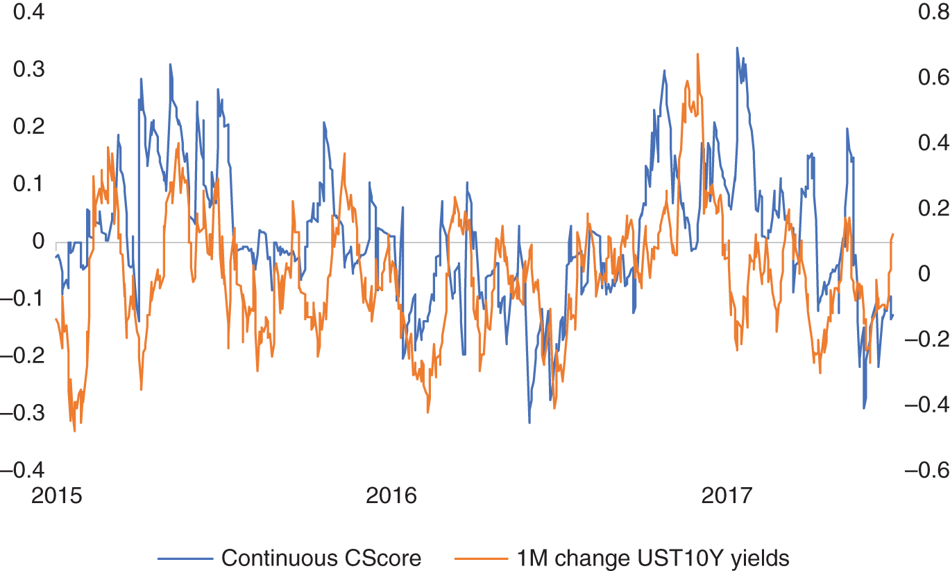
FIGURE 15.21 FOMC sentiment index and UST 10Y yield changes over the past month from 2015 to 2017.
Source: Based on data from Cuemacro, Federal Reserve.
15.5. OTHER WEB SOURCES
The web obviously contains a large body of information that does not fall under either news or social media. There is also a substantial amount of content published on the web by individuals such as blogs. Corporate institutions also publish a large amount of data as part of their everyday business – for example, to promote themselves and also to interact with their clients, such as online retailers. Given the huge amount of data available on the web, it is likely that we can structure some relatively unique datasets from it.
We can use these other forms of web data to gain insights into financial markets. There are a number of data vendors focused on structuring data relevant for traders from the web, such as Import.io and ThinkNum. We can derive jobs data from the web. We can monitor corporate websites for current job openings data to get a specific picture on hiring by company. Expanding companies are likely to have more job openings. The health of a company can also be gauged by tracking store openings and closings that can be derived from web data. It is also possible to gauge consumer sentiment toward brands by looking at forum postings.
For many sectors there might not be “traditional datasets,” and hence our only recourse is to use web-sourced datasets. For example, there are published metrics relating to the hotel industry, which give us an idea of the average daily rate, the revenue per available room, inventory, and so on. However, for location rentals that have recently been popularized by firms such as Airbnb, it is difficult to source such information. One solution is to derive these metrics from web data.
Next we discuss using data derived from online retailers to generate high-frequency inflation measures. We can derive many other datasets from websites for online retailers, aside from inflation. We can also get an idea of real-time inventory for products stocked by them. This can be particularly useful for product sectors where there are not similar existing datasets, and even for those where we have data it often is not as timely. Over time data history can be built up to construct time series of many of these web-sourced metrics. Having a longer time series can help with backtesting and understanding the effectiveness of the signal historically.
15.5.1. Measuring Consumer Price Inflation
Cavallo and Rigobon (2016) discuss using online prices to improve the understanding of consumer inflation, which they called “The Billion Prices Project.” Consumer inflation price indices have typically been calculated by national statistics on a monthly or bi-monthly basis. It involves monitoring the price of a basket of goods and recording its changes. This data is collected manually by people from national statistics agencies visiting hundreds of stores. Over time the basket changes, as consumer preferences change. This data is aggregated into the consumer price indices.
Today, a large number of consumer transactions now occur online. In certain countries, official inflation data might be very unreliable or even simply not released, as Cavallo and Rigobon (2016) note for much of the period 2007–2015 in Argentina. Hence, it can be important to find alternative ways to measure consumer price inflation. Even for those countries where data is released regularly and is considered reliable by market participants, we might also wish to have a higher-frequency measure. It might also be useful in estimating the official release of inflation data and help us in trading decisions.
The prices of products sold by retailers can be scraped in a relatively automated way, as opposed to the traditional manual process of visiting shops, providing a much larger sample of price changes at a micro level. This is conditional on the items being relatively consistent over time. For example, we might have the situation where brands maintain the same price of their products but reduce their quality or size. One example of this is reducing the size of chocolate bars while maintaining the same price.
This data can then be aggregated into higher-frequency consumer inflation indices, which fit closely with many official time series. It is also possible to understand relative price levels across different countries with a different aggregation of the micro level information of similar products, which you cannot do by comparing consumer price indexes themselves. The authors give a specific example of products available globally, like those from Apple, IKEA, Zara, and H&M, which can be used to create such a consumer goods basket across different countries. The Big Mac Index, published by the Economist, attempts to do something similar, but of course just by examining a single item, the humble McDonald's Big Mac, and is more for illustrative purposes a PPP (purchasing power parity) model for estimating the long-term valuation of currencies. “The Billion Prices Project” evolved into a commercial entity, PriceStats, now owned by State Street, which distributes consumer inflation indices generated using this online approach on a daily basis.
15.6. SUMMARY
We have noted that the use of text to help traders make decisions is not new. However, what is new is that the amount of text available for investors has mushroomed in recent years. This is driven in large part by the advent of the web. Text can come in many different forms, ranging from newswire stories to social media and in many other forms, including the web pages of corporates. The sheer volume means that automated techniques are required to make sense of it all. Once structured and aggregated this text data3 can be used to help inform the decisions of traders.
We have shown specific text examples, like using the social media chatter around labor markets to help forecast the change in US nonfarm payrolls. We have shown how to use the tone of social media posts to understand moves in S&P 500 (Hedonometer Index). Furthermore, more traditional datasets from newswire sources can be also used to understand sentiment in FX markets and also to help understand volatility. We also discussed how it is possible to collect Fed communications and apply NLP to them to understand the moves of US Treasury yields.
NOTES
- 1 See Section 3.1 for more details around the legal risks of web scraping.
- 2 https://www.mturk.com/.
- 3 See Chapter 4 for a discussion of natural language processing, which can be used to understand human language.