
6
Temporal Color Analysis of Avocado Dip for Quality Control
Homero V. Rios-Figueroa1*, Micloth López del Castillo-Lozano2, Elvia K. Ramirez-Gomez2 and Ericka J. Rechy-Ramirez1
1 Research Center in Artificial Intelligence, University of Veracruz, Sebastian Camacho, Xalapa, Veracruz, Mexico
2 Institute of Basic Sciences, University of Veracruz, Xalapa, Veracruz, Mexico
Abstract
Avocado dip changes color rapidly. The color on an avocado dip is a key feature to assess its esthetic and nutritious property. For this reason, we perform a research on temporal color analysis of avocado as quality control. The dip is subjected to microwave energy of 0.56 kJ/g to inactivate the enzyme that causes change of color. The color of the dip is monitored through time using digital image analysis. The results confirmed that after vacuum packing, refrigeration at 5°C, and 32 days, the dip under microwave treatment reported better color than a control sample.
Keywords: Color analysis, avocado, image analysis, microwave treatment
6.1 Introduction
The industrialization and sale of avocado are very important for many countries, specifically for Mexico. One of the products that has avocado is avocado dip (AD), which is mostly consumed fresh. However, because of the the high cost of avocado, its consumption is limited in other parts of the world. One way to increase its consumption is to industrialize AD.
Computer vision systems have been used for evaluating quality control and safety for various processes in the food industry (e.g., to classify and check size, shape, color, and level of ripeness of different fruits and food preparations) [1–7]. Consequently, computer vision and color analysis play a key role on the assessment of laboratory procedures in the industrialization of the AD. For example, a study [8] has analyzed the enzymatic browning of sliced and pureed avocado using fractal kinetics derived only from L* component after converting the images from RGB to L*a*b* color space. Nevertheless, the authors did not investigate the color change under microwave conditions. In contrast, our study analyzes the change of color in a*–b* space which is less sensitive to illumination changes.
Another study [9] investigated the effect of microwave treatment on enzyme inactivation and quality change of defatted avocado puree. In contrast, our study works directly on fresh avocados and puree without defatting.
6.2 Materials and Methods
Figure 6.1 shows the block diagram of our methodology, which is composed of the following stages:
- Dip preparation. First, the avocado dip is prepared from Hass avocado.
- Microwave treatment. Second, the avocado dip is treated for 60 seconds with microwaves, using a standard oven to get 0.56 kJ/g. During the heating, the dip attained a temperature of around 90°C. To stop the effect of the microwave, the temperature is suddenly dropped using ice.
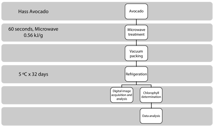
Figure 6.1 Diagram of the methodology.
- Vacuum packing. Then, the dip is vacuumed packed.
- Refrigeration. Finally, the dip is refrigerated at 5°C for 32 days.
- Analysis. A sample is obtained for analysis every 4 days. Specifically, digital image acquisition and chlorophyll determination are performed. Details regarding the chlorophyll determination can be found in the study of Ramirez-Gomez [10].
6.3 Image Acquisition
Matlab 2015, image acquisition toolbox and image processing toolbox, was used for image acquisition and processing.
Images are acquired using a standard USB camera, which returns images in the YUY2 color space. These images were transformed to red–green–blue (RGB) space.
The experimental setup is shown in Figure 6.2. It is important to remark that a designed cylindrical container for placing the avocado dip was made in order to reduce noise on images coming from lighting environment.
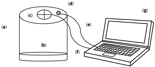
Figure 6.2 Diagram of the image acquisition setup with connection to a laptop. (a) The body of the cylindrical container is made of a nonreflecting white plastic. (b) The base where the avocado dip is placed. (c) The hollow where the cylinder USB camera is screwed. (d) The hollow where a USB cable comes out to power the illumination leds. (e) The cable for powering the leds that connects to a USB port from the laptop. (f) The cable that powers the USB camera and gets the images to the laptop (g) using a USB port.
6.4 Image Processing
As mentioned earlier, color is highly important to determine the freshness of the avocado dip. The image processing to analyze the avocado dip color was performed as follows:
- First, for each image, the average color (ra, ga, ba) is computed in RGB color space by components:
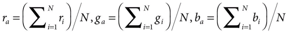
where (ri, gi, bi) is ith pixel in the image, and N is the total number of pixels in the image.
- Second, to obtain invariance of color to illumination changes, the average color in the RGB space is transformed to the L*a*b* color space.
- Finally, scatter plot diagrams and bivariate frequency histograms were generated to study the color distribution of each image in a*–b* space (see Figures 6.5–6.8).
6.5 Experimental Design
Two experimental designs were performed to analyze color changes on avocado dip under different conditions.
6.5.1 First Experimental Design
To analyze the color on the avocado dip, image colors of avocado dip samples were computed in RGB color space. The timeline analysis of the samples was of 48 hours. A color analysis was performed at 0, 4, 24, and 48 hours. These samples were processed using two treatments:
- Sample A. The avocado-dip samples did not go under microwave treatment and vacuum packing.
- Sample B. Avocado-dip samples went under microwave treatment and vacuum packing.
6.5.2 Second Experimental Design
To analyze the evolution of avocado dip in a longer period, a timeline analysis of 32 days was used. In this experimental design, image colors of avocado dip samples were transformed from the RGB space to the L*a*b* space, so that the color evolution can be analyzed with independence of illumination. The (a*, b*) components keep the color without influence from the luminance, L* component. These samples were processed using two treatments:
- Sample A. Avocado dip packed in vacuum and kept in refrigeration for 32 days.
- Sample B. Avocado dip packed in vacuum and kept in refrigeration for 32 days. Additionally, microwaves were applied with 0.56 kJ/g.
6.6 Results and Discussion
6.6.1 First Experimental Design (RGB Color Space)
The results that follow are for avocado dip without refrigeration and without vacuum packing.
Figures 6.3 and 6.4 show the avocado dips of sample A (i.e., avocado dip without microwave treatment) and sample B (i.e., avocado dip was subjected to microwave treatment), respectively. Regarding sample A, it can be seen that the avocado dip color only stayed green at the 0 hour. It changed to brown color after 4 hours from its treatment. On the other hand, it can be noticed that the avocado dip color of sample B remained green after 24 hours from its treatment. Consequently, microwave treatment (sample B) kept the green avocado dip color for 24 hours more than treatment without microwaves (sample A).
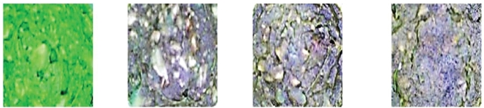
Figure 6.3 Avocado dip samples without microwave treatment taken at 0, 4, 24, and 48 hours.
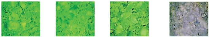
Figure 6.4 Avocado dip samples with microwave treatment taken at 0, 4, 24, and 48 hours.
6.6.2 Second Experimental Design (L*a*b* Color Space)
Figure 6.5 shows the color evolution in a*–b* space without microwave treatment, whereas Figure 6.6 displays the results with microwave treatment. The results show that using the proposed microwave energy, 0.56 kJ/g, avocado dip is preserved greener than the control sample for all the times tested, with no refrigeration, and with refrigeration, 5°C, under vacuum packing.
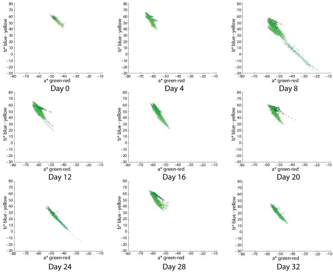
Figure 6.5 Distribution color plots in a*–b* space for each image of avocado dip. The horizontal axis of each plot is the a* dimension, which varies from green to red. The vertical axis of each plot corresponds to b* dimension, which varies blue to yellow. The color of each plotted pixel is located in coordinates (a*, b*), and for graphical purposes the displayed color is the corresponding (r, g, b) value. These plots correspond to images from avocado dip with refrigeration at 5°C, vacuum packing, and without microwave treatment. The images are displayed from left to right from day 0 to day 32 with an interval of 4 days.
Moreover, it can be seen that color in the a*–b* space of the sample B (subjected to microwave, Figure 6.6) is almost always more to the left and above than the sample A (control sample, Figure 6.5). This means that, almost always, its color is greener to yellower, more to the left in the a* dimension (green–red), and more up in the b* dimension (blue–yellow). This reflects the actual color of avocado dip that has a mixture of green–yellow coloration.
Figures 6.7 and 6.8 show an alternative display of color distribution for each image analyzed in a*–b* space. These plots show the joint probability distribution P(a*,b*) of random variables a* and b*. In this case, P(a*,b*) is represented by an unnormalized bivariate histogram. In each plot, the horizontal plane corresponds to the Cartesian product of the intervals, where each random variable, a* and b* vary. Random variable a* varies in the range [−100, 100], corresponding to the variation from color green to color red. Whereas random variable b* varies in the range [−100, 100], corresponding to the variation from color blue to color yellow. The vertical axis represents the frequency in the bivariate histogram. The height/value of each histogram bar at coordinates (a* = ax, b* = by) is equal to the number of pixels that simultaneously attain the color value (a* = ax, b* = by). The color of the bars in the bivariate histogram is represented using a “heat” color map which varies in the colors: blue, light blue, green, orange, and yellow, in correspondence from lower to higher frequencies. For instance, if a few pixels obtain a pair of values (a* = ax, b* = by), in the histogram, for that point, it will be represented with a short blue bar. In contrast, if many pixels obtain a particular combination of pair of values, the histogram on that position will display a large bar which has painted all the mentioned colors in the heat map, and in the highest part of the bar, it will have a yellow color.
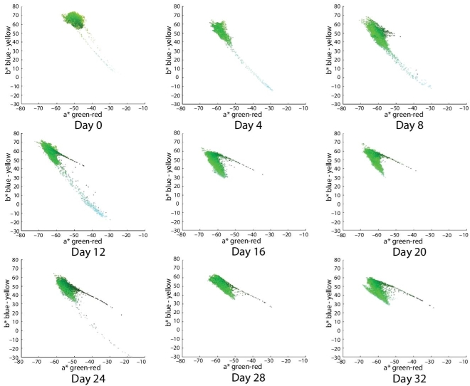
Figure 6.6 Distribution color plots in a*–b* space for each image of avocado dip. The horizontal axis of each plot is the a* dimension, which varies from green to red. The vertical axis of each plot corresponds to the b* dimension, which varies from blue to yellow. The color of each plotted pixel is located in the coordinates (a*, b*), and for graphical purposes, the displayed color is the corresponding (r, g, b) value. These plots correspond to images from avocado dip with refrigeration at 5°C, vacuum packing and with microwave treatment with 0.56 kJ/g. The images are displayed from left to right from day 0 to day 32 in increments of 4 days.
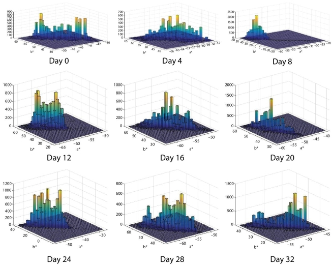
Figure 6.7 Bivariate frequency histogram for a*–b* space for each image of avocado dip. The horizontal plan is formed by a* and b* axes. The vertical axis is the frequency for each (a*, b*) value. The corresponding images of avocado are without microwave treatment.
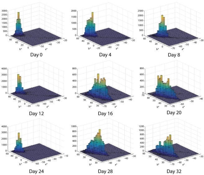
Figure 6.8 Bivariate frequency histogram for a*–b* space for each image of avocado dip. The horizontal plan is formed by a* and b* axes. The vertical axis is the frequency for each (a*, b*) value. The corresponding images of avocado are with microwave treatment.
Figure 6.7 displays the evolution of the bivariate frequency histogram in the a*–b* color space from day 0 to day 32 of the corresponding images for the control sample of avocado dip without microwave treatment.
Figure 6.8 displays also the evolution of the bivariate frequency histogram in the a*–b* color space for the same period of time, but in this case, the sample of the avocado dip received microwave treatment with 0.56 kJ/g.
Additionally, it is important to remark that the designed cylindrical container is useful to have a controlled illumination setting. Moreover, because of the use of computer vision monitoring in the a*–b* space, color invariance to illumination is preserved in a practical way using a standard USB camera. This experimental setting could be of value for laboratories studying the preservation of color for avocado dip under different treatments and for other food science experiments that need to monitor color through time.
6.7 Conclusion
This study presented an experimental setup for analyzing the color of avocado dip through time subjected to laboratory conditions. The analysis was based on color transformations using image processing/computer vision. Images were taken with a standard USB camera and transformed to L*a*b* space because the a*b* components have color invariance to illumination. Avocado-dip samples were analyzed under two experimental designs using different treatments: i) avocado-dip samples with microwave versus avocado-dip samples without microwave; and ii) avocado-dip samples packed in vacuum and kept in refrigeration for 32 days versus avocado-dip samples packed in vacuum, kept in refrigeration for 32 days, and with microwaves applied with 0.56 kJ/g. These treatments were analyzed in order to determine which ones maintain the color longer through time. Sample images were taken every 4 days during the timeline of the experiment. This study showed that avocado dip subjected to microwave energy of 0.56 kJ/g, with vacuum packing, and refrigeration at 5 °C, in an interval time of 32 days, preserved the green-yellow color tones longer than a reference sample without microwave treatment.
References
- 1. Zhang, B., Gu, B., Tian, G., Zhou, J., Huang, J., Xiong, Y., Challenges and solutions of optical-based nondestructive quality inspection for robotic fruit and vegetable grading systems: A technical review. Trends Food Sci. Technol., 81, 213, 2018.
- 2. Moreda, G.P., Muñoz, M.A., Ruiz-Altisent, M., Perdigones, A., Shape determination of horticultural produce using two-dimensional computer vision—A review. J. Food Eng., 108, 245, 2012.
- 3. Zhang, Y., Wanga, S., Ji, G., Phillips, P., Fruit classification using computer vision and feedforward neural network. J. Food Eng., 143, 167, 2014.
- 4. Liu, Y., Pu, H., Sun, D., Hyperspectral imaging technique for evaluating food quality and safety during various processes: A review of recent applications. Trends Food Sci. Technol., 69, 25, 2017.
- 5. Mery, D. and Pedreschi, F., Segmentation of colour food images using a robust algorithm. J. Food Eng., 66, 353, 2005.
- 6. Steinbrenera, J., Poschb, K., Leitner, R., Hyperspectral fruit and vegetable classification using convolutional neural networks. Comput. Electron. Agric., 162, 364, 2019.
- 7. Calvo, H., Moreno-Armendáriz, M.A., Godoy-Calderón, S., A practical framework for automatic food products classification using computer vision and inductive characterization. Neurocomputing, 175, 911, 2016.
- 8. Quevedo, R., Ronceros, B., Garcia, K., Lopéz, P., Pedreschi, F., Enzymatic browning in sliced and pureed avocado: A fractal kinetic study. J. Food Eng., 105, 210, 2011.
- 9. Zhou, L., Tey, C.Y., Bingol, G., Bi, J., Effect of microwave treatment on enzyme inactivation and quality change of defatted avocado puree during storage. Innov. Food Sci. Emerg. Technol., 37, 61, 2016.
- 10. Ramirez-Gomez, E.K., Digital image analysis of avocado dip treated with microwaves. Master thesis in Food Science, University of Veracruz, Mexico, 2019, (in Spanish).
Note
- * Corresponding author: [email protected]