
CHAPTER 8
Valuing Data with Statistical Analysis and Enabling Meaningful Access
“There are thousands of ways to mess up or damage a software project, and only a few ways to do them well.”
—Capers Jones
Applied Software Measurement: Global Analysis of Productivity and Quality
A business organization is not set up to be egalitarian. Certainly, when it comes to social interactions in the workplace, we should always show respect and be courteous to everyone. But organizationally, distinct roles and areas of responsibility require that boundaries be set. Regarding data access, organizational boundaries dictate appropriate permissions and privileges for each employee, determining what can be known and what can be acted on.
This chapter introduces approaches for accessing data determined by your role and responsibility. This includes data that has been valued and intentionally democratized or data that, by design, is not intended to be used as a democratized asset. Performing analytics and artificial intelligence (AI) drives the need for accessing data that is in direct support of the organizational demands for prediction, automation, and optimization.
Deriving Value: Managing Data as an Asset
While data, information, knowledge, and wisdom (DIKW) (discussed in Chapter 7, “Maximizing the Use of Your Data: Being Value Driven”) addresses the formation of a value chain, each point in each chain should be measurable so as to demonstrate value. If the data is to be regarded or treated as an asset, you'll want to apply some type of metric to the asset. Each point in the value chain is an asset in its own right. Return on investment (ROI) is often a default measure of value for organizations.
The purpose of calculating an ROI is to measure, per period, the rates of return on money that has been invested or spent. Using an ROI in casual business conversation is often a means to justify a qualitative benefit over a quantified measure. Calculation of an ROI can be lax, reflecting a sentiment that the ROI expresses a generalization rather than a definitive measure.
For example, suppose $1,000 was invested in some machine learning algorithms. One year later, the algorithms had generated $1,200 in new client sales. To calculate the ROI, the profits ($1,200 – $1,000 = $200) would be divided by the investment cost ($1,000), for an ROI of 20 percent, or $200/$1,000.
Alternatively, $2,000 could have been invested in monitoring and remediating bias in AI models. Three years later, monitoring and remediation helped to generate $2,800 in additional client sales. The ROI on the monitoring and remediation software would be 40 percent, or ($2800 – $2000)/$2,000.
While the second investment yields a higher percentage, when averaged on a per-year basis, the return is 13.3 percent (40 percent/3 years). This would make the first investment more valuable. ROI is used in this type of lax manner when time frames and other indirect costs are ignored.
Another type of measurement is return on assets (ROA). ROA is a metric that can be used to provide an indication as to how efficiently assets are helping to generate earnings. ROA is calculated by dividing an organization's annual earnings by its total assets. As with an ROI, an ROA is presented as a percentage.
In the era of advanced analytics, organizations will want to demonstrate tangible benefits from using data to drive efficiencies through predicting outcomes, providing automation, furthering the optimization of resources, increasing earnings, or expanding presence or market share. Stating the derived value from data should be formalized in a measurement. A return on data assets (RDA) is one such measure.
RDA can be used as a measure for how efficiently an organization is able to generate gains from its data corpus or inventory of data. Because data is inert, data cannot derive its own value. Data cannot be associated with value generation without a deliberate means to provide insight that can be acted upon (value) for the organization.
The term for information within the data topology that is not accessed, or for information that has been rendered inaccessible, is dark data. Dark data is a cost to an organization and yields no value. Additionally, not all data is created equal. This means that certain preserved facts contribute more heavily toward an outcome than other preserved facts. For instance, the date of a customer's last placed order is likely to yield more value to an organization than the middle initial of a customer's name.
Calculating the value of a data asset can be complicated and potentially made more complex by the fact that not all data is created equal, but also because the value of data can change along its value chain. Exposing a formal data value chain can be a good starting point to establish asset values for data (as well as the data's accompanying metadata).
Along the data value chain, data is part of a lifecycle, and each point in the lifecycle represents a tangible resource for the organization. Assessing the data's value is one thing, but knowing how to grow that value can be another organizational challenge altogether. While data has value, data is also a cost and accrues ongoing costs.
The often-used analogy between data and crude oil illustrates how both materials can be used for a diversity of applications as the respective materials are refined and gain in value over the original value of the base raw product. The comparison also brings to the forefront that, like oil, data needs to be considered a tangible asset and be measured as such.
To create value, data typically goes through many steps, from ingestion to integration and from correlation to consumption. The aspect of consumption is where the analogy between data and oil falters as data is an asset that is not depleted upon consumption. Data is an asset that is not depleted upon consumption. Data can be eternal, and while an organization may be able to control certain aspects of the data's longevity, digital derivatives can persist without incurring generational loss outside the auspices and control of the organization.
As an asset, data is fully reusable versus being depletable or renewable. However, over time, data can be subject to a type of decay, which means that given a current context, the values are no longer representative. In all cases, it's the reusability of data as an asset that enables data to participate in a value chain. Understanding the value chain is crucial to building an information architecture that provides an organization with the capability to continually solve business problems with agility, scalability, and AI. As shown in Figure 8-1, smarter data science incrementally adds to the value of data, and every step in the data value chain is vital. While the quality of data does not have to be pristine, a lack of quality can place a negative impact on the value or even negate all value.

Figure 8-1: Data value chain
As a raw material, an intriguing aspect of data is that value can be derived from another organization's data (raw material) and, in some cases, without the need to purchase usage rights or be associated with the normal costs that are attributed to internal data generation.
A use of a data topology can help with providing a general map (vis-à-vis the zone map) for the value chain to overlay. As just explained, not all data zones would need to be organizationally internal data assets. A data zone can, for example, cover external data that is virtualized by the organization. Here, the use of virtualization ensures the external data remains in place and is not formally copied or replicated into another data zone.
The value chain implies that value is further increased by harvesting and processing data that can be repurposed. As such, derivative data products from the raw material are likely to be materialized, and those materialized assets are likely to be incorporated into a data zone that is internal to the organization.
All data sources, internal or external, need to be discoverable, located, and evaluated for cost, coverage, and quality. The ingest pipeline, or data flow, is fundamental to enabling reliable operation throughout the entire data topology, especially as the data flows from one data zone to another. There are diverse file formats and network connections to consider, as well as considerations around frequency and volume.
Following ingestion, the data can be refined. Refinement can condition the data and make it generally usable for the organization. Later, the data can also be transformed into a format that facilitates reuse, or the data can be curated in a manner that provides efficiency through personalization to individuals or teams across the organization.
Distributed storage provides many options for persisting data over the data topology, along with the choice of format or database technology in a leaf zone. The choice of format or technology is often influenced by where in the value chain the data is likely to reside and be consumed. For example, certain formats and technologies are chosen for operational uses versus those that are made for analytics and AI.
Increasing the value in data can often be achieved by combining a variety of data sources together to search for new or previously obscured facts or insights. Integration is a nontrivial but valuable step in the value chain and enables correlation processes to occur. Analytics is dependent on every other step in the value chain.
Data scientists often spend more time in the earlier stages of the value chain because the data is not readied for their activities. The results of advanced analytics and the data that is exposed to the organization's users represent a final point-in-time step in deriving interim value from data. The value does not have to dissipate as the data itself has not been depleted.
Each insight can be evaluated and acted upon. The outcomes that are a result of the action also produce data points that can be fed back into the chain to further improve the value of the data asset.
A decision not to act is also a type of action that can be recorded for feedback. The feedback for nonaction can be used to understand why an action was not taken. The data point could be useful for future understanding and optimization.
As organizations grow their data estates and add to their AI capabilities, evaluating the asset value must be performed so as to ensure an organization can accelerate the means to increase the value of data. Developing a standard RDA metric could prove a useful measure.
The data valuation chain can help illuminate how raw data begets many intermediate forms as it is collected, processed, integrated, correlated, and transformed with context to produce actionable insights, which can lead to an action with a discernible and measurable outcome.
An Inexact Science
Valuing the data asset may be an inexact science due to a multitude of reasons. The data's value can increase or decrease as it moves through the data valuation chain. For example, knowing a customer's home address can have a certain value. However, should the customer no longer reside at that home address, the data may have less value if the current home address remains unknown. If both the old address and the current address are known, additional value can be derived through a better understanding of the longitudinal aspects of the customer.
In this regard, data is measured on a value-based system with regard to the potential value on business action that can be taken. As data progresses through the chain, the value increases or decreases in relation to the ability to act and the end-product value. Data's valuation can depend on where in the chain the data actually lies. Separating the intermediate value of a data asset from the overall value of a completed chain can vary from one chain to the next. Correlating multiple datasets can be worth much more than the linear sum of their combined individual values.
A machine learning or statistical model can exponentially increase the value of a data source, but valuing such analysis must also be predicated on the type of action and the expected outcome.
The valuation of the chain must be completed to aid in realizing the value from the data. In economics, goods can be described as being rivalrous because the consumption of a good can prevent others from consuming the same good. As data is not depleted, the data itself is nonrivalrous.
The initial costs of manufacturing data as a raw material can be expensive, but the marginal costs can decline as the data is refined and flows across the data topology. Deriving value from data can be risky when the value of any resulting business action and outcome is not definite. Quantifying that risk for the data's value can also be difficult.
The same raw data can be a common origination point for multiple value chains. As with the analogy to crude oil, the oil goes through a value chain with the intent of producing a viable product. However, crude oil has a relatively small number of possible end products whose market values are well defined and that are driven by the demand and supply in the global market.
Raw data has the potential to have an indefinite number of possible end-product uses. Each end-product for data can depend on the user and intention and purpose for which the data can be applied, all of which are subject to change over time and possibly frequently.
A retailer may decide to use aggregated GPS information to ascertain which location to use for a store expansion initiative but could subsequently use the same GPS information to determine efficiencies for offering in-home delivery to customers. This can make it difficult to value data in monetization terms through income-based methods. The number of possible uses of data—and, therefore, the potential income associated with the data—can change drastically.
Ultimately, the valuation chain could be completed only to result in yielding no value at all. In economics, goods are viewed as transparent because the buyer typically knows what they are getting before they agree to purchase a good. Data and other information goods can be deemed experience goods. With experience goods, value may not be fully determined until after the goods have been used.
Many different data chains can be established from the same original raw data. As previously noted, persisted data is not a resource that is depleted, and in addition, the data is nonsubtractable. Nonsubtractable means that the use of data does not detract from being applied to other uses. You could use the same data source for multiple forms of analytics and decisions by many different users. So, the value of data may prove highly variable across multiple uses.
While regulations such as the General Data Protection Regulation (GDPR) may limit or even prevent data access for subsequent business purposes, many data assets can continue to be disseminated for additional decision-making.
Different valuation chains might require different levels of data quality. Data quality is multidimensional and can be measured using different means such as accuracy, completeness, breadth, latency, granularity, etc. Different types of analytics may require different levels of quality for each dimension. Data that is regarded as being high-quality data for one use may be regarded as being low-quality data for another use. For example, stock exchange data that has been cleansed and has had its outliers removed may be extremely valuable to long-term financial modelers but inappropriate for data scientists working in the area of fraud detection.
Raw data from completely different sources could provide the same insight and result in the same business actions. While data fuels key business processes and decisions, where the actual data came from is often less important than the actual insight provided. GPS data that is aggregated by telephone providers could provide information on population density that can guide decisions about where to locate a new store, but satellite photographs could potentially provide comparable information.
The derivable value from a data source depends not only on its potential end use but also on whether a substitute data source can be made available. The alternative data source may have differing cost factors as well.
The purpose of providing analytics to an organization is to provide value to the business by serving the organizational analytical delegates. From an analytical user perspective, the following factors are important to understand or to discover:
- The type of content that is accessible
- The level of data quality regarding the accessible data
- The profile of the data that is accessible
- The business metadata, technical metadata, and operational metadata associated with accessible data
- The means by which self-service is available to enrich, cleanse, enhance, and aggregate the accessible data
- The means by which to annotate and tag the accessible data
In this context, accessible data implies the range of data a single user has permission to consume. What data is accessible can vary by user, and being able to understand or discover each of the preceding items is dependent on the information architecture along with the provisioning of unified data governance and the appropriate security rules.
Accessibility to Data: Not All Users Are Equal
In previous chapters, we noted that not all data is created equal; certain data will yield significantly more benefit to the organization than other pieces of data. Aspects of inequality can also apply to other organizational assets, including employees. Because an organization designates that each employee is given a discrete set of roles and responsibilities, we can infer that the data privileges afforded to each employee might also vary from one employee to the next; not all employees are created equal.
By virtue of each unique role and responsibility, there can be a shift in what information an employee is entitled to view or manipulate and what information they are not entitled to view or manipulate. Curated data stores, as discussed in Chapter 7, can be a means to ensure an employee not only receives the data they are entitled to use but also receives it in a format that promotes work efficiencies.
Furthermore, what data is made accessible to one user and what data is made available to another user can impact derived insights. While it is easy to understand that through implemented security measures a single user should see only what they are entitled to see, how business results can be impacted can be a little bit more subtle.
Suppose a data zone has three datasets: Dataset A, Dataset B, and Dataset C. If one user has access to all three datasets and another user has access to only two of the datasets, different results (or insights) can be gained or lost depending on the privilege to access. If both users need to correlate data, a scenario could play out in this manner:
- User 1 has permission to access Dataset A, Dataset B, and Dataset C. In Dataset A is a record for Eminem. Dataset B has a record for Marshall Mathers, and Dataset C has a record for Slim Shady. When correlating the three datasets, Dataset C has the requisite data points that enable combining all three persons together as a single individual. The result is a single person record with three name aliases.
- If User 2 does not have permission to access Dataset C, the ability to correlate some of the data between Dataset A and Dataset B is lost. The result is two distinct person records with no known aliases. There is now a true sense of irony to the question, “Will the real Slim Shady please stand up?”
While accessibility to data is always in accordance with security and permission, accessibility has another dimension in terms of whether the information is accessed on your behalf or whether the data can be self-accessed.
Providing Self-Service to Data
Self-accessed or self-service implies that either a technical professional or a nontechnical business user can access and analyze data without involving others from an IT department. Self-service means that all users can—regardless of their job responsibilities—access data without the need for formal assistance from an IT department. Data scientists and citizen data scientists alike are trusted with the tools to achieve their mission within the organization.
In a self-service model, users gain access to the metadata and data profiles to aid them in understanding each attribute or feature in a dataset. Captured metadata should provide enough information for users to establish new data formats from existing data formats, using a combination of enrichment and analytics.
The data catalog is a foundational tool for users to discover data or to discover machine learning models. Users should also be able to look for any kind of feature. Examples include searching across a timeframe such as February 1 to February 28 and searching on a subject area such as marketing or finance. Users should also be able to locate datasets based on included features, such as finding datasets than contain features for a 30-year bond or a feature that contains a percentage.
Discovery should also include the means to uncover data based on classification, quality levels, the data's lineage, the model's provenance, which assets have been enriched, or which are in need of enrichment. Cognitive-driven discovery would also enable the recommendation of assets to further aid the users in driving insights.
The accumulation of business metadata, technical metadata, and operational metadata is critical for maintaining a data catalog. Users may also want to see the historical activity for all of the ingested data. If a user is looking at streamed data, a search might be conducted for days when no data came into an organization. The intent of the user would be to ensure that those days are not included in the representative datasets for campaign analytics. Overall, access to data lineage, the ability to perform quality checks, and view ingestion history can yield a good sense of the data, so users can begin their analytic tasks.
A catalog is essential for maximizing the accessible data in the data topology. The data topology represents an enterprise-grade approach to data management as the data topology is not necessarily constrained to serving just one aspect of the organization. In support of self-service, the catalog also needs to provide an enterprise-grade view. As organizational users collaborate, a catalog can leverage credentials so that collaboration can be meaningful by applying data protection policies to protect sensitive data through either redaction or the anonymization of data and to ensure controlled access.
Access: The Importance of Adding Controls
When providing various users with the tools they need, security over the data remains a critical capability. Setting and consistently enforcing the security policies is essential for the long-term viability of the data supported through the information architecture. Security features should not be restricted to the consumption data but also include the data zones that might be exclusively used for data preparation and data enrichment.
Because data scientists may need more flexibility, with less formal governance, an exploration and discovery data zone is often established for them. In general, data scientists must be practiced in the management of sensitive data. A data catalog should be able to indicate data that is sensitive, but don't assume that the catalog is always used. Data must always remain tightly controlled.
With security policies in place, users should have access only to the datasets assigned to their security profile or level of privilege. However, because the data afforded a data scientist may be untethered or unmonitored, the data may be susceptible to leakage.
Data leakage is the distribution of private or sensitive data to someone who is not authorized to view the data. The delivery of leaked data can be unintentional. Data from the discovery and exploration data zone can be vulnerable to leakage, especially if a data scientist is given open access to that data.
Data leakage can be exacerbated by the fact that data might not follow the data flows indicated by the data topology for both inbound and outbound data. An information architecture must ensure that data flows do not go unregulated and unmonitored.
The adverse consequences of a data leakage incident can be classified as a direct loss or an indirect loss. Direct losses are generally tangible and can be easy to measure or estimate quantitatively. Indirect losses are associative and may be more difficult to access in terms of cost, place, and time. A direct loss can include violations of regulations resulting in fines to the organization, settlements or customer compensation fees, litigation involving lawsuits, loss of future sales, costs of investigation, and remedial or restoration fees. Indirect losses can include reduced share prices for publicly traded companies as a result of negative publicity, damage to an organization's goodwill and reputation, customer abandonment, and the potential exposure of intellectual property.
Access controls also enable collaboration. For example, a user might find a dataset that is important to a project and be able to interactively share findings with other colleagues, while in turn those colleagues provide various enrichments.
While many controls are enacted top-down through security and data governance, certain usage can be garnered in a bottom-up approach as well.
Ranking Datasets Using a Bottom-Up Approach for Data Governance
The bottom-up approach to data governance enables the ability to rank the usefulness of datasets by asking users to rate the value of a given dataset. The ranking can greatly assist cognitive-driven discovery capabilities that are used to further recommend assets.
An ability to rate a dataset leverages crowdsourcing techniques from an internal group of users. Internal-based crowdsourcing can help to establish a preferred source to access data rather than being directed to the source via top-down governance.
Tools are required to help create new data models from existing datasets. An example is taking a customer dataset and a transaction dataset to create a customer dataset based on predictions for total lifetime customer value (LCV). Performing these types of enrichments and transformations is important in providing a holistic framework for delivering advanced analytics, especially by the citizen data scientist, regardless of their associated industry.
How Various Industries Use Data and AI
In Chapter 7, we discussed how design choices can be influenced based on your understanding of the value of data and the value chain for serving different points of the business, e.g., order intake versus order fulfilment versus order completion, etc. Across different industries, within an industry, and across the different lines of business, products, services, and customers, the orientation as to what types of models can provide significant business impact can vary.
As a common foundation, an information architecture can prove to be an enabler for providing value for many different vertical industries that seek to benefit from AI. Here are some examples:
- Healthcare providers can maintain millions of records for millions of patients, encompassing structured, semistructured, and unstructured data from electronic medical records, radiology images, and doctors' notes. Leveraging advanced analytics can be performed to enable payments, mitigate instances of fraud, predict readmissions, and help frame future coverage. Raw data helps preserve the data in an untampered state, and lifecycle management practices enable data offloading after a prescribed period of time.
- Financial service organizations must comply with various fiscal regulations depending on the country in which they operate. The data zones can aid reconciliation, settlement, and regulatory reporting.
- Retail banking also has important use cases where advanced analytics can help reduce first-party fraud, anti-money laundering (AML), and other financial crimes.
- Retailers can help improve the customer experience by positioning the correct products to up-sell and cross-sell. Advanced analytics can be used to provide timely offers and incentives.
- Governments can help improve citizen experiences by ensuring that citizens receive the services they need when they need them.
- Telephone companies can seek to reduce churn and to also understand the demographic concentration of certain areas by monitoring call times and call durations. Cellular companies can detect cell tower issues by associating dropped calls.
- Manufacturers are always sensitive to increasing efficiency. By using designated data zones to serve as a gateway between connected devices and the Internet of Things (IoT), AI can help to provide predictive analytics to connect factories and optimize the supply chain.
In each of the industry use cases, there are likely to be outliers and exceptions. Statistics can provide the requisite insight to fine-tune AI models or, with the establishment of a series of ensemble models, to create a desirable outcome.
Benefiting from Statistics
As data will be accessed and used across the value chain and whether provisioned by IT or self-served, statistically interpreting the data can be beneficial. Not only will statistics help you with how to rank a data asset, you'll also find ways that will provide greater insight into placing a value on the data too. And, depending on which industry you're working in, you may be oriented to specific statistical methods that you'll want to apply.
In statistics, a normality test is often used to determine whether the data reflects what could be considered a normal distribution. There are many statistical functions that are used in conjunction with AI that rely on the data's distribution to be regarded as being normal or nearly normal. Statistically, there are two numerical measures of shape that can be used to test for normality in data. These numerical measures are known as skewness and kurtosis.
Skewness represents a measure of symmetry or, more precisely, a measure that can represent the lack of symmetry. A distribution is symmetric if the data point plots look the same to the left and to the right of the center point. A kurtosis is used as a measure to show if the data is heavy-tailed or light-tailed, relative to a normal distribution.
As shown in Figure 8-2, there can be a positive skewness and a negative skewness. A fully symmetrical distribution has a skewness of zero, and the mean, mode, and median will share the same value.
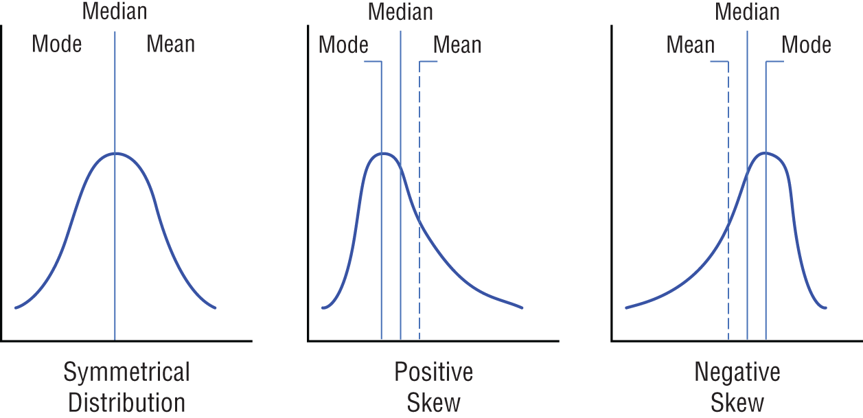
Figure 8-2: Skewness
The mean is the average number that is calculated by summing all of the values divided by the total number of values. So, the mean for the values 1, 10, 100, and 1000 would be 1111/4, which is equal to 277.8.
The mode is the most frequent value that occurs in a set of data. If the values for a given set are 1, 5, 2, 6, 2, 8, 2, and 34, the most frequently occurring value is 2. The number 2 as the most frequently occurring value can be readily seen should the values be sorted in ascending sequence: 1, 2, 2, 2, 5, 6, 8, 34.
In a list of sorted values, the median is the middle number. If our values are 1, 2, 3, 4, 5, 6, and 7, then the middle number is 4.
A positive skewness means that the tail on the right side of the distribution is longer, and the mode is less than both the mean and median. For a negative skewness, the tail of the left side of the distribution is longer than the tail on the right side, and the mean and the median are less than the mode. When calculating the skewness, know the following:
- A result that is between 0 and –0.5 (a negative skewness) means that the data is reasonably symmetrical.
- A result that is between –0.5 and –1.0 (a negative skewness) means that the data is moderately skewed.
- A result that is between –1.0 or higher (a negative skewness) means that the data is highly skewed.
- A result that is between 0 and +0.5 (a positive skewness) means that the data is reasonably symmetrical.
- A result that is between +0.5 and +1.0 (a positive skewness) means that the data is moderately skewed.
- A result that is between +1.0 or higher (a positive skewness) means that the data is highly skewed.
Suppose house prices ranged in value from $100,000 to $1,000,000, with the average house price being $500,000. If the peak of the distribution was to the left of the average value, this would mean that the skewness in the distribution was positive. A positive skewness would indicate that many of the houses were being sold for less than the average value of $500,000.
Alternatively, if the peak of the distributed data was to the right of the average value, that would indicate a negative skewness and would mean that more of the houses were being sold for a price higher than the average value of $500,000.
The other measure regarding the normality of the distribution is kurtosis. With kurtosis, a resulting value describes the tail of the distribution rather than the “peakedness.” A kurtosis is used to describe the extreme values and is a measure of the outliers present within the distribution.
Data with a high kurtosis value is an indicator that the data has heavy tails or excessive outlier values. For AI, a high kurtosis might require a separate model to address the outliers to improve how a particular cohort is handed. A low kurtosis is an indicator that data has light tails or a lack of outliers. Potentially, you'll consider data with a low kurtosis preferable over a high kurtosis.
Figure 8-3 illustrates three types of kurtosis curves: leptokurtic, mesokurtic, and platykurtic.
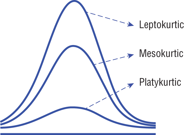
Figure 8-3: Kurtosis
Leptokurtic curves have a kurtosis value that is greater than 3. The leptokurtic distribution is longer with tails that are fatter. Additionally, the leptokurtic peak is higher and sharper than that of the mesokurtic curve, which means the data is heavy-tailed or has an abundance of outliers. Outliers cause the horizontal axis of a visual histogram graph to be stretched, which makes the bulk of the data appear within a narrow vertical range.
Mesokurtic distributions have a kurtosis statistic that is similar to that of the normal distribution and implies that the extreme values of the distribution are similar to that of a normal distribution characteristic. The mesokurtic distribution has a standard normal distribution and a kurtosis value of 3.
Platykurtic distributions are shorter, and their tails are thinner than the normal distribution. The peak is lower and broader than with the mesokurtic distribution. A platykurtic distribution means that data are light-tailed and have a lack of outliers. The lack of outliers in the platykurtic distribution is because the extreme values are less than that of the normal distribution.
Being able to calculate the skewness and kurtosis allows data scientists to create specialized models to handle certain portions of the data rather than through a single generalized model. The skewness or kurtosis calculation allows for specific data points to be identified. Figure 8-4 plots a data population that includes a number of extreme outliers.
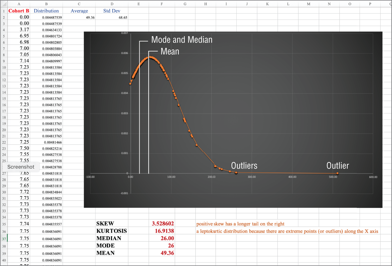
Figure 8-4: Identifying outliers
Understanding skewness and kurtosis means that a data scientist can more readily recognize that an answer to a question can more than likely yield a variety of acceptable answers. In preparing a model, the data scientist is not necessarily expecting one answer, but a range of all different options, and the distribution provides a tendency toward potential answers. This is especially useful when seeking to draw a conclusion about the population of data from a particular sample set.
While exploring various features for a model, data scientists must use statistics to infer values. Should a data scientist have access to a complete dataset, then an exact average known as the true mean can be calculated. If a sample is chosen at random rather than observed, then the expected mean could vary from the true mean. A sampling error is the difference between the sample mean and the true mean.
A standard error refers to the standard deviation of all the means. The sampling error shows how much the values of the mean of a bunch of samples differ from one another.
In Figure 8-4, column B is named “Distribution” and is the normal distribution value of the data in the column named “Cohort B.” The distribution is associated to the shape the data has when represented as a graph. The bell curve that is calculated in the figure is one of the better-known distributions of continuous values. The normal distribution in the bell curve is also known as the Gaussian distribution.
The Python code shown in Figure 8-5 can create an idealized Gaussian distribution.
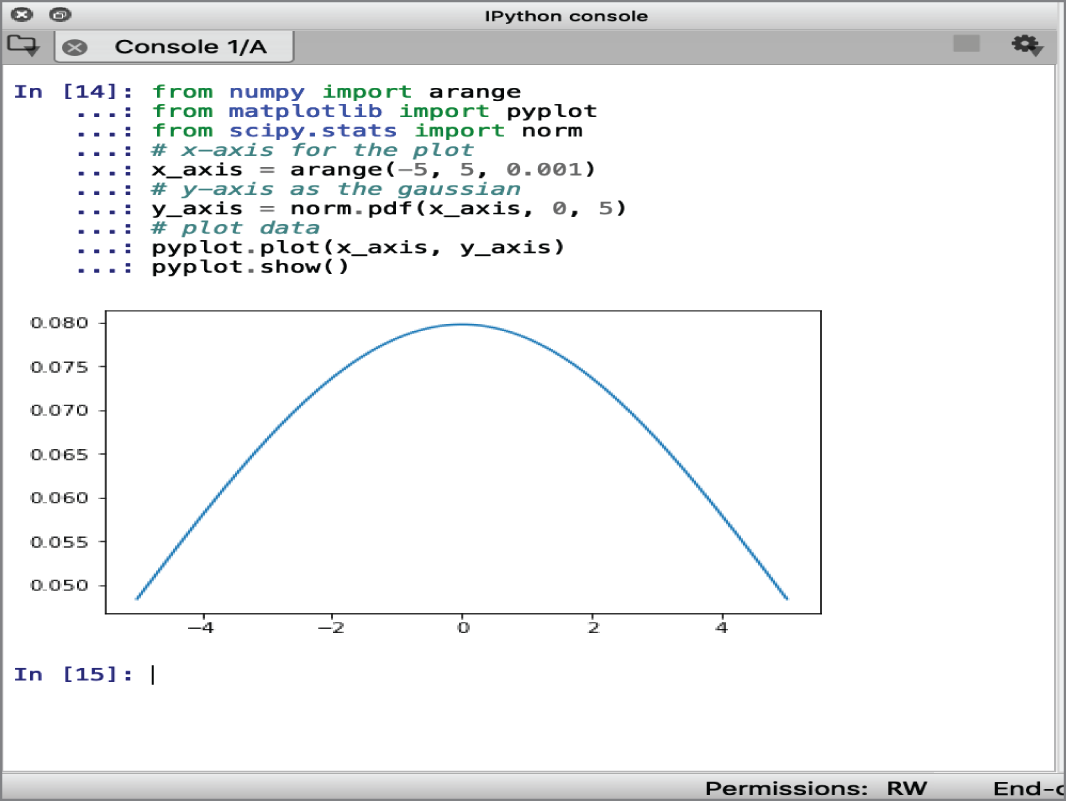
Figure 8-5: Gaussian distribution
In Figure 8-5, the x-axis represents the observations, and the y-axis shows the frequency of each observation. The observations around 0.0 are the most common, and observations around –5.0 and +5.0 are rare.
In statistics, many methods are dedicated to Gaussian type distributions. In many cases, business data that is used in conjunction with machine learning tends to fit well into a Gaussian distribution. But not all data is Gaussian, and non-Gaussian data can be checked by reviewing histogram plots of the data or using statistical tests. For example, too many extreme values in the data population can result in a distribution that is skewed.
Data cleansing can be used to try to remediate or improve the data. Cleansing activities may involve the need to remove all of the outliers. Outliers must be identified as special causes before they are eliminated. Normally distributed data often contains a small percentage of extreme values, and that can be expected to be normal. Not every outlier is caused by an exceptional condition. Extreme values should be removed from the data only if the extreme values are occurring more frequently than expected under normal conditions.
The collected data is referred to as a sample, whereas a population is the name given to all the data that could be collected:
- A data sample is a subset of observations from a group.
- A data population is all of the possible observations from a group.
The distinction between a sample and a population is important because different statistical methods are applied to samples and populations. Machine learning is more typically applied to samples of data. Two examples of data samples encountered in machine learning are as follows:
- The train and test datasets
- The performance scores for a model
When using statistical methods, claims about the population are typically inferred from using observations in a sample. Here are some examples:
- The training sample should be representative of the population of observations so that a useful model can be fitted.
- The test sample should be representative of the population of observations so that an unbiased evaluation of the model skill can be developed.
Because machine learning works with samples and makes claims about a population, there is likely to be some uncertainty. The
randn() NumPy function in Python can be used to generate a sample of random numbers drawn from a Gaussian distribution. The mean and the standard deviation are two key parameters used for defining a Gaussian distribution.
The
randn() function in Python can be used to generate a specified number of random numbers. The scenario shown in Figure 8-6 creates 100,000 random numbers drawn from a Gaussian distribution. The mean and standard deviation are scaled to 50 and 5. To prevent the histogram from appearing too blocky, the option “bins=140” has been added to the plot for the histogram.
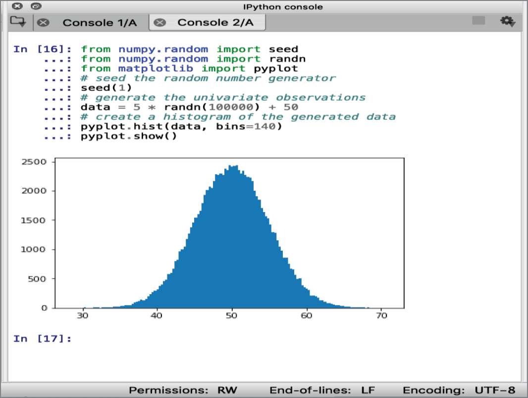
Figure 8-6: Gaussian histogram plot
The nonperfect curve results from the fact that the numbers were randomly chosen and that a degree of noise was introduced into the data sample. Noise is often expected in a data sample.
The central tendency of a distribution refers to the middle value in the distribution, which is the most likely value to occur in the set. In a Gaussian distribution, the central tendency is called the mean and is one of the two main parameters that define a Gaussian distribution. The mean of a sample is calculated as the sum of the observations divided by the total number of observations in the sample. In Python, the mean can be calculated as follows:
The mean calculated from the random data sample in Figure 8-6 is 50.026 and is an estimate of the parameter of the underlying Gaussian distribution. As an estimate, the number is reasonably accurate, as the true mean would be 50.
The mean is influenced by outlier values, and the resulting mean may be misleading. With outliers or a non-Gaussian distribution, an alternative central tendency can be based on the median. The median is calculated by sorting all data and then locating the middle value in the sample. For an odd number of observations, this is quite straightforward. If there are an even number of observations, the median is calculated as the average of the middle two observations. In Python, the median can be calculated as follows:
The median calculated from the random data sample in Figure 8-6 is 50.030. The result is not too dissimilar from the mean because the sample has a Gaussian distribution. If the data had a non-Gaussian distribution, the median may be very different from the mean and could be a better reflection of the central tendency of the underlying population.
The variance in a distribution refers to how much, on average, the observations are varying or differing from the mean value. The variance measures the spread in the distribution. A low variance has values grouped around the mean and exhibits a narrow bell shape. A high variance has values that are spread out from the mean and produce a wide bell shape.
Figure 8-7 shows an idealized Gaussian with low and high variances. The taller plot is the low variance with values grouped around the mean, and the lower plot is the higher variance that has more spread. In Python, the variance can be calculated as follows:
The variance calculated from the random data sample in Figure 8-7 is 24.917. The variance of a sample drawn from a Gaussian distribution is calculated as the average squared difference of each observation from the sample mean.
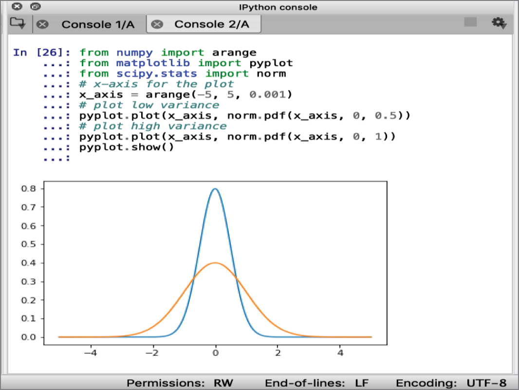
Figure 8-7: Gaussian distribution with low and high variance
When a Gaussian distribution is summarized, the square root of the variance is used. In this case, the square root of 24.917 would be 4.992. This is also called the standard deviation and is very close to the value of 5 that was used in the creation of the test samples shown in Figures 8-6 and 8-7. The standard deviation and the mean are required to specify a Gaussian distribution. In Python, the standard deviation can be calculated as follows:
In applied machine learning, the estimated skill of the model on the output-of-sample data results needs to be reported. The report often reflects the mean performance from a k-fold cross-validation, or some other repeated sampling procedure. When reporting, model skill reflects the summarization of the distribution of skill scores.
In addition to reporting the mean performance of the model, the median and the standard deviation should also be included along with the size of the sample.
Summary
This chapter focused on the importance of and difficulties associated with providing a quantitative value for data. If an organization wants to treat data as an asset, then the asset needs to be given a valuation. The data value chain illustrated that value is not static, and depending on whether the data is in its raw state, refined, or correlated with other data assets, the value can change. Potentially, the value increases as the data moves through the data value chain.
Data is not always fully democratized, and differing security profiles mean that the value different users can extract from the data can also cause complications in the valuation of a data asset.
Data needs to be accessible, and to be accessible, the data must be discoverable. Data assets that are exposed through the use of a catalog also have the opportunity to support the self-service needs of an organization. The ability for datasets to be rated for usefulness can help steer self-service and further improve the benefits of providing a cataloging capability.
As an asset to the organization, data always needs to be protected and secured. The trust afforded to the data scientist can expose weaknesses in a security plan as data can be subject to leakage.
Statistical literacy, with a core facet being anchored to data awareness, helped to showcase how some fundamental statistical knowledge could promote a data scientist's awareness of results from machine learning and deep learning models. The awareness would come from identifying and addressing data that potentially falls outside that of a normal distribution.
In the next chapter, a number of issues that can serve to promote the long-term viability of an information architecture, as well as a deeper dive into data literacy, are explored.