Chapter 8
Cost Approach
8.1 Introduction
The comparison and income approaches to estimating market value are predicated on the availability of market price information. For certain types of land and property, market trading is sparse or non‐existent. If there is no existing market for the tenure rights, then it may be possible to ‘create’ one using an auction or tender process. This approach may be appropriate in the case of large‐scale land acquisitions or the sale of unusual rights such as airwaves for mobile phone networks. If this is not possible, then a cost approach may be appropriate. Two cost approach methods are described in this chapter: the replacement cost method and the residual method.
The replacement cost method is used to value properties that rarely, if ever, trade on the open market and therefore there is little or no evidence of comparable market prices on which to base value estimates. Some properties are very use‐specific: bespoke manufacturing plants such as chemical works and oil refineries; public administration facilities such as prisons, schools and colleges, hospitals, town halls, art galleries and court facilities; and transport infrastructure such as airports and railway buildings. The method is used to value properties for financial reporting, taxation, and expropriation purposes. It is also used to estimate building reinstatement costs for insurance purposes. It is important to note that, when these sorts of properties are offered for sale, perhaps because they are no longer required for their current use, the primary market is likely to be for alternative uses for which a different valuation method may be appropriate.
The residual method is used to value the development potential of land. If a valuer thinks land is not being used to its full potential, it may have development value. Obtaining comparable evidence of development land values can be very difficult; each site is different in terms of size, condition, potential use, permitted density of development, restrictions and so on, adjusting a standard value per hectare almost impossible. The residual method is based on a simple economic concept: the development value of land can be calculated as a surplus or residual remaining after estimated development costs have been deducted from the estimated value of the completed development.
8.2 Replacement cost method
The replacement cost method is used to value property ‘…that is rarely, if ever, sold in the market, except by way of a sale of the business or entity of which it is a part, due to the uniqueness arising from its specialised nature and design, its configuration, size, location or otherwise’ (RICS Global Glossary). So, the value of a specialised property is intrinsically linked to its use and is only appropriate if continued exiting use is envisaged.
The method does not actually calculate a market value. Instead, it calculates a replacement cost for the improvements that have been made to the land, typically in the form of buildings and ancillary man‐made land uses such as car parks, storage facilities and so on. Because of an almost complete lack of comparable market transaction information, the method relies on the economic principle of substitution to regard replacement cost as a proxy for exchange price. In other words, the value is essentially a deprival value of the property to the owner by assuming that the value of the existing property is comparable to the cost of providing a modern replacement that offers an equivalent service potential.
There are two parts to the replacement cost method, a valuation of the land in its existing use and unimproved state and a valuation of the improvements1 to the land. The land is usually valued using the sales comparison method. The improvements are valued by estimating the cost of constructing a new replacement and then applying a depreciation allowance to reflect any deterioration and obsolescence inherent in the existing property.
The three main components of the replacement cost method are considered below: the cost of replacing the building(s) and other site improvements as appropriate, the depreciation of this cost and the valuation of the site.
8.2.1 Replacement cost
The replacement building and site improvements should be functionally equivalent to the subject property. This means that the modern equivalent replacement may not be the same size, layout, design and specification as the actual property. When estimating replacement building costs, the valuer needs to decide what constitutes the building and what constitutes plant and machinery. Sometimes, relatively standard properties have specialised features and adaptations and a valuer may decide that comparable evidence is available for the property and the specialised features can be valued separately using the replacement cost method. Some specialised features may have no market value and could have a negative value if they are regarded as an encumbrance.
The replacement cost will cover all the usual costs associated with the construction of a building, including setup costs (planning fees, site preparation), building costs, professional fees, a contingency allowance, and finance (unless there is an assumption of ‘instant build’) but not developer's profit. If replacement is likely to take a long time, then it may be justifiable to forecast variations in costs.
Professional fees are usually estimated as a percentage of the building cost. Complex schemes or highly specialised buildings may require specialist cost professionals such as quantity surveyors, civil engineers, and structural engineers.
The cost of finance for the construction can be calculated in one of two ways, both of which average the drawdown finance requirement over the estimated length of the construction period. Either calculate compound interest on half of the construction costs at the finance rate for the whole construction period or calculate compound interest on all the construction at the finance rate for the half of the construction period.
If the premises are historic, the extra cost associated with their direct replacement is usually ignored if the service or output could be provided from modern equivalent premises. However, if the historic nature of the premises is intrinsic to the use (a museum for example), then the cost of reproduction would be appropriate. If reproduction is not feasible, the construction of a building with a similarly distinctive design and specification might be appropriate. Of course, some buildings may simply be irreplaceable.
Estimates of construction costs can be obtained from professional cost estimators (quantity surveyors), cost manuals, builders and contractors. The actual cost of constructing the original property may be useful evidence once it has been adjusted for inflation, but with due consideration for any variation that might be due to the existence of a prepared site, the need to reconstruct as quickly as possible, possible changes to planning policy, building regulations and so on.
8.2.2 Depreciation
Because the subject property already exists, and may have done so for some time, the cost of an equivalent new one should be written down or depreciated to reflect any diminution in value. This might be due to age (and estimated remaining economic life2), comparative efficiency, functionality and running costs. The building is valued as it is, taking account of any lack of repair and maintenance, but, looking ahead, an assumption of routine repair and maintenance is acceptable.
Throughout a building's life, its value will tend to depreciate for two principal reasons: deterioration and obsolescence. Deterioration results from wear and tear and is hastened by a lack of maintenance. It is usually measured by reference to the estimated economic life of the asset. It is not easy to generalise about the life of various building types, but prime shop units are much less prone to deterioration than industrial units due to the nature of the use of the building and the proportion of total value attributable to land. Usually, occupiers and owners will want to delay the onset of deterioration as much as possible and this is achieved through good design and construction and active property management. Sound maintenance and management policies help to identify, plan and budget for the onset of deterioration. But inevitably, as the building gets older, maintenance costs increase and the rental value falls because the building is no longer modern and attractive. Consequently, the value of the building declines relative to site value until it becomes economically viable to redevelop the site.
Obsolescence refers to a decline in value resulting from changes that are extraneous to the property. It is a decline in utility not directly related to physical usage or the passage of time. A good‐quality, flexible design can combat obsolescence but, to a certain extent, matters are beyond the control of the property owner or occupier and management and maintenance will have little impact. A building may become obsolete for any number of reasons that rarely work in isolation. Common forms of obsolescence are:
- Functional. The property can no longer be used for its intended purpose, perhaps due to technological changes rendering layout, configuration or internal specification of the property obsolete, and adaptation is not economically viable. Similarly, a property may be adequate in terms of its physical characteristics but is in the wrong location.
- Socio‐economic changes in the optimum use for a site due to market movements may render the existing use obsolete, the building may not depreciate but the development potential of the site appreciates due to changes in the social fabric of the locality or changes in consumer demand, working environment and so on.
- Aesthetic. Image and design requirements are constantly changing and a property that no longer projects the right image may become obsolete.
- Regulatory. This includes changes in planning policy, environmental regulations, health and safety legislation, and lease terms for example.
Whereas physical deterioration may be a continual but gradual process, obsolescence may strike at irregular intervals regardless of age. The responsibility for maintaining the physical condition of a property is usually passed on to the tenant when a commercial property is let on full repairing and insuring (FRI) lease terms, but the risk of obsolescence cannot be managed in this way and is ultimately borne by the owner. The onset of deterioration and obsolescence can be measured by looking at the depreciation in value of the building in relation to modern replacements and by looking at the development value of the land in comparison to its value in its existing state. A sudden switch in the relative magnitudes of development land value and existing use value may occur because of a ‘trigger event’ that presents an opportunity for a more valuable use such as the granting of planning permission. For example, suppose a small industrial estate located on the edge of a town is around 15 years old and the units are looking a little tired. The owner can fill the units with small businesses paying low rents. A by‐pass has recently been constructed around the town and accessibility to the industrial estate is greatly improved. At the same time ‘factory outlet shopping’ has become popular and planning permission to allow an element of retail trade from the industrial units is forthcoming. The owner of the industrial estate anticipates being able to charge higher rents to the factory outlet traders and therefore decides to redevelop the site.
Depreciation can vary according to type of structure and obsolescence may affect different parts of building at different rates. To counter depreciation, there may be a trade‐off between spending more money on the initial design and specification of the building, thus achieving relatively low future costs‐in‐use, or spending less at the start and instead spending relatively more to maintain the premises over its life. The time value of money affects this trade‐off significantly. In quantifying the diminution in value that results from depreciation, the objective is to reflect the way the market would view the asset. When there is a group of buildings to be valued, it is important to consider alternative uses for the premises and their associated lifespans. It is reasonable to assume that routine servicing and repairs are undertaken when estimating lifespan but not significant refurbishments or replacement of components. If refurbishment takes place, then the economic life of the building might be extended. Sometimes, obsolescence can be absolute, other times, partial, perhaps rendering less‐efficient service potential.
8.2.2.1 Estimating depreciation rates
A depreciation rate for physical deterioration is usually estimated by comparing the decrease in value of a building of similar age with the value of a new building. The valuer will estimate a lifespan for the property and its remaining economic life. These will be based on the lower of the property's estimated physical life or economic life, although these are often the same in practice. Physical lifespan assumes the property could be used for any purpose and economic lifespan assumes it is used only for its designed purpose. Both ignore replacement of parts, refurbishment or reconstruction but include routine repairs and maintenance.
A depreciation rate for obsolescence might reflect the cost of upgrading or it might reflect the financial consequences of reduced efficiency compared to a modern equivalent. The modern equivalent replacement may be cheaper to recreate than the actual property, in which case the replacement cost already reflects the most efficient property, so no additional adjustment is necessary. Alternatively, an all‐encompassing depreciation rate may be used for both physical deterioration and obsolescence. If separate rates are used, it is important to avoid double‐counting.
There are various techniques employed in practice to account for depreciation over the estimated lifespan of a property and they work by spreading the reduction in value in a regular pattern over the estimated remaining economic life of the premises. Here are four examples:
- Straight line. By far the most common technique, it applies a percentage deduction based on the proportion of estimated remaining economic life of the premises. In this way, it writes off the value of the improvements over their lifetime to zero or to a residual value. For example, a building purchased for £800 000 with an expected five‐year useful life might be depreciated as follows:
Year Value at start of year Depreciation charge Value at end of year 1 800 000 160 000 640 000 2 640 000 160 000 480 000 3 480 000 160 000 320 000 4 320 000 160 000 160 000 5 160 000 160 000 0 - Reducing balance. A fixed percentage depreciation rate is applied. Using this approach, the value is never completely written off to zero. Taking the building again but this time applying a depreciation rate of 20%:
Year Value at start of year Depreciation rate @ 20% Value at end of year 1 800 000 160 000 640 000 2 640 000 128 000 512 000 3 512 000 102 400 409 600 4 409 600 81 920 327 680 5 327 680 65 536 262 144 - S‐curve. A varying rate of depreciation is devised, usually in the shape of an s‐curve to reflect a low rate in early years, accelerating depreciation in middle years but then tailing off in final years. It is important to base the variation on empirical evidence.
- Sinking fund. A sinking fund may be set up that requires an annual investment to replace the capital value of the building at the end of its estimated economic life.
8.2.3 Land value
When estimating land value, a modern equivalent site is assumed to have the appropriate characteristics to deliver the required service potential at least cost. It may not be the same size or location as the actual site. Indeed, the actual site may not be appropriate if the surroundings have changed. For example, it may be an old prison or a hospital in a city centre location, which is now surrounded by housing. It is also important to note that certain public buildings, such as a school or a health centre, need to be in certain localities, and this constrains site selection.
The land value is based on the size of the plot that is required for the use so, if a school is on a 2.5‐ha site when 1.5 ha is sufficient, it would be valued based on 1.5 ha. The land value is estimated by referring to evidence of transactions of comparable size, tenure and location. If the actual site uses space inefficiently or even inappropriately given changes in technology or production, then modern equivalent sites should be considered. The fundamental principle is an economic one; a hypothetical buyer would purchase the least cost site that is suitable and appropriate for the use. The valuer should also consider whether the actual site location is now one that a modern equivalent would use and whether any vacant land at the actual site is still required for a modern replacement. These considerations can be somewhat subjective as vacant land may be held for expansion, for security or simply may be surplus to requirements.
Because of the specialised nature of the businesses and operations, finding comparable land values is difficult and the valuer may need to broaden the search to include a wider range of alternative site uses. For example, if the use is specialised industrial, then reference to general industrial land prices is usually acceptable. The aim is to select the lowest cost site for an equivalent operation in a relevant location. If the actual site is held on a lease, then the lease terms should be considered when estimating the land value.
The finance cost for the land is estimated by calculating compound interest on the land value over the whole construction period. In other words, the land is assumed to be purchased first and therefore finance is payable for the whole construction period. This finance cost is hypothetical in the replacement cost method because the land is already owned.
Bringing these three components of the replacement cost method together, an example valuation can be presented. A secondary school comprising 3500 square metres (gross) has 12 years of its estimated 50‐year life remaining. Construction costs for a modern equivalent school are £1700 per square metre and the construction period is estimated at 1.5 years. Professional fees are assumed to be 12.5% of building costs. The total site area including playing fields is 11 000 square metres and the land is estimated to be £18 000 per hectare. The local authority, which owns the school, can secure finance for construction and land purchase at a finance rate of 2% per annum.
| Building area (m2) | 3500 | ||
|---|---|---|---|
| Building cost (£/m2) | 1700 | ||
| Cost of modern equivalent building (£) | 5 950 000 | ||
| Fees (% build cost) | 13% | 743 750 | |
| Finance on build cost and fees over half build period @ | 2.00% | 100 157 | |
| Gross replacement cost of building (£) | 6 793 907 | ||
| Depreciation allowance (age/estimated economic life) | 76% | ||
| Net replacement cost of building (£) | 1 630 538 | ||
| Size of site (ha) | 1.10 | ||
| Land value (£/ha) | 18 000 | ||
| Value of land (£) | 19 800 | ||
| Finance on land over build period @ | 2.00% | 597 | |
| Cost of land (£) | 20 397 | ||
| Valuation (before PCs) (£) | 1 650 935 |
The final stage of the valuation is to stand back and look – a final reconciliation to ensure that depreciation has not been double‐counted or ignored and to check whether the characteristics of the property being valued might lead a buyer to bid more than a modern equivalent. When reporting a valuation that is based on the replacement cost method, this must be stated in the report, along with the assumption that the value is subject to the adequate profitability of the company if the property is held in the private sector or subject to the prospect and viability of continued occupation and use if it is a public sector property.
At some point, the property value will fall below the development land value and development becomes viable. This would occur at different times depending on the ratio of land to building components of property value. Figure 8.1 provides an example where there are two sites: a city centre site with a land value of £6m and an out‐of‐town site with a land value of £2m. Building costs and estimated lifespans of the buildings are the same at £5m and 50 years respectively, and the property depreciation rate is 2% in both cases. Because the city centre site has a higher ratio, it has a shorter economic life. Accountants often simplify the process by assuming buildings have standard lifespans, typically 50 years, after which their value is written off, leaving just the land value. In economic terms this would be the point at which land value exceeds building value, signifying redevelopment. Figure 8.1 illustrates this arrangement and shows that now the two properties have the same economic life. This treatment of depreciation is forced by the 50‐years' life‐span assumption.
Figure 8.1 Accounting for depreciation.
8.2.4 Application of the replacement cost method
The valuer may need to agree certain matters with the client as part of the valuation: the potential location of a replacement property, factors that may affect the estimated remaining economic life and details of capital expenditure on maintenance, repairs, improvements, refurbishments, and reconstruction. The valuer is reliant on information provided by the client to a greater extent than for non‐specialised properties, particularly in relation to costs, design features and the performance of the property in relation to its use.
8.2.4.1 Valuation for accounts purposes
If an otherwise conventionally designed property has been specifically adapted (including the installation of plant and machinery), it may be valued subject to a special assumption that the adaptations do not exist and then treating the adaptation costs separately. The valuation should set out which adaptations are included with the property and which have been treated separately.
If the replacement cost value is significantly different from the market value of an alternative use for which planning permission is likely to be forthcoming, both should be reported in the accounts, but the latter need not take account of the costs associated with business closure or relocation. If appropriate, the valuer should report that the value of the premises would have a substantially lower value if the business ceased, but there is no requirement to report a figure.
The initial cost of the property, when first entered into the accounts, can include the purchase costs (such as legal costs and taxes) as well as the purchase price. On subsequent valuations, the reported amount should include purchase or sale costs but these can be stated separately.
8.2.4.2 Valuation for insurance purposes
These are also known as reinstatement valuations and are undertaken on behalf of lenders, normally in conjunction with a market valuation but are also undertaken for insurers and insurance brokers, property owners and occupiers. A reinstatement valuation provides for a similar property as at the date of the valuation or at the commencement of insurance policy cover and should be carried out at least every three years. In the case of insurance valuations, the site is assumed to continue in existence despite whatever disaster may have affected the buildings. Consequently, it does not include a valuation of the land. Furthermore, if the insurance policy provides for a replacement new property (a ‘new‐for‐old’ policy as it is known), then no deduction should be made to reflect deterioration and obsolescence.
8.2.4.3 Valuation for rating purposes
UK business rates are levied based on assessed rateable values, which are in turn based on rental valuations. For properties that are valued using the replacement cost method, the capital valuation must therefore be amortised at an appropriate yield (usually between 3 and 6%) to arrive at an estimate of annual rental value.
8.2.5 Issues arising from the application of the replacement cost method
It is important to remember that cost is a production‐related concept whereas value is an exchange or use‐related concept. Using cost as a proxy for value assumes that a property is worth its replacement cost rather than what someone is prepared to pay for it. For this reason, the method is often regarded as a last resort approach to estimating market value. The strong cost element and the necessity for extensive subjective input by the valuer throughout the valuation has led the courts to express ‘considerable reservations about a basis which gives full rein to a valuer's judgement without offering any market evidence to support the opinion of value against which the results may be judged’ (Scarrett 1991).
Although the resulting valuation from the method is a replacement cost, estimation of the inputs (land prices, build costs, depreciation allowances for example) can be based on market information when it is available. Adjustments may be made to these inputs to reflect differences in size, quality, utility, and so on in the same way as undertaken for the comparison approach. Comparable information is often available for build costs but less so for land prices, and particular difficulties may be encountered when trying to derive a depreciation rate. Valuers should observe economic lives of existing buildings and other improvements in comparison with new or recent replacements as a way of calculating depreciation rates. However, given the specialised nature of the properties concerned, it may be challenging to reconcile such diverse evidence.
Notwithstanding this challenge, depreciation rates may be all‐encompassing or separated into physical deterioration, functional and economic obsolescence elements. Separation into component parts is only likely to be feasible when the body of comparable evidence allows. UK valuation guidance suggests that, for physical deterioration, costs of specific elements of rectification may be considered or direct unit value comparisons between properties in a similar condition may be undertaken. A further challenge is to identify changes in depreciation rates and remaining economic life estimates caused by market fluctuations.
Usually, it is not possible to obtain market data on which to base a measure of depreciation. Instead, valuers make assumptions about how improvements depreciate over time. This is typically a straight‐line rate of depreciation based on the ratio of the estimated life of the building to its actual age at the valuation date. Because of the difficulty in putting a precise lifespan on a building, bands of say less than 20, 20–50 and over 50 years are often used.
The replacement cost method assumes that value is derived from an additive relationship between land value and depreciated building cost. This simple relationship is open to question: as Whipple (1995) argues, land and improvements ‘merge to provide an undifferentiated stream of utility’ so not only is it virtually impossible to determine the contribution to value made by each individual capital item, but their aggregate contribution is also highly unlikely to be a simple additive one.
The cost approach relies on the assumption of continuing existing use and so alternative uses of the land need to be considered separately. Unless instructed otherwise, a valuation of any alternative use, including redevelopment land value, is likely to take the form of a simple indication that the value of the site for a potential alternative use may be significantly higher than the replacement cost valuation.
In summary, because of a lack of comparable market transaction information, the method estimates replacement cost rather than exchange price. It does not produce a market valuation (an estimate of value‐in‐exchange) because cost relates to production rather than exchange and it is regarded as the method of last resort for this reason. It is a means of estimating the replacement cost or deprival value of company and public sector properties for which there is no market.
8.3 Residual method
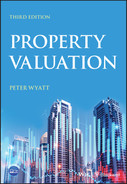
The value of a piece of land (or site) will depend not only on its existing use but also on its potential for alternative uses, including its development potential – referred to as development land value. The residual method is used to estimate development land value. It involves estimating the value of the proposed completed development using the market approach or income approach, and then deducting all the costs of the development, including profit for the developer, leaving a residual development land value. The basic equation is:

For the development of a particular piece of land or site to be economically viable, the value of the completed development less all expenditure on land, construction and profit, must exceed existing use value.
Although widely used to estimate development land value, the residual method (and the equation above) can be adapted to estimate the level of potential profit. In this way, the residual method becomes a means of assessing development viability as well as estimating land value.
The need for development arises in three situations; where new buildings are to be created on previously undeveloped land (new development), where existing buildings on vacant/derelict sites are to be replaced by new structures (redevelopment) and where existing buildings are to be substantially converted or modernised (refurbishment). For the purposes of explaining the residual method, the generic term development will be used for all these situations. Redevelopment sites compete with new development sites for potential uses. New development sites may have the advantage of being clear of any previous development, but redevelopment sites often benefit from existing infrastructure and services.
Development activity is a highly visible, often intrusive process that is responsible for creating a landscape that influences the way that we interact with each other and with the built and natural environment. But here we focus on the financial economics of development because that is where valuation fits in to the process of development. Development land valuations differ markedly from other areas of valuation, principally because the subject of the valuation is a proposal for a development rather than an extant property. For this reason, obtaining comparable evidence of development land values can be very difficult. Each site will differ widely in terms of size, condition, potential use or uses, permitted density of development, restrictions and so on, making any adjustment to a standard value per hectare almost impossible. Instead, a valuer will frequently rely on comparable evidence to assess development value and costs.
The residual method is usually employed in two ways, a basic residual and a discounted cash flow. A basic residual is simple, quick to do and easy to interpret. A cash flow provides a detailed breakdown of income and expenditure as the scheme progresses from inception to fruition. Cash‐flow techniques are useful because, once the initial feasibility has been established, a more detailed financial appraisal is usually required not only by the developer but also by the lender (who may be financing the development) and the investor (who may be acquiring the scheme on completion). Being able to identify the cash flow at any point in time during a development project has obvious advantages over the ‘snap‐shot’ estimate produced by a basic residual valuation.
8.3.1 Basic residual technique
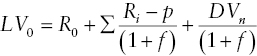
The basic residual technique can be summarised as follows:
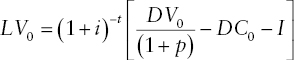
whereLV 0 = Present residual land value
- i = Cost of finance (annual interest rate)
- t = Development period (years)
- DV 0 = Current estimate of development value
- p = Profit, calculated as a percentage of DV
- DC 0 = Current estimate of development costs
- I = Finance costs (usually calculated over the construction phase of the development period only)
The model produces a simplified representation of the financial flows in development based on the following assumptions:
- The development value, expressed in current values, is received at the end of the development period.
- All development costs (land and construction) are debt financed with repayment in full at the end of the development period.
- Building costs are incurred evenly throughout the construction period and interest is calculated by halving the time over which interest accrues. The use of the finance rate effectively delays payment for the costs of development to the end of the development, placing them at the same date at which development value is received.
- Profit is deducted as a cash lump sum, taken as a proportion of total development costs or development value. As profit is also a cost to the development at the end of the development, all the income and outgoings are now placed at the end.
- Finally, the gross residual amount is the amount that can be paid for the site at the end of the development. But site value is a present value and therefore the residual surplus at completion of the development is discounted back from the end of the development to the beginning at the finance rate. Consequently, it is assumed that the land value is paid to the landowner at the commencement of the development and is funded entirely by debt.
An example of a basic residual valuation is shown below. This is an office scheme, and the relevant steps of the valuation are explained below the valuation.
| Inputs | |
|---|---|
| Areas | |
| Gross internal area (GIA) (m2) | 2000 |
| Efficiency ratio (net/gross area) | 85% |
| Net internal area (NIA) (m2) | 1700 |
| Time | |
| Lead‐in period (years) | 0.25 |
| Building period (years) | 1.50 |
| Void period (years) | 0.25 |
| Values | |
| Estimated rental value (ERV) (£/m2) | 200.00 |
| Net initial yield | 7.00% |
| Costs | |
| Site preparation (£) | 25 000 |
| Building costs (£/m2 GIA) | 969 |
| External costs (£) | 120 000 |
| Professional fees (% building costs and external works) | 13.00% |
| Miscellaneous costs (£) | 80 000 |
| Contingency allowance (% construction costs) | 3.00% |
| Planning fees (£) | 5000 |
| Building regulation fees (£) | 20 000 |
| Planning obligations (£) | 0 |
| Other fees, e.g. legal, loan, valuation (£) | 95 238 |
| Short‐term finance rate (annual) | 10.00% |
| Short‐term finance rate (quarterly) | 2.41% |
| Letting agent's fee (% ERV) | 10.00% |
| Letting legal fee (% ERV) | 5.00% |
| Marketing (£) | 10 000 |
| Sale costs (% NDV) | 2.00% |
| Land purchase costs (% site purchase price) | 6.50% |
| Developer's profit (% costs): | 20.00% |
| Basic residual land valuation | ||||
|---|---|---|---|---|
| Development value | ||||
| Net internal area (NIA) (m2) | 1700 | |||
| Estimated rental value (ERV) (£/m2) | 200 | |||
| 340 000 | ||||
| Net initial yield | 7.00% | 14.2857 | ||
| Gross development value (GDV) before sale costs (£) | 4 857 143 | |||
| Net development value (NDV) after sale costs (£) | 4 761 905 | |||
| Development costs | ||||
| Site preparation (£) | (25 000) | |||
| Building costs (£/m2 GIA) | 969 | (1 938 000) | ||
| External costs (£) | (120 000) | |||
| Professional fees (% building costs and external works) | 13.00% | (267 540) | ||
| Miscellaneous costs (£) | (80 000) | |||
| Contingency allowance (% construction costs) | 3.00% | (72 166) | ||
| Planning fees (£) | (5000) | |||
| Building regulation fees (£) | (20 000) | |||
| Planning obligations (£) | 0 | |||
| Other fees, e.g. legal, loan, valuation (£) | (95 238) | |||
| Interest on costs and fees for half building period @ | 10.00% | (194 359) | ||
| Interest on costs and finance for void period @ | 10.00% | (67 936) | ||
| Letting agent's fee (% ERV) | 10.00% | (34 000) | ||
| Letting legal fee (% ERV) | 5.00% | (17 000) | ||
| Marketing (£) | (10 000) | |||
| Developer's profit on total development costs (%): | 20.00% | (589 248) | ||
| Total development costs (TDC) (£) | (3 535 486) | |||
| NDV − TDC (£) | 1 226 418 | |||
| Land costs (£) | ||||
| Developer's profit on land costs (%) | 20.00% | (204 403) | 1 022 015 | |
| Finance on land costs over total development period | 10.00% | 2.00 | 0.8264 | |
| Residual land value before purchase costs (£) | 844 641 | |||
| Residual land value after purchase costs @ 6.5% (£) | 793 090 |
8.3.1.1 Development value
Buildings should be measured in accordance with appropriate International Property Measurement Standards (IPMS). The gross internal area of the building to be developed (the area contained within the perimeter walls of the building) is the IPMS2 area (see Chapter 6). The net internal area, or IPMS3 area, is that part of the building on which rent can be charged and excludes corridors, plant rooms, lift lobbies, toilets, etc. Some properties such as supermarkets and industrial buildings are let on an IPMS2 basis while offices and shops are let on an IPMS3 basis, with shops being zoned to reflect the higher value attached to floor area (or sales space) nearer the front of the premises. The ratio of the IPMS2 to IPMS3 areas is called the efficiency ratio. The more efficient a building, the more space there is to charge rent on. Higher efficiency ratios lead to higher annual rentals per unit of constructed space. In practice, comparable properties would be examined to determine an appropriate efficiency ratio.
The market rent is estimated by considering rents that have been achieved on comparable properties. A net rent should be estimated that has been reduced to account for any regular expenditure such as management, repairs, or insurance. It is usual practice to estimate current rent rather than predict the rent that might be achieved when the development is complete.
The gross development value (GDV) is the price for which the completed development could be sold. For commercial property, GDV is calculated by undertaking an investment valuation based on the capitalisation of expected annual rent at an appropriate yield. For residential property, GDV would be based on estimated sale prices.
The price that an investor would be prepared to pay for the completed development would be net of any purchase costs such as legal fees and surveyor's fees. If the completed development is to be retained as an investment, it will usually need to be refinanced (perhaps by converting the short‐term development loan into a long‐term debt) and it is assumed that the lender will charge an arrangement fee together with the costs of a valuation of the investment. A percentage deduction is therefore made from GDV to reflect these costs and to arrive at a net development value (NDV).
8.3.1.2 Construction costs
An estimation of the construction costs, at the valuation date, is a major component in a residual valuation. In other than the most straightforward schemes, it is recommended that the costs be estimated with the assistance of an appropriately qualified expert. Care is to be taken to check that calculations provided by other professionals are on a consistent measurement basis, i.e. IPMS.
Site preparation costs can include:
- The cost of meeting environmental requirements;
- Remediation of contamination, noise abatement and emissions controls;
- Ground improvement works;
- Archaeological investigations;
- Diversion of essential services and highway works and other off‐site infrastructure;
- Creating the site establishment and erection of hoardings;
- Conforming to health and safety regulations during the development;
- Realistic allowances for securing vacant possession, acquiring necessary interests in the subject site, extinguishing easements or removing restrictive covenants, rights of light compensation, party wall agreements, etc., reflecting that other parties expect to share in development value generated
Building costs and fees are usually estimated by a quantity surveyor, but an approximation can be gained by reference to recent contracts for similar developments or from building price books. It is usual to use current cost estimates and assume that cost inflation will match rental growth over the development period. Having said this, it is worth noting that construction contracts vary; they may be agreed on a ‘rise and fall’ or ‘fixed‐price’ basis. A building contractor who agrees to a fixed‐price contract is likely to charge a higher price because risk exposure is greater. Also, a fixed price contract is only fixed to the extent of the works outlined in the contract. A contractor can amend the pricing if any variations to the specification are made or unforeseen events occur.
External works might include demolition, access roads, car parking, landscaping, ground investigations or other costs associated with the development that are in addition to the unit price building cost estimated above.
Professional fees are usually agreed as a percentage of the construction costs but may be a fixed sum. Marshall and Kennedy (1993) found that a typical total for fees averaged 14.5%; Table 8.1 shows a representative breakdown of these fees. The appropriate fee level depends on the type and location of the development. The following items may need consideration linked to the sale, letting, design, construction, and financing of the development (RICS 2019):
Table 8.1 Typical professional fee levels.
| Professional | Fee as a % of building costs |
|---|---|
| Architect | 5–7.5% |
| Quantity surveyor | 2–3% |
| Structural engineer | 2.5–3% |
| Civil engineer | 1–3% |
| Project manager | 2+ % |
| Mechanical and electrical consultants | 0.5–3% |
- Professional consultants to design, cost and project manage the development. A development team normally includes: an environmental and/or planning consultant, an architect, a quantity surveyor and a civil and/or structural engineer. Additional specialist services may be supplied as appropriate by mechanical and electrical engineers, landscape architects, traffic engineers, acoustic consultants, project managers and other disciplines depending on the nature of the development.
- Fees incurred in negotiating or conforming to statutory requirements (for example building consents) or any planning agreements.
- Costs related to the raising of development finance (including the lender's monitoring fees and legal fees).
- In some cases, the prospective tenant/purchaser may incur fees on monitoring the development (these may have to be reflected as an expense where they would normally be incurred by the developer).
- Lettings and sales expenses where the development is not pre‐sold or fully pre‐let. These expenses usually include incentives, promotion costs and agents' commissions. The cost of creating a ‘show’ unit in a residential development may also be appropriate.
- Incentives on letting such as fitting out periods, rent‐free periods and capital payments to prospective tenants. These may be reflected by either continuing interest charges on the land and development costs until rent commencement or taking account of the costs in the valuation of the completed development.
- Legal advice and representation at any stage of the project.
In this example, professional fees of 13% of building costs and external works have been assumed, broken down as: Project Manager (2%), Quantity Surveyor (3%), Mechanical and Electrical Engineer (1%), Structural Engineer (1%) and Architect (6%). Miscellaneous costs are included as a catch‐all for any other incidental expenditure such as insurance.
It is normal to include a contingency allowance for any unexpected increases in costs. The quantum, which is usually expressed as a percentage of building costs, is dependent upon the nature of the development, the procurement method and the perceived accuracy of the information obtained. However, whether a contingency allowance is appropriate is linked to the analysis of risk within development schemes. A contingency allowance could inadvertantly double‐count risk associated with development costs if that risk has allowed for in the developer's profit margin. Unforeseen increases in costs are an inherent risk in development and higher development returns are required to compensate for risks such as these. Therefore, a higher contingency allowance should be compensated by a relatively lower developer's profit.
The contingency allowance is a reserve fund to allow for any increase in costs or delays in construction. As construction costs are the single largest sum after land, any inflationary effect is likely to have a significant impact on costs. If the economy is particularly volatile, a cautionary approach is to apply the contingency allowance to all costs, including finance costs, but this will depend on the perceived risk of the project. Marshall and Kennedy (1993) found that a contingency fund is generally set at 3–5% of building costs and professional fees (and sometimes interest payments), but the figure varied depending on the nature of site (restrictive site, subsoil, etc.) and the development project itself. Generally, the longer the development period and the more complex the construction of the building, the higher the risk of unforeseen changes and, therefore, the higher the contingency allowance.
Regulatory fees might include planning fees, building regulation fees and the costs associated with legally binding conditions linked with the grant of development consent.
8.3.1.3 Cost of finance
Short‐term finance is usually included in valuations of development land because development typically requires debt finance. The cost of finance depends on two factors, the interest rate and the duration of the loan. A lender will charge interest at the bank base rate for lending plus a return for risk. The magnitude of the risk premium will depend on the nature of the scheme, the status of developer, the size and length of loan and the amount of collateral the developer intends to contribute.
The duration of the loan depends on the estimated length of the development period. In simple terms, the development period comprises a lead‐in period, the construction period, and a void period. The lead‐in period allows time for obtaining planning consent, preparing drawings and so on. The void period sits between the end of the construction period and occupation by a tenant, including a possible rent‐free period. During a void period, interest is payable on all costs so any extensions to this period will significantly increase the amount of loan finance incurred. In this example, a lead‐in period of 3 months, a construction period of 18 months and a void period of 3 months has been assumed.
Interest payments on money borrowed to fund construction usually accrue monthly but are rolled up over the development period and paid back when the development is let or sold. In a basic residual valuation, finance is assumed at 100% of all construction and land‐related costs. This is achieved by compounding interest on the construction costs over the construction period and by discounting the residual land value at the interest rate over the development period. Whereas finance is calculated on the land‐related costs over the development period, because finance is not drawn on all construction costs at the start of the construction period, one of three techniques is usually employed to calculate the finance on the construction‐related costs. The first is to set out the costs as a cash flow and determine the total interest payment. This technique requires a quarterly or monthly breakdown of construction costs and, for a basic residual valuation, this might seem too detailed. Therefore, an averaging technique is often employed by assuming that either interest accumulates on half the construction‐related costs over the whole construction period, or that all construction costs are borrowed over half the construction period (the approach used in this example). This averaging of either cost or time reflects the fact that interest is not paid on the full amount over the entire building period. Usually costs start off low, peak in the middle and then tail off towards the end as illustrated in Figure 8.2. By averaging, a straight line rather than an s‐shaped build‐up of costs is assumed. Sometimes, interest on professional fees is calculated separately by compounding the amount over two thirds of the building period. This reflects the presumption that such fees tend to be incurred early in the development, during the planning and design phase and hence interest will be incurred for a longer period.
It is usual for interest to be treated as a development cost up to the assumed letting date of the last unit unless a forward sale agreement dictates otherwise. If an assumption is made that the completed development is held beyond the date of completion, the costs of holding that building during this void period must be added. These may include insurance, security, cleaning and energy costs. A proportion of the service charge on partially let properties may have to be included together with any potential liability for empty property taxes. Interest can then be accumulated in two parts; in the construction period as indicated above and then in the post construction void period, where the full costs of development can be included in the interest calculations. Interest accrued during the void period is calculated by compounding the total construction costs and interest rolled up during the construction period at the annual interest rate. A significant amount of interest can accrue during a void period. That is why it is very important to keep the length of any void period to a minimum. Detailed cash‐flow projections are essential once the project is under way to incorporate changes in revenue and costs and particularly so for phased developments.
Figure 8.2 Build‐up of costs over time.
8.3.1.4 Letting and sale fees
The fees that agents and solicitors charge for either letting the completed development are usually calculated as a percentage of the estimated market rent. If the space is to be sold on a freehold or long leasehold basis (residential apartments for example), the fees are usually quoted as a percentage of sale price. The fee that agents charge will vary depending on whether they have been given sole or joint marketing rights. Marketing costs would cover items such as advertising, opening ceremony, brochure design and production and would obviously depend on the nature of the development.
8.3.1.5 Developer's profit
Developer's profit is the reward for initiating and facilitating the development and is dependent upon the size, length and type of development, the degree of competition for the site and whether it is pre‐let or sold before construction is complete (a forward sale). Property development is perceived as riskier than investment in completed and let properties. Consequently, the required return will be higher than these ‘standing’ property investments. It is usual to express developer's profit in the basic residual valuation as a cash sum, expressed as a percentage of the development cost (including finance and land costs) or of development value.3 A typical range of profit as a percentage of costs is 15–25%. Here, 20% has been assumed.
The developer also takes a profit margin on the residual land costs. The equation below shows how this is calculated.
8.3.1.6 Residual land costs
Once developer's profit has been deducted from the residual land costs, the remaining sum must cover the land price, purchase costs and finance on these costs. These are handled in reverse order. Regarding finance, assuming the site was purchased by the developer at the start of the development, interest on land costs will accrue over the total development period. To reflect this, the residual land costs are discounted at the short‐term finance rate of 10% over the total development period to determine their present value.4
Acquisition costs are deducted to leave the net amount remaining for purchase of the land. These acquisition costs usually include legal costs, transfer tax or Stamp Duty agents' fees:
The final figure is the residual land value and represents the maximum amount that should be paid for the site if the proposed development was to proceed and all the valuation assumptions held true.
8.3.2 Basic residual profit appraisal
Given all the value and cost inputs, including a developer's profit margin, the output from the residual method is usually a land valuation. However, if a land price is one of the cost inputs, then the method can be used to estimate the amount of developer's profit.
In a basic residual, if the land price or value is known, it becomes a cost to the development. It occurs at the beginning of the development and interest accrues on it over the development period. This cost is added to the other development costs and then deducted from development value to leave an estimate of residual profit at the end of the development period.
The basic equation for the residual land valuation can be transposed to determine the level of profit achieved given construction and site costs. The equation would look like this:
| Value of completed development – development costs (including developer’s profit) = Development land value |
| Less development costs, including site price |
| Equals developer's profit |
Using the example above, the estimation of developer's profit would proceed as follows.
| Basic residual profit appraisal | |||
|---|---|---|---|
| Development value | |||
| Net internal area (NIA) (m2) | 1700 | ||
| Estimated rental value (ERV) (£/m2) | 200 | ||
| 340 000 | |||
| Net initial yield | 7.00% | 14.2857 | |
| Gross development value (GDV) before sale costs (£) | 4 857 143 | ||
| Net development value (NDV) after sale costs (£) | 4 761 905 | ||
| Development costs | |||
| Land price (£) | (793 090) | ||
| Land purchase costs (% land price) | 6.50% | (51 551) | |
| Finance on land costs for total development period @ | 10.00% | (177 375) | |
| Site preparation (£) | (25 000) | ||
| Building costs (£/m2 GIA) | 969 | (1 938 000) | |
| External costs (£) | (120 000) | ||
| Professional fees (% building costs and external works) | 13.00% | (267 540) | |
| Miscellaneous costs (£) | (80 000) | ||
| Contingency allowance (% construction costs) | 3.00% | (72 166) | |
| Planning fees (£) | (5000) | ||
| Building regulation fees (£) | (20 000) | ||
| Planning obligations (£) | 0 | ||
| Other fees, e.g. legal, loan, valuation (£) | (95 238) | ||
| Finance on building costs and fees for HALF building period @ | 10.00% | (194 359) | |
| Finance on building costs, fees and interest to date for void period: | 10.00% | (67 936) | |
| Letting agent's fee (% ERV) | 10.00% | (34 000) | |
| Letting legal fee (% ERV) | 5.00% | (17 000) | |
| Marketing (£) | (10 000) | ||
| Total development costs (TDC) (£) | (3 968 254) | ||
| Developer's profit on completion (£) | 793 651 | ||
| Return on costs | 20.00% | ||
| Return on NDV | 16.67% | ||
| Income yield | 8.57% |
The site price is assumed or is known and can therefore be inserted. Costs associated with site acquisition (typically agent and legal fees) must be added to the costs. Assuming the site was acquired at the very start, interest will accrue on this cost over the whole development period. Here the site costs will incur interest for two years at an annual interest rate of 10%.
The estimated developer's profit can be expressed in several ways to assess the viability of the development and to compare it to other development opportunities. Profit as a percentage of development costs is useful for merchant developers, who need to sell the completed development to raise capital for future projects. Some developers, particularly housebuilders, prefer to express profit as a percentage of value. Development yield is rent expressed as a percentage of development costs and is useful for investor developers who, in contrast to trader developers, retain the development as an investment. Just as the difference between total costs and total capital value represents capital profit, so the difference between the investment yield and development yield represents the developer's annual profit margin over standing investments.
8.3.3 Discounted cash‐flow technique
The discounted cash‐flow technique requires period‐by‐period assumptions concerning the breakdown of costs and values during the development period such as the time frame (monthly, quarterly, etc). It thus allows market dynamics through time to be incorporated, such as changes in costs and values, where appropriate. The basic application of a discounted cash flow is to calculate the present residual land value of the estimated costs and revenues over the duration of the development scheme. With all other costs and revenues accounted for, profit is incorporated as a cash sum, usually estimated as a percentage of total costs or revenue.
Whereas a basic residual valuation is often used at an early stage to provide a snapshot of development feasibility, a cash flow provides a more detailed assessment, usually reserved for larger, more‐complex proposals. Projecting a cash flow is particularly useful for developments where the initial land acquisition or disposal of the completed development is phased, such as residential or industrial estates, where some units may be sold before others are constructed, or complex central area shopping schemes where parts may be let or sold before the remainder is complete. In short, the advantage of the cash‐flow technique is its dynamic capability.
The essential difference between a basic residual valuation and a cash‐flow valuation is the way that the timing of expenditure and revenue is handled. The basic residual assumes that revenue from the development is received at the end of the development and interest on expenditure is calculated on 50% of all costs over the building period (alternatively, interest is calculated on the total costs over half of the building period). In contrast, a cash flow divides the development project into time periods (usually months or quarters) to allow more refined judgements to be made regarding the flow of income and expenditure. Payments and receipts that were stated as aggregate figures in the residual valuation may now be estimated as to when they are likely to occur. This permits a more accurate calculation of interest payments to be incorporated and allows the valuer to examine how changes in the timing of costs and revenue might affect value or profitability of the development. Throughout the construction phase, adjustments can be made to the cash flow as and when costs and income are realised. This will determine how the project stands at any point in time in terms of potential profit and what began as a valuation becomes an appraisal tool. In a basic residual, it is usually assumed that income is received (and costs incurred) annually in arrears. A cash flow typically assumes that costs and revenue are incurred and received quarterly in arrears. There may be a mixture of timings for incurring expenditure and receiving revenue: construction costs are usually paid in arrears whereas income from property in the form of rent is usually receivable quarterly in advance.
A key advantage of a cash‐flow valuation is that it can deal with non‐standard patterns of revenue and expenditure. Whereas a basic residual valuation assumes sales must come at the end of the development (albeit after a possible void period), the cash‐flow method easily deals with phased schemes, allowing rental income to be accounted for when rent commences before the investment is sold. For example, the leasing of advertising space on hoardings or securing short‐term tenancies (for example surface car parking) can help to offset costs before and during the development phase. This is simple to include by incorporating two income lines: one for rent and one for sales. Where phased sales occur, the associated costs, such as agent and legal fees, should also appear in the calculation at the appropriate time. Also, when the opening balance becomes positive, no interest should be charged.
The basic approach of the discounted cash‐flow approach can be formalised as follows:
where R = Recurring periodic net revenue received at the end of each period, f = cost of finance, n = number of periods and other variables are as defined above.
In this simple cash‐flow valuation, revenue and expenditure are discounted at the finance rate and developer's profit is included as a cash sum at the end. This is the same as the approach adopted in the basic residual, but a cash flow means that where revenue is expected to be received in phases, receipts can be recognised in the cash flow at the appropriate time. Phasing may be appropriate for residential development where homes are built and sold incrementally or for commercial developments where some existing properties are let on a short‐term basis while new properties are built. The timing and extent of phased costs and revenue within the development period can be incorporated into the cash flow. Where income‐producing properties are included in the development, the timing of lettings, rent‐free periods, capital contributions, etc., can also be incorporated into the cash flow and the development period can be extended as necessary.
Using the example from above, the cash flow below replicates the input costs but allocates them across the development period in a more realistic way. The land price is input at the start, construction costs and fees are spread over the eight quarters and developer's profit is paid out at the end. Discounting the cash flow at the finance rate leaves a small negative net present value (NPV). Whereas the basic residual assumed all costs were incurred at the halfway point, in the cash flow, the spread of costs is weighted a little before the halfway point. This leads to slightly higher finance costs and thus a small negative closing balance of ‐£46 408. This would eat into the developer's profit. To see how much the developer should reduce the land bid price to preserve the profit margin, the higher finance cost can be fed back into a revised land valuation using iteration (‘goal seek’ in Excel) to set the closing balance to zero and altering the land price input. The revised land price is £757 077.
| Cash‐flow residual land valuation | ||||||||||
|---|---|---|---|---|---|---|---|---|---|---|
| Total | 0 | 1 | 2 | 3 | 4 | 5 | 6 | 7 | 8 | |
| Development value | ||||||||||
| Net development value (NDV) after sale costs (£) | 4 761 905 | 0 | 0 | 0 | 0 | 0 | 0 | 0 | 0 | 4 761 905 |
Development costs | ||||||||||
| Land price (£) | (793 090) | (793 090) | 0 | 0 | 0 | 0 | 0 | 0 | 0 | 0 |
| Land purchase costs (% land price) | (51 551) | (51 551) | 0 | 0 | 0 | 0 | 0 | 0 | 0 | 0 |
| Site preparation (£) | (25 000) | (25 000) | 0 | 0 | 0 | 0 | 0 | 0 | 0 | 0 |
| Building costs | (1 938 000) | 0 | 0 | (387 600) | (581 400) | (775 200) | (193 800) | 0 | 0 | 0 |
| External costs (£) | (120 000) | 0 | 0 | (60 000) | (60 000) | 0 | 0 | 0 | 0 | 0 |
| Professional fees | (267 540) | 0 | 0 | (160 524) | (107 016) | 0 | 0 | 0 | 0 | 0 |
| Miscellaneous costs (£) | (80 000) | 0 | 0 | 0 | 0 | 0 | (80 000) | 0 | 0 | 0 |
| Contingency allowance (% construction costs) | (72 166) | 0 | 0 | (18 244) | (22 452) | (23 256) | (8214) | 0 | 0 | 0 |
| Planning fees (£) | (5000) | (5000) | ||||||||
| Building regulation fees (£) | (20 000) | (20 000) | ||||||||
| Other fees, e.g. legal, loan, valuation (£) | (95 238) | (95 238) | ||||||||
| Marketing (£) | (10 000) | 0 | 0 | 0 | 0 | 0 | 0 | 0 | 0 | (10 000) |
| Letting agent's fee (% ERV) | (34 000) | 0 | 0 | 0 | 0 | 0 | 0 | 0 | 0 | (34 000) |
| Letting legal fee (% ERV) | (17 000) | 0 | 0 | 0 | 0 | 0 | 0 | 0 | 0 | (17 000) |
| Developer's profit (% NDV) | (793 651) | |||||||||
| Net cash flow before finance | (869 641) | 0 | (626 368) | (770 868) | (798 456) | (402 252) | 0 | 0 | 3 907 254 | |
Finance | ||||||||||
| Opening balance (£) | 0 | (869 641) | (890 611) | (1 538 455) | (2 346 421) | (3 201 458) | (3 680 909) | (3 769 669) | (3 860 570) | |
| Interest (in arrears) (£) | (486 077) | 0 | (20 970) | (21 476) | (37 098) | (56 581) | (77 199) | (88 760) | (90 901) | (93 093) |
| Closing balance (£) | (869 641) | (890 611) | (1 538 455) | (2 346 421) | (3 201 458) | (3 680 909) | (3 769 669) | (3 860 570) | (46 408) | |
Iteration can also be used to determine how the developer's profit might change if the land price had to remain at £793 090. In this case, the profit sum drops to £747 242.
In practice, developers rarely if ever use 100% debt to finance land acquisition and construction. A cash flow can be used to consider various finance arrangements and loan to cost ratios. In doing so, the cash flow is constructed on the equity provided by the developer and the target rate of return is based on the risk of that equity. Depending upon the financial arrangements, that risk would normally be higher than the overall project risk (this assumes lower risk exposure by the lender) and the equity target rate of return would normally be in excess of the project target rate of return.
To summarise, there is a great deal of uncertainty in the residual method. Although there may be a predictable set of costs associated with parts of a development project, there will inevitably be unforeseen costs and delays. Typically, these are handled by a contingency allowance and a suitable risk‐adjusted profit margin for the developer. Nevertheless, given very high yet relatively predictable costs (building, fees, finance, etc.) and more volatile revenue (sale prices, rents, yields, letting voids, etc.), developers face high operational gearing. Most projects are lengthy, and costs, values and market activity will change during the development time frame. Little forecasting is undertaken in residual land valuations so this presents additional risk to the developer. Because of inherent uncertainty in the model and the highly geared nature of the residual land value, the method comes with two major health warnings: it is highly site specific and has a very limited shelf‐life.
References
- Marshall, P. and Kennedy, C. (1993). Development valuation techniques. J. Prop. Valuat. Invest. 11 (1): 57–66.
- RICS (2019). RICS Professional Standards and Guidance, Global, October 2019: Valuation of Development Property, 1e. London: Royal Institution of Chartered Surveyors.
- Scarrett, D. (1991). Property Valuation: The 5 Methods. London: Spon Press.
- Whipple, R. (1995). Property Valuation and Analysis. Sydney: The Law Book Company.
Questions
Replacement cost method
- A local authority owns a recycling centre that must be valued for their register of assets. The property is expected to have a further 25 years of useful life remaining from its original life expectancy of 40 years. The building comprises 5000 square metres gross internal area and construction costs are estimated at £1098 per square metre. A replacement building and compound would take 9 months to construct, fees are estimated at 12% and the local authority could be expected to secure finance at 4.5%. The building is located on a site comprising 18 000 square metres and the price of land per hectare (per 10 000 square metres) for refuse and recycling centre use is estimated at £18 500. Value the freehold of the building.
- A purpose‐built glass works comprises specialised industrial buildings, a warehouse, canteen and office accommodation, details of which are shown in the schedule below. The property has been developed over several years on a site comprising 2.5 ha. Market evidence shows that current land values are approximately £52 000 per hectare for heavy industrial use.
Building description Life expectancy Remaining useful life Gross replacement cost (including fees and finance per building) Main glass works 60 20 £6 000 000 Laboratory 60 20 £1 000 000 Canteen and offices 30 5 £800 000 Warehouse 60 40 £9 000 000 - Assuming a replacement building would take 21 months to reinstate, and that the owner could secure a finance rate of 7% per annum, value the freehold interest.
- If you were aware that the main glass works building had an inefficient layout for modern manufacturing methods, how might you adjust your valuation?
- If you were aware that modern manufacturing plants to replace this building would now be located on a site comprising 1.75 ha, how might you adjust your valuation?
Residual method
- You have been asked to value an office development site based on the following assumptions:
- Gross internal area of 5000 square metres and an efficiency ratio of 85%.
- The market rent is estimated to be £200 per square metre and the investment yield 6%.
- Building costs are £1200 per square metre, external works £250 000 and ancillary costs £200 000.
- Lead in period: 0.50 years, building period: 1.50 years, void period: 0.75 years
- Professional fees are estimated to be 10% of building costs and external works.
- There is a contingency allowance of 3% of building costs, external works, ancillary costs and professional fees.
- Other costs and fees include site investigations of £10 000, planning application fees of £5000, building regulations of £20 000.
- Finance can be arranged at a rate of 7% per annum.
- The letting agent fee is 10% of the ERV and the letting legal fee is 5% of the ERV. The marketing budget is £150 000.
- Developer's profit is 15% of all development and land costs.
- A property development company is proposing to develop an office building on a recently acquired town‐centre site. The purchase price was £1.6m and the previous owner had obtained outline planning consent for a four‐storey building on the site some two years previously but had not pursued this proposal. A local commercial letting agent has indicated that demand for office space in the town is high and leases have recently been negotiated at rental levels of £220 per square metre per annum. The agent is not aware of any other new office development proposals in the town. Recent investment transactions show capitalization rates around 8%. The developer has appointed local architects and surveyors and, on the basis of their knowledge, the architect has drawn up a design that provides a building with a gross internal area of 4667 square metres. Analysis of the design shows that the efficiency ratio will be 90%. The developer's agent reports that, among other expressions of interest, they have received firm enquiries from several tenants about leasing space in the development. The quantity surveyor has indicated that building costs for good‐quality speculative offices are expected to be £1075 per square metre. External works are expected to cost approximately £250 000 and a separate contract has already been let for site clearance and the demolition of some small buildings on the site at a price of £100 000. The project manager has drawn up an outline procurement programme that allows six months for design, 15 months for construction and a six‐month letting void. The developer intends to borrow the cost of the development from a bank. Current interest rates on project loans of this nature are around 8% per annum. Calculate the developer's profit and report it as a cash sum, as a percentage of costs and as a percentage of value.
- Estimate the residual land value from the following net cash flow, assuming a finance rate of 10% per annum.
Quarter 0 1 2 3 4 5 6 Net cash flow (138 284) (500 000) (500 000) (500 000) (500 000) (500 000) 4 000 000 - Estimate the residual land value from the following development revenue and expenditure items over a one‐year development period, assuming a finance rate of 10% per annum.
Quarter 1 2 3 4 Sales 0 0 300 000 300 000 Construction (25 000) (25 000) (25 000) (25 000) Demolition (20 000) 0 0 0 Prof. fees (2250) (1250) (1250) (1250) Sale fees 0 0 (4500) (4500) Contingency (2363) (1313) (1538) (1538) Profit (120 000) - Estimate the residual land value of the following development cash flow. The development has a gross internal area of 900 square metres and an efficiency ratio of 80%. Site clearance costs of £100 000 are anticipated in Q1. Building costs are £900 per square metre, with 25% due in Q2, 50% in Q3 and 25% in Q4. Professional fees are 10% of building costs and contingencies are 5% of building costs and professional fees. A simultaneous letting and sale is anticipated in Q7. The MR is estimated to be £220 per square metre, the yield 6%, letting fee 10% of MR and sale fee 2% of NDV. Developer's profit is 17% of GDV and finance can be arranged at a cost of 8% per annum.
- Estimate the developer's profit from the following inputs. Assume that the build costs are spread evenly between Q2 and Q5.
INPUTS Land price (£) 850 000 Yield 7.00% Gross internal area (m2) 2000 Efficiency ratio 90% Build cost (£/m2) 1000 Estimated MR (£/m2) 175 Land purchase costs (% land price) 5.75% Investment sale fee (% NDV) 5.75% Letting fee (% MR) 10% Lead‐in period (quarters) 1 Building period (quarters) 4 Void period (quarters) 2 Contingencies (% build costs and fees) 5% Professional fees (% build costs) 10% Finance rate (per quarter) 2.00%
Answers
Replacement cost method
Building area (m2) 5000 Building cost (£/m2) 1098 Cost of modern equivalent building (£) 5 490 000 Fees (% build cost) 12% 658 800 Finance on build cost and fees over half build period @ 4.50% 102 336 Gross replacement cost of building (£) 6 251 136 Depreciation allowance (age/estimated economic life) 38% Net replacement cost of building (£) 3 906 960 Site area (ha) 1.80 Land value (£/ha) 18 500 Value of land (£) 33 300 Finance on land over build period @ 4.50% 1118 Cost of land (£) 34 418 Valuation before PCs (£) 3 941 378
a)Main glass works Gross replacement cost inc. fees and finance (£) 6 000 000 Depreciation allowance (% remaining life) 20 60 33% Net replacement cost (£) 2 000 000 Laboratory Gross replacement cost inc. fees and finance (£) 1 000 000 Depreciation allowance (% remaining life) 20 60 33% Net replacement cost (£) 333 333 Canteen and offices Gross replacement cost (inc. fees and finance) 800 000 Depreciation allowance (% remaining life) 5 30 17% Net replacement cost (£) 133 333 Warehouse Gross replacement cost (inc. fees and finance) 9 000 000 Depreciation allowance (% remaining life) 40 60 67% Net replacement cost (£) 6 000 000 Land Site area (ha) 2.5 Estimate value (£/ha) 52 000 130 000 Finance on land cost (FV £1 for 1.75 years at 7% p.a.) 1.75 7.00% 1.1257 146 341 Replacement cost valuation (£) 8 613 007 b) A further percentage deduction might be made in addition to the straight‐line depreciation charge made on the main chemical works due to its size.
c) Recalculate the land costs based on 1.75 ha. Also consider if the remaining hectare has an alternative use value and could be valued separately to reflect any development land value.
Residual method
INPUTS Areas Gross internal area (GIA) (m2) 5000 Efficiency ratio (net/gross area) 85% Net internal area (NIA) (m2) 4250 Time Lead‐in period (years) 0.5 Building period (years) 1.5 Void period (years) 0.75 Values Estimated rental value (ERV) (£/m2 NIA) 200 Net initial yield 6.00% Costs Site preparation (£) 10 000 Building costs (£/m2 GIA) 1200 External works (£) 250 000 Professional fees (% construction costs and external works) 10% Miscellaneous costs (£) 200 000 Contingency allowance (% of all construction costs) 5.00% Planning fees (£) 5000 Building regulation fees (£) 20 000 Planning obligations (£) 0 Other fees, e.g. legal, loan, valuation (£) 0 Short‐term finance rate (annual) 7.00% Letting agent's fee (% ERV) 10% Letting legal fee (% ERV) 5% Marketing (£) 150 000 Sale costs (% NDV) 2.00% Land purchase costs (% land price) 6.50% Developer's profit (% development costs) 15.00% RESIDUAL LAND VALUATION Development value Net internal area (NIA) (m2) 4250 Estimated rental value (ERV) (£/m2 NIA) 200 ___________ 850 000 Net initial yield 6.00% 16.6667 Gross development value (GDV) before sale costs (£) 14 166 667 Net development value (NDV) after sale costs (£) 13 888 889 Development costs Site preparation (£) (10 000) Building costs (£/m2 GIA) 1200 (6 000 000) External works (£) (250 000) Professional fees (% construction costs and external works) 10.00% (625 000) Miscellaneous costs (£) (200 000) Contingency allowance (% of all construction costs) 5.00% (353 750) Planning fees (£) (5000) Building regulation fees (£) (20 000) Planning obligations (£) 0 Other fees (£) 0 Finance on above costs for half building period @ 7.00% (388 514) Finance on above costs for void period @ 7.00% (408 738) Letting agent's fee (% ERV) 10.00% (85 000) Letting legal fee (% ERV) 5.00% (42 500) Marketing (£) (150 000) Developer's profit on above costs @ 15.00% (1 280 775) Total development costs (TDC) (£) (9 819 278) NDV − TDC (£) 4 069 611 Land costs Developer's profit on land costs @ 15.00% (530 819) 3 538 792 Finance on land costs over total development period @ 7.00% 2.75 0.8302 _________ Residual land value before purchase costs (£) 2 937 986 Residual land value after purchase costs (£) 6.50% 2 758 672
INPUTS Areas Gross internal area (GIA) (m2) 4667 Efficiency ratio (net/gross area) 90% Net internal area (NIA) (m2) 4200 Time Lead‐in period (years) 0.50 Building period (years) 1.25 Void period (years) 0.50 Values Estimated rental value (ERV) (£/m2 NIA) £220.00 Net initial yield 8.00% Costs Land price (£) 1 600 000 Site preparation (£) 100 000 Building costs (£/m2 GIA) 1075 External works (£) 250 000 Professional fees (% construction costs and external works) 13.00% Miscellaneous costs (£) 0 Contingency allowance (% of all construction costs) 3.00% Planning fees (£) 0 Building regulation fees (£) 0 Planning obligations (£) 0 Other fees, e.g. legal, loan, valuation (£) 0 Short‐term finance rate (annual) 8.00% Letting agent's fee (% ERV) 10.00% Letting legal fee (% ERV) 5.00% Marketing (£) 0 Sale costs (% NDV) 2.00% Land purchase costs (% land price) 6.50% RESIDUAL PROFIT VALUATION Development value Net internal area (NIA) (m2) 4200 Estimated rental value (ERV) (£/m2 NIA) 220 __________ 924 066 Net initial yield 8.00% 12.5000 Gross development value (GDV) before sale costs (£) 11 550 825 Net development value (NDV) after sale costs (£) 11 324 338 Development costs Land price (£) (1 600 000) Land purchase costs (% land price) 6.50% (104 000) Finance on land costs for total development period @ 8.00% (322 157) Site preparation (£) (100 000) Building costs (£/m2 GIA) £1075 (5 017 025) External works (£) (250 000) Professional fees (% construction costs and external works) 13.00% (684 713) Miscellaneous costs (£) 0 Contingency allowance (% of all construction costs) 3.00% (178 552) Planning fees (£) 0 Building regulation fees (£) 0 Planning obligations (£) 0 Other fees, e.g. legal, loan, valuation (£) 0 Finance on above costs for half building period @ 8.00% (307 005) Finance on above costs for void period @ 8.00% (256 461) Letting agent's fee (% ERV) 10.00% (92 407) Letting legal fee (% ERV) 5.00% (46 203) Marketing (£) 0 Total development costs (TDC) (£) (8 958 524) Developer's profit on completion (NDV − TDC) (£) 2 365 814 Profit as a percentage of costs 26.41% Profit as a percentage of value (NDV) 20.89% Income yield (ERV as a percentage of costs) 10.31% - Convert 10% per annum to quarterly equivalent rate: (1.10)0.25 − 1 = 2.41% p.q.
Quarter 0 1 2 3 4 5 6 Net cash flow (£) (138 284) (500 000) (500 000) (500 000) (500 000) (500 000) 4 000 000 PV @ 2.41% 1 0.9765 0.9535 0.9310 0.9091 0.8877 0.8668 PV of cash flow (£) (138 284) (488 227) (476 731) (465 506) (454 545) (443 843) 3 467 137 NPV (residual land value before PCs) (£) 1 000 000 Residual land value after PCs @ 6.5% (£) 938 967 - Convert 10% per annum to quarterly equivalent rate: (1.10)0.25 − 1 = 2.41% p.q.
Quarter 1 2 3 4 Net cash flow (£) (49 613) (27 563) 267 712 147 712 PV @ 2.41% (48 445) (26 280) 249 243 134 284 NPV (residual land value before PCs) (£) 308 802
Inputs Gross internal area (m2) 900 Efficiency ratio 80% Build cost (£/m2) 900 Professional fees (% build cost) 10% Contingencies (% build cost and fees) 5% Rent (£/m2) 220 Yield 6.00% Investment sale fee 2.00% Letting fee (% MR) 10% Land purchase costs (% land value) 6.50% Developer's profit (% GDV) 17% Finance rate (% p.a.) 8% Calculations Estimated MR (£/m2) 158 400 Gross development value (£) 2 640 000 Net development value (£) 2 478 873 Quarterly finance rate (% p.q.) 1.94% Cash flow Quarter 1 2 3 4 5 6 7 NDV (£) 2 478 873 Site clearance (£) (100 000) Building (£) (202 500) (405 000) (202 500) Professional fees (£) (20 250) (40 500) (20 250) Contingencies (£) (11 138) (22 275) (11 138) Letting fee (£) (15 840) Developer's profit (£) (448 800) Net cash flow (£) (100 000) (233 888) (467 775) (233 888) 0 0 2 014 233 PV £1 @ finance rate 0.9809 0.9623 0.9439 0.9259 0.9083 0.8910 0.8740 PV of cash flow (£) (98 094) (225 058) (441 539) (216 563) 0 0 1 760 428 (residual land value before PCs) (£) 779 173 Residual land value after PCs @ 6.5% 731 618
Calculations Build costs (£) 2 000 000 Market rent (£ p.a.) 315 000 Gross development value (GDV) (£) 4 500 000 Net development value (NDV) (£) 4 255 319 Cash flow Quarter 0 1 2 3 4 5 6 7 TOTALS Land price (£) (850 000) Land purchase costs (% land price) (48 875) Building costs (£) (500 000) (500 000) (500 000) (500 000) Professional fees (% build costs) (50 000) (50 000) (50 000) (50 000) Contingencies (% build costs and fees) (27 500) (27 500) (27 500) (27 500) Letting fee (% MR) (31 500) (3 240 375) Net development value (NDV) 4 255 319 Net cash flow (£) (898 875) (577 500) (577 500) (577 500) (577 500) 4 223 819 Finance Opening balance (£) (898 875) (916 853) (1 512 690) (2 120 443) (2 740 352) (3 372 659) (3 440 112) Interest (arrears) (£) (17 978) (18 337) (30 254) (42 409) (54 807) (67 453) (68 802) (300 040) Closing balance (£) (898 875) (916 853) (1 512 690) (2 120 443) (2 740 352) (3 372 659) (3 440 112) 714 904 Profit sum (£) 714 904 Profit on cost 20.19% Final closing balance divided by all costs including interest Profit on GDV 15.89% Final closing balance divided by GDV Development yield 8.90% Market rent divided by costs Profit erosion by rent (years) 2.27 Closing balance divided by market rent
Notes
- 1 A generic term covering all additions to the land including services, paving, fencing, etc., even though they may have different uses and economic lives.
- 2 The economic life of a building can be thought of as that period over which it proves to be the most appropriate (least cost) built asset needed to deliver the business function. If kept beyond its economic life, a building may continue to give service, but a replacement will do the job more cost effectively.
- 3 There is a mathematical relationship between the two measures as follows:
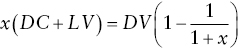
where x is > 0 and < 1
- 4 Even if money is not borrowed to fund land purchase or construction, the opportunity cost of funds used should be reflected in the valuation. In the basic residual, the interest rate is regarded as a proxy for the opportunity cost of capital.