9
Performance Metrics for Comparison of Heuristics Task Scheduling Algorithms in Cloud Computing Platform
Nidhi Rajak* and Ranjit Rajak
Department of Computer Science and Applications, Dr. Harisingh Gour Central University Sagar, M.P.
Abstract
Cloud computing is a recent demanding technology and infrastructure paradigm which is using in every field of science and technology. This technology is based on the Internet and apply one principle “pay and usage of computing resources”. Scheduling of the tasks is burning area of research in cloud, and it can be defined as the process of mapping of tasks onto the virtual machines and it should give overall minimum scheduling length that is minimize the overall execution time on cloud servers. Here, a very specific graph which is used and is called as Directed Acyclic Graph (DAG) represents of an application in the scheduling problem. A DAG is stated as the collection tasks and communication links with their value. This chapter studies four well-known heuristics of task scheduling algorithms such as HEFT, CPOP, ALAP, and PETS and finds their comparison studies based on performance metrics such as scheduling length, speedup, efficiency, resource utilization, and cost.
Keywords: DAG, upward rank, downward rank, cloud computing, speedup
9.1 Introduction
Technology is dynamic and it is changing present requirements which are prospective to future demands. Computing capability is growing at a rapid speed in every field and should be solved as fast as compared to earlier time computing technologies. Simple problems can be solved very easily using conventional systems such as sequential machines but a large or complex problem cannot easily be solved and demands high time consuming. So, to overcome this problem, many computing systems have been developed such as supercomputing but it is costly. Now, the era of cloud computing is one of the recent areas of research in the computing science field. The cost of hardware is decreasing on day to day basis and this is enforced by the use of cloud computing. A study [1] found in 2011 that cloud computing is one of the top 10 technologies for future prospective companies and organizations. The evaluation of clouds is shown in Figure 9.1 [2].
There are three aspects for evaluation of cloud as virtualization, automatic, and service-oriented architecture. The major concern of cloud computing is to better utilize of resources in the era of computing fields with optimal use of technologies. Cloud computing [1] is visible as two things such as computational paradigm and distribution architecture. There are a number of objectives [3, 4] of cloud computing platforms such as processing of the information with security and fast, providing suitable storage of data, all computation of the service over the Internet.
Scheduling of the tasks onto available resources is one of the present topics of research in cloud computing paradigm. It is formally defined as the mechanism to allocate the tasks onto the virtual machines in such a way so that overall consumption of the processing time would be reduced and improved the performance of the system. Task scheduling is one the example of NP-complete problem [5, 6]. The key components [7] for the tasks scheduling process as follows: cloud servers (processors) performance, selection of the tasks onto cloud servers, and running order of the tasks onto cloud servers. Scheduling of the tasks is divided into two basic parts such as static [8] and dynamic scheduling [9].
![Schematic illustration of the Evolution of cloud [2].](https://imgdetail.ebookreading.net/202109/6/9781119785804/9781119785804__9781119785804__files__images__fig9-1.jpg)
Figure 9.1 Evolution of cloud [2].
This chapter focuses on four well-known heuristics of the task scheduling algorithms such as CPOP, ALAP, HEFT, and PETS algorithms. These algorithms are used as benchmark for comparison with the any new proposed algorithm in cloud computing environment. The detail of the heuristic algorithms is elaborated with the help of example in subsequent section. The comparative analysis of the algorithms uses performance metrics such as scheduling length, speedup, efficient, scheduling length ratio, resource utilization, and cost.
9.2 Workflow Model
A workflow model is used to denoted an application program and it is depicted by Directed Acyclic Graph (DAG) and formally defined by WG = (T, E, W), where

The dependency between tasks should be maintained which is called precedence constraint. Every DAG has an entry and exit task. An entry task Xi of given DAG is defined as pred(Xi) = Φ which means no any parent tasks of Xi. Similarly, an exit task succ(Xi) = Φ having no any children tasks. A simple DAG model is shown in Figure 9.2.

Figure 9.2 Simple DAG model.
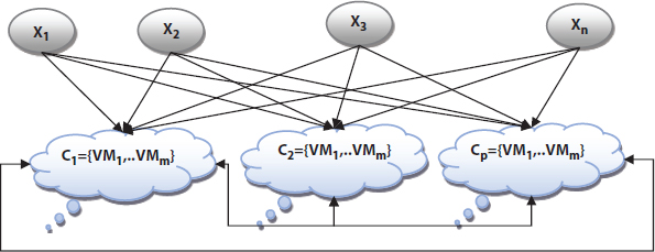
Figure 9.3 Mapping of tasks and virtual machines.
9.3 System Computing Model
It is represented by cloud servers which are communicated in full duplex mode using fast network. Cloud server denoted by SG = {Cs}, where Cs = {C1,C2,…,Cp} is a collection of finite pth cloud servers and each cloud server C1 = {VM1,..,VMm}, C2 = {VM1,..,VMm},…, Cp = {VM1,..,VMm} consists of one or more VMs. Here, cloud server’s VM are heterogeneous platform and they are worked at a distinct speed. The communication time between two tasks Ti and Tj does not consider if they are communicated in same SG; otherwise, it would be considered.
Figure 9.3 showed that mapping of tasks onto corresponding cloud servers.
9.4 Major Objective of Scheduling
The major objective of scheduling of the workflow model is to reduce the overall execution time onto the virtual machine. It is mathematically denoted as follows:
where CCT is completion time of the task.
9.5 Task Computational Attributes for Scheduling
These attributes have major role while allocation of the tasks onto VM and details of seven attributes discussed as below [26]:
- Estimated Computation Time(ECT) [10, 26, 27]
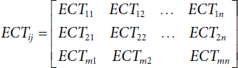
where ECTij for the Xi onto VMj.
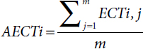
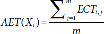
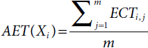
- Average ECT (AECT) [11, 26, 27] of a task Xi is defined as
- Critical Path(CP) [12, 13, 26, 27] is the greatest link from Xentry to Xexit which is as follows:

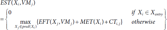
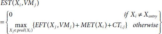
- Earliest Start Time EST [14, 26, 27] which is as follows:
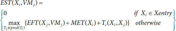
- Minimum Execution Time MET [15, 26, 27] is defined as follows:

- Earliest Finished Time EFT [15, 26, 27] is defined as follows:

- Static Level SL [13, 15, 26, 27]: It can be defined as follows:

9.6 Performance Metrics
Comparison of heuristic algorithms is based on performance metrics which are as follows: scheduling length, scheduling length ratio, speedup and efficiency, resource utilization, and cost.
- i. Scheduling Length [15]: It is an important comparison metrics because it gives the overall execution time of the tasks of a given DAG. Formally, scheduling length is defined as the exit task of a given DAG on available virtual machine will take minimum time, i.e.,

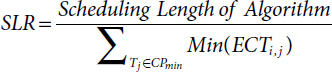
- ii. Scheduling Length Ratio (SLR) [15–17]: It is the ratio of scheduling length and the sum of minimum ECT of critical path (CPmin) task in given DAG, i.e.,
- iii. Speedup [17]: It is defined as the ratio of sum of ECT of all the tasks of given DAG on a VM which will take minimum and scheduling length, i.e.,
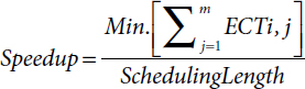
Where m is number of VMs.
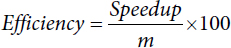
- iv. Efficiency [17]: It is defined as the ratio of speedup and total number of VMs, i.e.,
- v. Resource Utilization [18]: It is important metric for cloud computing which has primary objective is to maximize the resource utilization. It is calculated by average resource utilization (ARU).
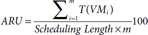
where T(VMi) is time taken by virtual machine i to finish all tasks of given DAG.
- vi. Cost [19]: This metric is defined by following:

where Eij is the running time of Xi on VMj and C (VMj) expensive of VMj per unit time.
9.7 Heuristic Task Scheduling Algorithms
This section will be discussed four well-known heuristic scheduling algorithms such as HEFT [20], CPOP [20], ALAP [12], and PETS [21] in cloud computing environment which is shown in Figure 9.4, and these heuristic algorithms are used as standard algorithms to being comparison with any new algorithms using various performance metrics. All four heuristic algorithms are based on the priority attribute of the tasks and according to their priority; it will be allocated to the machines. Details of the algorithms are presented in subsequent sections.

Figure 9.4 Heuristic algorithms.
9.7.1 Heterogeneous Earliest Finish Time (HEFT) Algorithm
HEFT [20] is a type of list scheduling for heterogeneous platform and it gives good performance with ideal scheduling length. It is worked in two different phase which is as follows:
First Phase: Task Priority
The order of the tasks either ascending or descending is known as the priority for any task. HEFT algorithm uses an upward rank method to compute the task’s priority of the given DAG. This method is also called a b-level (bottom level) attribute. It is denoted by URank and it is based on average execution time and average communication time of the tasks. The computation of the priority of the tasks will start from the exit task and move to upward of the DAG. Formally, it is expressed [20] by:
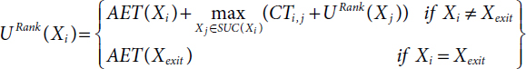
where:
- Xi is the tasks of the given DAG
- Xexit is the last task of the given DAG
- CTi,j is the communication time between the tasks Xi and Xj.
- SUC is a finite set of immediate successor of Xi.
- AET is the average execution time of the task Xi and it can be expressed by:
An Illustrative Example
This section is discussed in detail elaboration of the task priority phase with an example of DAG1 [14, 26, 27] as shown in Figure 9.5 and ECT [14, 26, 27] value of the tasks also given in Table 9.1. The DAG1 has 10 tasks{X1, X2, …, X10} single entry, single exit tasks, and considered two cloud servers CS1 and CS2. The CS1 consists of two virtual machines VM1 and VM2. Similarly, the CS2 consists of one virtual machine VM3.

Figure 9.5 DAG1 model with 10 tasks.
The computation of upward rank (URank) of the tasks of the given DAG1 will be started from the exit task X10 and move toward the upward of the DAG1. The details of the computation [20] are shown in Table 9.2.
Table 9.1 ECT [14, 26, 27] matrix for DAG1 model.
| X1 | X2 | X3 | X4 | X5 | X6 | X7 | X8 | X9 | X10 | |
|---|---|---|---|---|---|---|---|---|---|---|
| CS1 VM1 | 14 | 13 | 11 | 13 | 12 | 13 | 7 | 5 | 18 | 21 |
| CS1 VM2 | 16 | 19 | 13 | 8 | 13 | 16 | 15 | 11 | 12 | 7 |
| CS2 VM3 | 9 | 18 | 19 | 17 | 10 | 9 | 11 | 14 | 20 | 16 |
Table 9.2 Computation of upward rank of the tasks of DAG1.
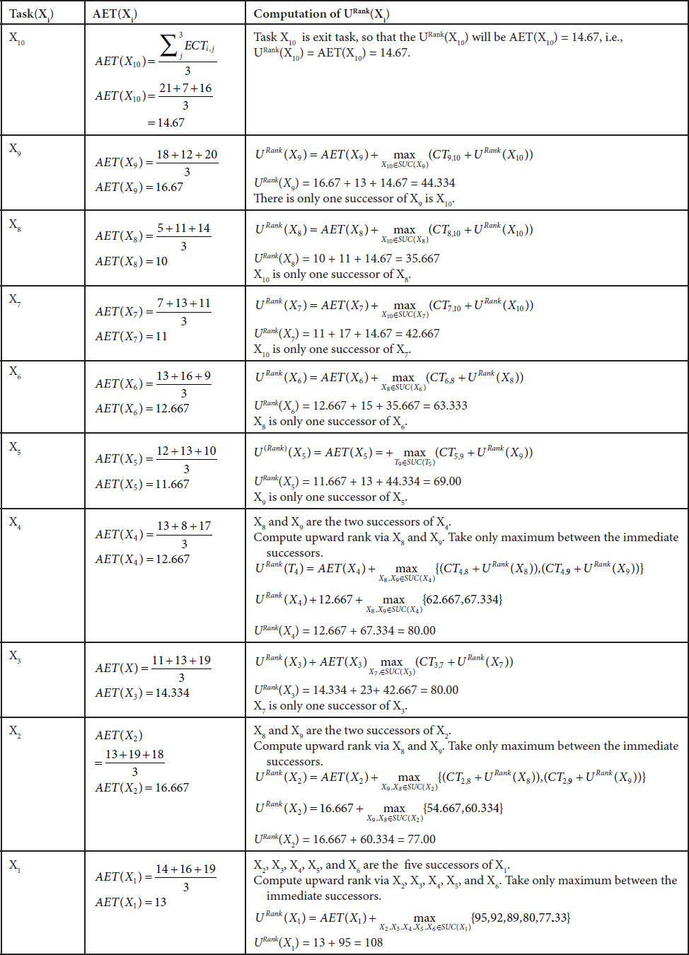
The above table computed the upward rank URanjk of the tasks of the given DAG1 and the URank of all 10 tasks is given below:
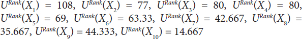
The task priority of the given DAG computed using URank and it would be sorted in decreasing order as per URank value. The sorted order of the tasks is X1, X3, X4, X2, X5, X6, X9, X7, X8, and X10. These tasks are used for allocation in the next phase of the algorithm.
Second Phase: VM Selection
This phase is used to select the tasks as per the priority which is computed in the previous section of task priority phase and these tasks would be scheduled in the suitable virtual machines which gives the optimal finishing time of the tasks.
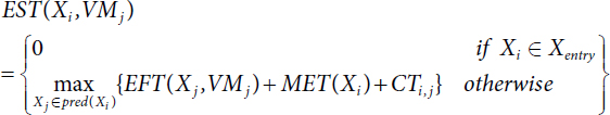
VM selection is based on two important attributes such as EST [14] and EFT [15]. Details of the attributes are given below:
Earliest Start Time EST [26, 27] is defined as follows:
Minimum Execution Time MET [22, 26, 27] is defined as follows:
Earliest Finished Time EFT [26, 27] is defined as follows:
An Illustrative Example
The sorted order of the tasks is X1, X3, X4, X2, X5, X6, X9, X7, X8, and X10. These tasks would be allocated to available virtual machines as per above given attributes and ECT value of the tasks is given in Table 9.1. The precedence constraints of the tasks should be maintained during the allocation of the tasks. Here, consider two cloud servers CS1 and CS2. CS1 consists of two virtual machines VM1 and VM2. CS2 consists of one virtual machine VM3. For this, the Gantt chart [23] is used to represent the tasks allocation onto VM as shown in Figure 9.6. The HEFT algorithm generates 73 units of scheduling length for the given DAG with 10 tasks.

Figure 9.6 Gantt chart for task allocation.
9.7.2 Critical-Path-on-a-Processor (CPOP) Algorithm
CPOP algorithm [20] is another standard heuristic algorithm which is used for comparison with proposed algorithms. This algorithm is also worked in two phases as mentioned in HEFT algorithm such as task priority and VM selection. But finding the priority of the tasks of the given DAG1 is based on summation of two ranks value such as upward rank and downward rank. The tasks of CPOP algorithm are either critical path tasks or non-critical path tasks. The critical path tasks would be allocated on same machine which takes minimum execution time and non critical tasks has no such type of condition for allocation of the tasks on same machine. They would be allocated as per EST and EFT attribute of the tasks. It has a priority queue which maintained as per the value of summation rank value.
First Phase: Task Prioritization
This phase is again classified into three major parts such as prioritization, critical path tasks, and critical path VM. Details of these are as follows:
- a. Prioritization
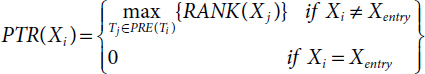
Task prioritization is based on both upward rank URank and downward rank DRank of the tasks of the given DAG1. It can be expressed by [20]:

Where
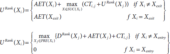
where PRE(Xi) as a finite predecessor set of task Xi.
Formal definition of DRank(Xi) is the greatest distance from Xentry to Xi and avoid the average execution time AET(Xi).
- b. Critical Path Tasks
It has a critical path length |CP| which is the length of the greatest path from Xentry to Xexit of the given DAG1. The value of |CP| is XPriority (Xentry).
This phase also identify the critical path tasks of the given DAG1 which is expressed as follows:
It is designated by CPSET and computed [24] as

This algorithm helps to compute the all tasks on critical path of the given DAG.
- c. Critical Path VM
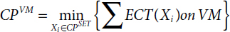
It identifies the virtual machine which takes minimum execution time while computing all critical path tasks CPSET on the same VM, i.e.,
An Illustrative Example
Consider the same example of DAG1 [14, 26] as shown in Figure 9.5 and the ECT [14] value of the tasks that is also given in Table 9.1. The DAG1 [27] consists of 10 tasks, single entry, single exit tasks, and considered two cloud servers CS1 and CS2. The CS1 consists of two virtual machines VM1 and VM2. Similarly, the CS2 consists of one virtual machine VM3. The computation of downward rank (DRank) of the tasks of the given DAG1 will be started from the entry task Tentry and move to downward of the given DAG1. The details of the computation [24] of downward rank (DRank) are shown in Table 9.3 and task priority TPriority computation is shown in Table 9.4.
The value of |CP| is 108 and critical path tasks CPSET would be {X1, X2, X9, X10} and minimum execution time taken by these tasks on VM2 is 54. So, all CPSET tasks are allocated on VM2 during scheduling of the tasks of the given DAG1.
Second Phase: VM Selection
This phase consists of ready queue (RQ) which is initialized by the entry task of the given DAG1. The tasks are removed from RQ one by one, and if removed task Ti belongs to CP SET, then it would schedule onto virtual machine in CPVM otherwise it would schedule onto a virtual machine which takes minimum EFT. All successor tasks Tj of Ti would be inserted into RQ as per the value of TPriority. Precedence constraint always should be maintained during the allocation onto a virtual machine otherwise give the chance to the next low priority task.
An Illustrative Example
The order of the task as per CPOP algorithm is X1, X2, X3, X7, X4, X5, X6, X8, and X10 of the given DAG1 in Figure 9.5. The ECT value of the tasks is given in Table 9.1. Here, consider two cloud servers CS1 and CS2. CS1 consists of two virtual machines VM1 and VM2. CS2 consists of one virtual machine VM3. For this, the Gantt chart [23] is used to represent the tasks allocation onto VMs as shown in Figure 9.7. The CPOP algorithm generates 86 units of scheduling length for the given DAG1 with 10 tasks.
Table 9.3 Computation of downward rank of the tasks of DAG1.
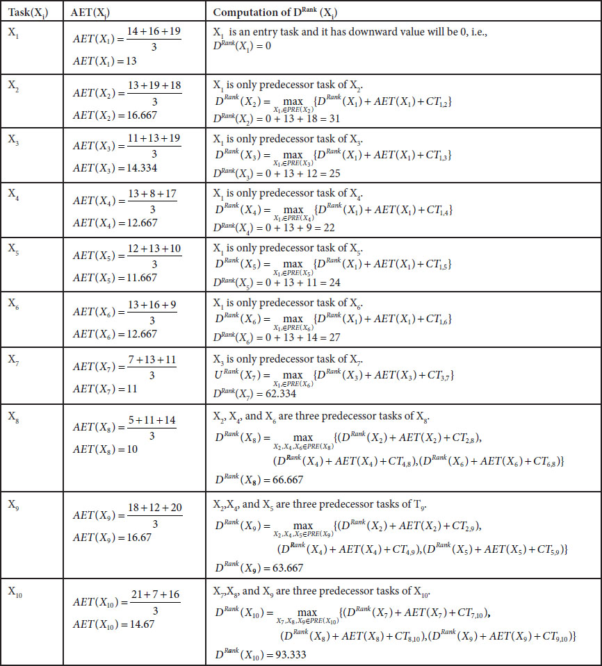
Table 9.4 Computation of task priority TPriority [20] of the tasks of DAG1.
| Task(Xi) | URank(Xi) | DRank(Xi) | TPriority(Xi) = URank(Xi) + DRank(Xi) |
|---|---|---|---|
| X1 | 108 | 0 | 108 |
| X2 | 77 | 31 | 108 |
| X3 | 80 | 25 | 105 |
| X4 | 80 | 22 | 102 |
| X5 | 69 | 24 | 93 |
| X6 | 63.33 | 27 | 90.33 |
| X7 | 42.66 | 62.33 | 105 |
| X8 | 35.66 | 66.66 | 102.33 |
| X9 | 44.33 | 63.66 | 108 |
| X10 | 14.66 | 93.33 | 108 |

Figure 9.7 Gantt chart for task allocation.
9.7.3 As Late As Possible (ALAP) Algorithm
ALAP [12] is a scheduling algorithm worked on both heterogeneous and homogeneous platforms. There are two phases of this algorithm such as task prioritization and VM selection.
Task Prioritization Phase
The task prioritization phase is computed as the difference between critical path CPath and upward rank URank of the tasks Xi of the given DAG1. It can be expressed as
CPath is the length of path from entry task to exit task where length is the longest. This attribute is expressed [13] as follows:
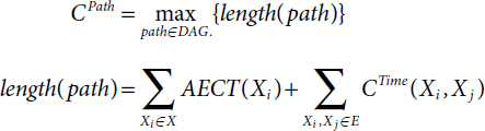
where
- AECT(Xi)[20] is the Average Estimated Computation Time of task Xi and it can be computed as
 , m is total number of VMs.
- CTime (Xi, Xi) is the Communication time between the tasks Xi and Xj.
- E is a finite set of edges of DAG.
- X is a finite set of tasks of DAG.
URank(Xi) is the longest path from Xi to Xexit tasks and it includes the execution time of Ti. Upward Rank is also called Bottom Level (B-Level). URank(Xi) is expressed as follows:
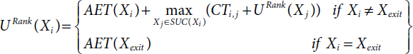
where:
- Xi is the tasks of the given DAG
- Xexit is the last task of the given DAG
- CTi,j is the Communication Time Between the tasks Xi and Xj.
- SUC is a finite set of immediate successor of Xi.
- AET is the Average Execution Time of the task Xi and it can be expressed by:
VM Selection Phase
After computing the priority of the tasks of the given DAG1, it would be sorted for scheduling in cloud server’s virtual machines.
This phase decides the selection of a particular virtual machine as per minimum EST and EFT attributes. Details of EST and EFT attributes are as below:
Earliest Start Time EST [26, 27] as follows:
EST(Xi,VMj)
Minimum Execution Time MET [22, 26, 27] as follows:
Earliest Finished Time EFT [26, 27] as follows:
An Illustrative Example
Consider a DAG1 [14, 26, 27] as shown in Figure 9.5 and ECT [14, 26, 27] value of the tasks as also given in Table 9.1. This DAG1 has 10 tasks, single entry, single exit tasks and considered two cloud servers CS1 and CS2. CS1 consists of two virtual machines VM1 and VM2. Similarly, CS2 consists of one virtual machine VM3.
Critical path of the tasks is shown in Figure 9.8 as the red bold line and the value of CPath is 108. Details computation of the task priority TPriority of the task Xi of the given DAG1 are shown in Table 9.5.
The sorted the TPriority tasks Xi in ascending order such as X1, X3, X4, X2,X5, X6, X9, X7, X8, and X10 of the given DAG in Figure 9.5. ECT value of the tasks is given in Table 9.1, which is used while allocating these onto the virtual machines. Here, consider two cloud servers CS1 and CS2. CS1 consists of two virtual machines VM1 and VM2. CS2 consists of one virtual machine VM3. For this, Gantt chart [23] is used to represent the tasks allocation onto VM as shown in Figure 9.9. The ALAP algorithm generates 73 units of scheduling length for the given DAG with 10 tasks.
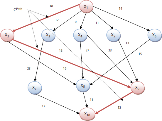
Figure 9.8 DAG model with 10 tasks.
Table 9.5 Computation of the task priority TPriority.
| Task(Xi) | URank(Xi) | TPriority(Xi) = CPath − URank(Xi) |
|---|---|---|
| X1 | 108 | 0 |
| X2 | 77 | 31 |
| X3 | 80 | 28 |
| X4 | 80 | 28 |
| X5 | 69 | 39 |
| X6 | 63.33 | 44.667 |
| X7 | 42.66 | 65.333 |
| X8 | 35.66 | 72.333 |
| X9 | 44.33 | 63.667 |
| X10 | 14.66 | 93.333 |

Figure 9.9 Gantt chart for task allocation.
9.7.4 Performance Effective Task Scheduling (PETS) Algorithm
PETS [21] algorithm is worked in three phases such as sorting of task level, prioritization of task, and VM selection.
First Phase: Sorting of Task Level
This phase is used to find levels with their respective tasks and it is traversed from top to bottom of the given DAG. Each level consists of multiple tasks which are independent and these tasks would be sorted and grouped as appeared in their level. For example, task level sorting of the given DAG as shown in Figure 9.5 is divided into four levels. Level1 consists of entry task X1, Level2 consists of intermediate tasks X2, X3, X4, X5, X6, and so on for the other two levels. Sorting of task level is shown in Table 9.6.
Second Phase: Prioritization of Task
This phase is used to compute the priority and assign to the tasks of the given DAG1. There are three attributes [21] that are designed to compute the priority of the tasks and the attributes are average execution time (AET), data communication time (DCT), and predecessor task rank (PTR). Details of these attributes are given below:
AET of the task Ti is defined as by  . For example, the AET of the tasks of the given DAG shown in Figure 9.5 and using the ECT value of the DAG in Table 9.1 Details of AET computation are shown in Table 9.7.
Table 9.6 Sorting of task level.
| Level | Task Group |
|---|---|
| 1 | {X1} |
| 2 | {X2,X3,X4,X5,X6} |
| 3 | {X7,X8,X9} |
| 4 | {X10} |
DCT of the task Xi is defined as the summation of communication time of immediate successor tasks Xj of Xi at each level. It can be expressed [21] as
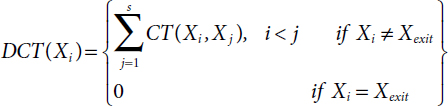
where s is the total number of tasks in next level.
An example of DCT of the tasks of DAG1 is given in Figure 9.5. X1 has five successor tasks X2, X3, X4, X5, and X6 and the summation of the communication time CT between X1 and all its successor tasks is 64. Similarly, DCT computation for rest tasks at each level is shown in Table 9.8.
PTR of the tasks Xi is the greatest rank of immediate predecessors Xj of Xi, and it can be computed[21] as follows:
where PRE is immediate predecessor tasks Xj of Xi.
RANK of task Xi is computed based on AET, DCT, and PRT of the task. It is computed as follows:
Table 9.7 AET computation.
| Task(Xi) | X1 | X2 | X3 | X4 | X5 | X6 | X7 | X8 | X9 | X10 |
|---|---|---|---|---|---|---|---|---|---|---|
 |
13 | 16.67 | 14.34 | 12.67 | 11.67 | 12.67 | 11 | 10 | 16.67 | 14.67 |
Table 9.8 DCT computation.
| Task(Xi) | X1 | X2 | X3 | X4 | X5 | T6 | X7 | X8 | X9 | X10 |
|---|---|---|---|---|---|---|---|---|---|---|
| DCT(Xi) | 64 | 35 | 23 | 50 | 13 | 15 | 17 | 11 | 13 | 0 |
Table 9.9 Computation of PTR, RANK, and Priority.
| Level | Task(Xi) | DCT(Xi) | AET(Xi) | PTR(Xi) | RANK(Xi) | Priority |
|---|---|---|---|---|---|---|
| 1 | X1 | 64 | 13 | 0 | 77 | 1 |
| 2 | X2 | 35 | 16.67 | 77 | 129 | 2 |
| X3 | 23 | 14.34 | 77 | 115 | 3 | |
| X4 | 50 | 12.67 | 77 | 140 | 1 | |
| X5 | 13 | 11.67 | 77 | 102 | 5 | |
| X6 | 15 | 12.67 | 77 | 105 | 4 | |
| 3 | X7 | 17 | 11 | 115 | 143 | 3 |
| X8 | 11 | 10 | 140 | 161 | 2 | |
| X9 | 13 | 16.67 | 140 | 170 | 1 | |
| 4 | X10 | 0 | 14.67 | 170 | 185 | 1 |
The priority of the tasks at each level is decided by its rank value. If a task has the greatest rank in their level, then its priority will also be the highest among the tasks. Details of PRT, RANK, and Priority of the tasks are shown in Table 9.9 of the given DAG1 in Figure 9.5.
Third Phase: VM Selection
After the computed the priority of the tasks of the given DAG1, it would be sorted for scheduling in cloud server’s virtual machines. This phase decides the selection of a particular virtual machine as per minimum EST and EFT attributes. Details of EST and EFT attributes as below:
Earliest Start Time EST [26, 27] is defined as follows:
Minimum Execution Time MET [22, 26, 27] is defined as follows:
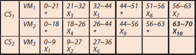
Figure 9.10 Gantt chart for task allocation.
Earliest Finished Time EFT [26, 27] is defined as follows:
Illustrative Example
The order of the tasks as per the priority are X1, X4, X2, X3, X6, X5, X9, X8, X7, and X10 of the DAG1 in Figure 9.5. The ECT value of the tasks is given in Table 9.1 which is used while allocating these onto the virtual machines. Here, consider two cloud servers CS1 and CS2. CS1 consists of two virtual machines VM1 and VM2. CS2 consists of one virtual machine VM3. For this, Gantt chart [23] is used to represent the tasks allocation onto VM as shown in Figure 9.10. The PETS algorithm generates 70 units of scheduling length for the give DAG with 10 tasks.
9.8 Performance Analysis and Results
The analysis of four heuristics algorithms such as HEFT, CPOP, ALAP, and PETS has done using two directed graphs DAG1 and DAG2 as shown in Figures 9.5 and 9.11. This paper discussed six performance metrics in the previous section and they are used as comparison purposed among the four heuristics algorithms. Scheduling length of all heuristic algorithms is found for DAG1 at the starting of the chapter according the algorithms. Other performance metrics such as efficiency, speedup, SLR, and resource utilization are based on scheduling length. The cost table for DAG1 is shown in Table 9.10 [25].
Similarly, the computation of scheduling length of all four heuristic algorithms is computed for DAG2, and value of rest metrics is also shown in table. The ECT table is shown in Tables 9.1 and 9.11 for both DAG1 and DAG2 and cost table of DAG2 is shown in Table 9.12.
The value of all six performance metrics is shown in Table 9.13 [25]. The graphical representation of all performance metrics for four heuristic algorithms is shown in Figures 9.12 to 9.17.
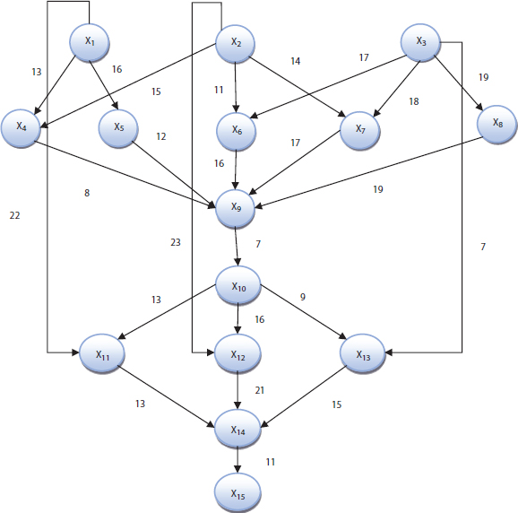
Figure 9.11 DAG2 model with 15 tasks.
Table 9.10 VM rate for DAG1.
| Virtual Machine (VM) | VM1 | VM2 | VM3 |
|---|---|---|---|
| Cost/Unit Time | 1.71 | 1.63 | 1.21 |
Table 9.11 ECT [15, 27] matrix for DAG2 model.
| X1 | X2 | X3 | X4 | X5 | X6 | X7 | X8 | X9 | X10 | X11 | X12 | X13 | X14 | X15 | |
|---|---|---|---|---|---|---|---|---|---|---|---|---|---|---|---|
| CS1 VM1 | 17 | 14 | 19 | 13 | 19 | 13 | 15 | 19 | 13 | 19 | 13 | 15 | 18 | 20 | 11 |
| CS1 VM2 | 14 | 17 | 17 | 20 | 20 | 18 | 15 | 20 | 17 | 15 | 22 | 21 | 17 | 18 | 18 |
| CS2 VM3 | 13 | 14 | 16 | 13 | 21 | 13 | 13 | 13 | 13 | 16 | 14 | 22 | 16 | 13 | 21 |
| CS2 VM4 | 22 | 16 | 12 | 14 | 15 | 18 | 14 | 18 | 19 | 13 | 12 | 14 | 14 | 16 | 17 |
Table 9.12 VM cost for DAG2.
| Virtual Machine(VM) | VM1 | VM2 | VM3 | VM4 |
|---|---|---|---|---|
| Cost/Unit Time | 1.72 | 1.52 | 1.69 | 1.65 |
Table 9.13 Comparison results.
| DAG Models | Scheduling Algorithms | Performance Metrics Results | |||||
|---|---|---|---|---|---|---|---|
| Scheduling Length | Speedup | Efficiency (%) | SLR | Resource Utilization (%) | Cost/Unit Time | ||
| DAG1 | HEFT | 73 | 1.74 | 58.00 | 1.78 | 77.12 | 258.65 |
| CPOP | 86 | 1.48 | 49.22 | 2.09 | 77.51 | 301.12 | |
| ALAP | 73 | 1.74 | 58.00 | 1.78 | 77.16 | 258.65 | |
| PETS | 70 | 1.81 | 60.33 | 1.71 | 80.47 | 265.39 | |
| DAG2 | HEFT | 152 | 1.52 | 38.00 | 1.71 | 69.73 | 702.75 |
| CPOP | 164 | 1.41 | 35.25 | 1.84 | 64.93 | 694.92 | |
| ALAP | 155 | 1.49 | 37.25 | 1.74 | 72.74 | 751.53 | |
| PETS | 152 | 1.52 | 38.00 | 1.71 | 65.13 | 666.43 | |
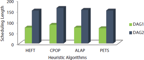
Figure 9.12 Scheduling length.
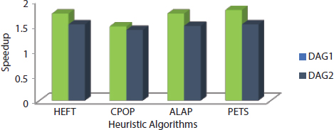
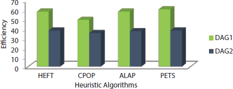
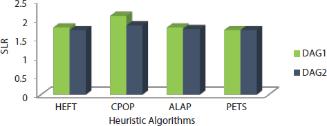
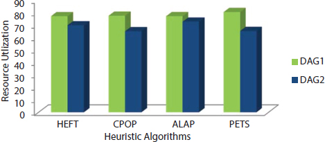

Figure 9.17 Cost.
9.9 Conclusion
This chapter has discussed four heuristic algorithms such as HEFT, CPOP, ALAP, and PETS. These algorithms are used as standard algorithms for comparison purpose with any new proposed algorithms. All four heuristic algorithms are studied in detail and illustrated with help of DAG1 and DAG2 with 10 and 15 tasks, respectively. These algorithms are used various attribute to find the priority of the tasks of the given DAG. The comparative studied of the heuristic algorithms has done based on six performance metrics for both DAG with 10 and 15 tasks, respectively.
References
1. Hashizume, K., Rosado, D.G., Fernández-Medina, E., Fernandez, E.B., An analysis of Security Issues for Cloud Computing. J. Internet Serv. Appl., 4, 1, 5, 1–13, 2013.
2. Pachghare, V.K., Cloud Computing, PHI, Delhi India, 2016.
3. Zhao, G., Liu, J., Tang, Y., Sun, W., Zhang, F., Ye, X., Tang, N., Cloud Computing: A Statistics Aspect of Users. First International Conference on Cloud Computing (CloudCom), Beijing, China, Springer Berlin, Heidelberg, pp. 347–358, 2009.
4. Zhang, S., Zhang, S., Chen, X., Huo, X., Cloud Computing Research and Development Trend. Second International Conference on Future Networks (ICFN’10), Sanya, Hainan, China, IEEE Computer Society, Washington, DC, USA, pp. 93–97, 2010.
5. Gary, M.R. and Johnson, D.S., Computer and Intractability: A Guide to the theory of NP Completeness, W.H freeman, San Francisco CA, 1989.
6. Yadav, A.K. and Mandoria, H.L., Study of Task Scheduling Algorithms in the Cloud Computing Environment: A Review. Int. J. Comput. Sci. Inf. Technol., 8, 4, 462–468, 2017.
7. Kaur, R. and Kaur, R., Multiprocessor Scheduling using Task Duplication Based Scheduling Algorithms: A Review Paper. Int. J. Appl. Innov. Eng. Manage., 2, 4, 311–317, April, 2013.
8. Chung, Y.-C. and Ranka, S., Applications and Performance Analysis of a Compile-Time Optimization Approach for List Scheduling Algorithms on Distributed Memory Multiprocessors. Supercomputing ‘92:Proceedings of the 1992 ACM/IEEE Conference on Supercomputing, Minneapolis, MN, USA, pp. 512–521, 1992.
9. Srinivas, G.N. and Musicus, B.R., Generalized Multiprocessor Scheduling for Directed Acyclic Graphs, in: Third Annual ACM Symposium on Parallel Algorithms and Architectures, pp. 237–246, 1994.
10. Zanywayingoma, F.N. and Yang, Y., Effective Task Scheduling and Dynamic Resource Optimization based on Heuristic Algorithms in Cloud Computing Environment. KSII Trans. Internet Inf. Syst., 11, 12, 5780–5802, 2017.
11. Haidri, R.A., Katti, C.P., Saxena, P.C., Cost Effective Deadline Aware Scheduling Strategy For Workflow Applications on Virtual Machines in Cloud Computing. J. King Saud Univ.- Comp. Info. Sci., 32, 6, July 2020.
12. Kwok, Y.-K. and Ahmad, I., Static Scheduling Algorithms for Allocating Directed Task Graphs to Multiprocessors. ACM Comput. Surv., 31, 4, 1–88, December, 1999.
13. Sinnen, O., Task Scheduling for Parallel Systems, Wiley Interscience Pulication, Hoboken, New Jersey, 2007.
14. Kumar, M.S., Gupta, I., Jana, P.K., Delay-based workflow scheduling for cost optimization in heterogeneous cloud system. Tenth International Conference on Contemporary Computing (IC3), Noida, pp. 1–6, 2017.
15. Gupta, I., Kumar, M.S., Jana, P.K., Efficient Workflow Scheduling Algorithm for Cloud Computing System: A Dynamic Priority-Based Approach. Arab. J. Sci. Eng., 43, 12, 7945–7960, 2018.
16. Hwang, K., Advanced Computer Architecture: Parallelism, Scalability, Programmability, TMH Publishing Company, New Delhi, 2005.
17. Akbar, M.F., Munir, E.U., Rafique, M.M., Malik, Z., Khan, S.U., Yang, L.T., List-Based Task Scheduling for Cloud Computing. IEEE International Conference on Internet of Things (iThings) and IEEE Green Computing and Communications (GreenCom) and IEEE Cyber, Physical and Social Computing (CPSCom) and IEEE Smart Data (SmartData), Chengdu, pp. 652–659, 2016.
18. Kalra, M. and Singh, S., A Review of Metaheuristic Scheduling Techniques in Cloud Computing. Egypt. Inform. J., 16, 3, 275–295, 2015.
19. Benalla, H., Ben Alla, S., Touhafi, A., Ezzati, A., A Novel Task Scheduling Approach Based On Dynamic Queues And Hybrid Meta-Heuristic Algorithms for Cloud Computing Environment. Cluster Comput., 21, 4, 1797–1820, 2018.
20. Topcuoglu, H., Hariri, S., Wu, M.-Y., Performance-effective and low-complexity task scheduling for heterogeneous computing. IEEE Trans. Parallel Distrib. Syst., 13, 3, 260–274, March, 2002.
21. Ilavarasan, E. and Thambidurai, P., Low Complexity Performance Effective Task Scheduling Algorithm For Heterogeneous Computing Environments. J. Comput. Sci., 3, 2, 94–103, 2007.
22. Xavier, S. and Jeno Lovesum, S.P., A Survey of Various Workflow Scheduling Algorithms in Cloud Environment. Int. J. Sci. Res. Publ., 3, 2, 1–3, February, 2013.
24. Prajapati, K.D., Raval, P., Karamta, M., Potdar, M.B., Comparison of Virtual Machine Scheduling Algorithms in Cloud Computing. Int. J. Comput. Appl., 83, 15, 12–14, December, 2013.
25. Rajak, N. and Shukla, D., Performance Analysis of Workflow Scheduling Algorithm in Cloud Computing Environment using Priority Attribute. Int. J. Adv. Sci. Technol., 28, 16, 1810–1831, 2019.
26. Rajak, N. and Shukla, D., An Efficient Task Scheduling Strategy for DAG in Cloud Computing Environment, in: Ambient Communications and Computer Systems. Advances in Intelligent Systems and Computing, vol. 1097, Y.C. Hu, S. Tiwari, M. Trivedi, K. Mishra (Eds.), Springer, Singapore, 2020.
27. Rajak, N. and Shukla, D., A Novel Approach of Task Scheduling in Cloud Computing Environment, in: Social Networking and Computational Intelligence. Lecture Notes in Networks and Systems, vol. 100, R. Shukla, J. Agrawal, S. Sharma, N. Chaudhari, K. Shukla (Eds.), Springer, Singapore, 2020.
- *Corresponding author: [email protected]