
Chapter 14
Crunching Numbers (and Data) with Excel
IN THIS CHAPTER
![]() Selecting a template
Selecting a template
![]() Entering, formatting, and editing data
Entering, formatting, and editing data
![]() Using copy-and-paste for formatting
Using copy-and-paste for formatting
![]() Using AutoFill
Using AutoFill
![]() Checking for errors in your calculations
Checking for errors in your calculations
![]() Filtering and sorting data
Filtering and sorting data
![]() Using Find and Replace to help with editing your spreadsheets
Using Find and Replace to help with editing your spreadsheets
Excel’s power as a spreadsheet derives from the flexibility it provides you in entering, formatting, deriving, analyzing, and presenting your data. Producing a bare grid of unformatted, manually entered text and numeric cells would make even the most compulsive Bob Cratchit exhausted, bored, and cross-eyed. Excel’s powerful formula creation tools help you quickly and easily calculate results from your data, and Excel’s formatting capabilities let you almost effortlessly draw attention to important data and results and, when desired, make supporting data fade into the background.
In this chapter, you find out how to use Excel’s timesaving and effort-minimizing features to avoid exhaustion, boredom, and ocular fatigue.
Working with Templates
Traditionally, a spreadsheet (including Excel’s) starts as an empty grid filled with identically sized cells. Although such a blank canvas offers incredible flexibility, many users instead consider it incredibly intimidating. Excel’s templates let you avoid that vast expanse of emptiness by providing preconfigured and preformatted worksheets for a wide variety of common tasks that are just waiting for you to input your data into the indicated cells.
Just as it does for Word, PowerPoint, and Outlook, Microsoft Office offers Excel templates — these local templates are installed as part of Office and you don’t have to be online to access them. Just as Word templates provide a starting point when you want to create a specific type of word processing document (for example, a newsletter or a flyer), Excel templates give you a head start and framework for creating specific spreadsheet documents or performing common spreadsheet tasks (such as managing a household budget or computing and structuring a home mortgage).
And don’t forget that internet thing. Excel also offers online templates contributed by other Excel users. You can find a huge number of templates covering all sorts of common spreadsheet tasks. You can also find specific templates for movie collections, billing statements, timesheets, and more. Heck, you can find templates for purposes you’d never expect. Of course, you need an active internet connection to load these templates.
The following sections provide more details about finding and taking advantage of Excel templates.
Choosing a local template
The Workbook gallery collects all Microsoft-supplied local Excel templates and makes them available in a single location.
To create a document from a local Workbook gallery template, follow these steps:
- Choose File ⇒ New from Template or press Shift+⌘ +P.
-
From the list on the left, click New.
The local templates fill the large pane on the right, as shown in Figure 14-1.
- Select the thumbnail representation of the template you want and click Create. (Alternatively, double-click the template’s thumbnail.)
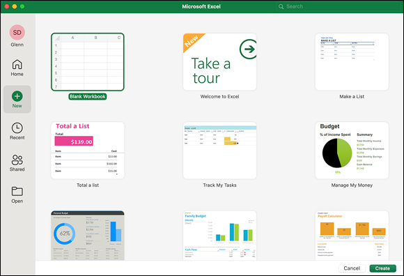
FIGURE 14-1: Excel comes loaded with several local templates to choose from.
Excel opens a new document based on the template you selected, and that’s all there is to it. Now all you have to do is make the template your own document by entering data into the cells.
 Click the Recent icon on the left of the Workbook gallery to display the Recent tab. There you'll find workbooks you’ve created, opened, or modified today, yesterday, or within the past week or past month.
Working with online templates
Online templates are maintained by Microsoft on its templates website, https://templates.office.com. You may be able to locate many of the internet-supplied templates by clicking the search field in the upper-right corner of the Workbook gallery and typing a name or category. Figure 14-2 shows a search for templates related to cards.
Microsoft continually changes and updates template categories and subcategories online, but you’re always likely to find our favorite categories:
- Budgets includes templates for tracking and managing your personal income and expenses as well as your business budget.
- Invoices includes templates containing columns and formulas common to tracking and managing invoices.
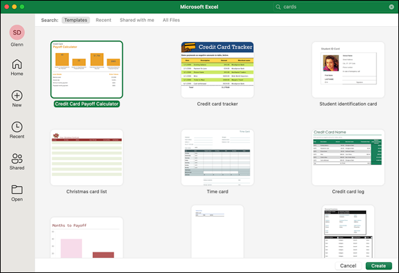
FIGURE 14-2: Microsoft provides dozens of templates that you can search for.
- Lists, as its name implies, includes numerous preformatted templates set to manage various common list types, including team rosters, chore charts, and grocery lists. Be sure to check out what’s available in this category; you’re bound to find at least one that comes in handy for helping to manage your everyday affairs.
- Reports includes all sorts of templates designed to generate common reports.
You can find and download more templates from Microsoft by visiting https://templates.office.com. You’ll find templates for just about any type of spreadsheet you can imagine, and then some.
Entering, Formatting, and Editing Data in Cells
Several decades ago, when Dan Bricklin’s VisiCalc swept personal computers from the domain of hobbyists (read “nerds”) into the realm of business, you selected a cell and then entered the spreadsheet data for that cell in a data entry box. This paradigm remains available to traditionalists by way of the traditional data-entry mechanism known as the Excel formula bar (see Figure 14-3). You specify the cell in the Name box on the left and then enter the data or formula in the Formula box on the right.
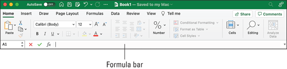
FIGURE 14-3: The formula bar.
A modern graphical user interface (GUI), such as the one to which we Mac users are accustomed, begs us to enter our data directly into the cells where it belongs, and Excel obliges. Just click a cell (or navigate to it using your keyboard’s cursor keys or by typing in the Name box in the formula bar) and start typing. Then move to the next cell and enter its data.
The cell data you enter or edit appears in the formula bar, but any formatting you apply via the Home tab on the ribbon or the Format menu appears only in the cell, as shown in Figure 14-4.
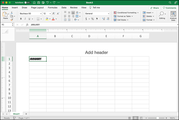
FIGURE 14-4: Formatting isn’t reflected in the formula bar.
All the usual editing techniques are available when working with a cell’s contents. You can select all or part of the data and apply formatting via the ribbon; replace the selection by typing or pasting, and position the insertion point and then type or paste new data, for example.
Copying and Pasting Data (and Formatting) between Cells
We expect any Mac app that allows data entry to support copying (and cutting) and pasting data as well. Excel doesn’t disappoint in that respect, but adds a few small wrinkles. For example, copying from one cell and then pasting in another brings the data, but you may not want to retain its original formatting. If you want to select which formatting is retained, right-click the destination cell, choose Paste Special from the contextual menu, and then select Paste Special again. You’re presented with the dialog shown in Figure 14-5.
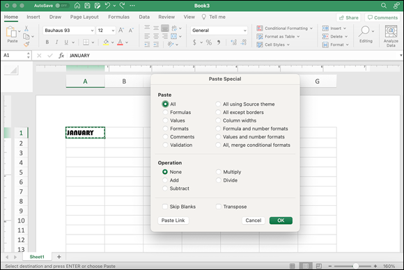
FIGURE 14-5: Paste Special lets you paste values, formulas, formatting, and more.
Clicking the Paste button on the ribbon’s Home tab isn’t quite the same as choosing Edit ⇒ Paste. Instead, as shown in Figure 14-6, Excel pastes the data and displays a small paste options icon with a drop-down menu attached (Microsoft calls them smart buttons), in which you can choose to retain the formatting of the source being copied or to apply destination formatting (that is, any formatting you’ve already applied to the destination cell).
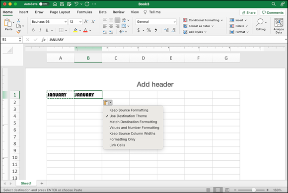
FIGURE 14-6: Using the toolbar’s paste options button gives you a formatting choice.
You might also be a little disconcerted the first time you choose Edit ⇒ Cut. Rather than make the data disappear, as this command does in most Office apps, it creates a dotted outline border on the selected cell. When you select another cell and paste, the data and the outline disappear.
You can make the outline stop shimmering without losing the selection by pressing Esc.
Finally, you can use the format icon (paintbrush) on the left side of the ribbon’s Home tab to copy only a cell’s formatting and apply it to one or more other cells. Follow these steps:
- Select a cell containing the formatting you want to use.
- Click the paintbrush icon (format) on the Home tab of the ribbon.
- Drag across the cell (or cells) to which you want to apply this formatting.
You can lock the Format tool by double-clicking. Locking it lets you apply the selected formatting to multiple noncontiguous cells or ranges of cells. Clicking the locked Format tool unlocks it.
AutoFilling Cells
Spreadsheet users commonly want to fill a group of cells (rows or columns) with data. Sometimes, you need to work with a series of numbers (for example, 1–30) or common text labels (such as days of the week or months of the year), and sometimes, you need to use a repeated value (such as a default zip code).
To AutoFill a set of cells, follow these steps:
-
Hover the cursor over the lower-right corner of the cell containing the initial value or the value to be repeated.
This action displays the fill handle, as shown on the left in Figure 14-7.
-
Drag down (or across) a group of cells, as shown on the right in Figure 14-7.
Your values fill the cells you’re dragging over.
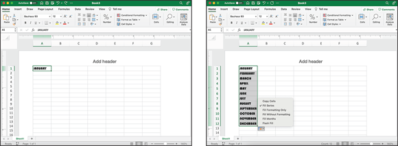
FIGURE 14-7: Get a fill handle (left) and drag through the cells you want to fill (right).
Clicking the AutoFill smart button’s drop-down arrow presents fill choices. The default is Fill Series.
An alternative to dragging with the mouse is to select a group of cells, type the information you want in one of them, and then press Control+Return to fill all the selected cells with that information.
If you don’t want to have the smart button appear when you drag the fill handle, choose Excel ⇒ Preferences, click the Edit button, and deselect the Show Insert Options check box. Click OK to accept any preference changes you made.
Understanding Formulas and Functions
If all Excel allowed you to do was enter and format literal values in the sheet’s cells, you would have a useful electronic implementation of a ledger book, but you would be missing out on a spreadsheet’s real power — the capability to automatically calculate values in one cell based on the values in one or more other cells. The calculation that an Excel spreadsheet can perform is as basic as showing the sum or difference between two values or as advanced as working with a complex formula involving a variety of common statistical, trigonometric, financial, or date conversion functions. For example, in a Wedding Budget template, cell B9 might contain a formula (=B6-B8), telling Excel to calculate the available budget for your wedding by subtracting the actual expenses incurred to date from the total budget amount you’ve allotted.
Excel comes with hundreds of built-in functions, divided into categories. You can find a lengthy list, including descriptions of the functions, in Excel’s Help system: Go to Help ⇒ Excel Help, type Excel functions, and then click either Excel functions (by category) or Excel functions (alphabetical) to explore them.
Many functions are general purpose, such as SUM, which totals the values in the referenced cells. Others are of interest only to users in specific fields. The ATANH function (which returns a value’s inverse hyperbolic tangent, if that means anything to you!) is useful to mathematicians and engineers, and DDB (which returns asset depreciation based on the double-declining balance method) probably doesn’t do much for you unless you’re an accountant.
Creating a formula
When creating a formula, the first character in the formula must be the equal sign (=), which tells Excel that a formula follows, not text or numeric data.
Functions and formulas reference cells by name: for example, A1 or F10. You can also use a shorthand method to indicate a contiguous range of cells. For example, A1:A4 tells Excel that cells A1, A2, A3, and A4 are all arguments, and A1:B3 specifies that A1, B1, A2, B2, A3, and B3 are arguments. As you can see, using this shorthand for a cell range can significantly cut down on your typing time and make your intent clear. Furthermore, you can have multiple ranges in your argument list. (For example, A1:B3, D5:F7, A10:F10 specifies that all 21 cells referenced in the three ranges are the arguments to your function.) When referencing cells, you can use two forms of address — relative and absolute — to make a large difference. Check out the nearby “Absolute versus relative references” sidebar for the skinny on this important concept.
Keeping track of Excel formulas with Formula Builder
With the multitude of Excel built-in functions, many sporting somewhat cryptic names and taking multiple arguments, remembering just which function you need at any given time can be a daunting task. Excel eases the pain with Formula Builder. You can display the Formula Builder pane (shown in Figure 14-8) by choosing Formula Builder from the View menu. Also, you can click the More Help on This Function link in the Description box to call up Excel Help and display a full description of the selected function.
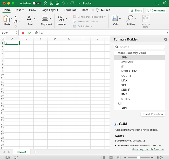
FIGURE 14-8: Formula Builder makes finding and using Excel’s built-in functions easy.
Selecting a function in the list gives you a brief description of it, as shown in Figure 14-8.
Formula Builder’s window (see Figure 14-9) is ready for you to start plugging in argument values as Excel starts building your formula in the selected cell.
Another Excel feature that aids you in constructing formulas is Formula AutoComplete. Formula AutoComplete kicks in when you start typing a function’s name in a cell. A list of matching names appears, and you can select the one you want from the list to complete the name (by either clicking or selecting it with the arrow keys and then pressing Return or Enter). For example, if you type =av (you must type the equal sign first to engage Formula AutoComplete), as shown in Figure 14-10, Excel displays all functions whose names start with those two letters. After you select the function you want, the cursor is positioned in the function’s argument list, awaiting your input.
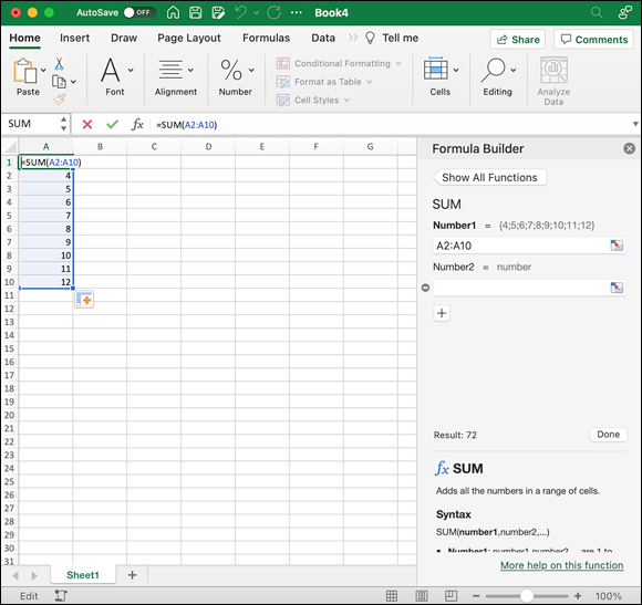
FIGURE 14-9: Excel builds your formula as you fill in the blanks in Formula Builder.
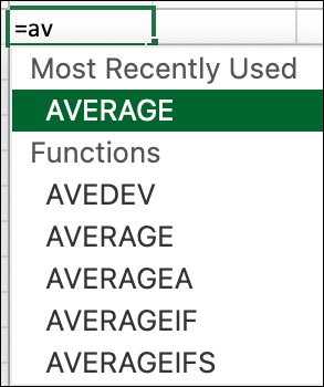
FIGURE 14-10: Formula AutoComplete helps you cut down on typing by narrowing the list of available functions as you type.
If AutoComplete isn’t working for you, you need to turn on the feature:
- Choose Excel ⇒ Preferences from the menu, or press ⌘ +, (comma).
- In the Preferences dialog, click AutoComplete in the Formulas and Lists section.
- Select the Show AutoComplete Options for Functions and Named Ranges check box, as we did in Figure 14-11.

FIGURE 14-11: Enable AutoComplete in Excel’s Preferences dialog.
Using the Error Checking Feature
In Excel (or any other data presentation tool), the results can be only as accurate as the underlying data. Excel can’t read your mind. If you create a formula that subtracts where it should add, your results will be erroneous and you can easily take incorrect action based on those erroneous results. Unfortunately, Excel can’t save you from that class of error, any more than it can prevent you from entering 12 when you meant to enter 1.2 (assuming that both values are permissible for that cell). However, Excel can warn about some types of errors. The values that Excel checks are controlled in the Excel Preferences Error Checking pane, shown in Figure 14-12. To open this pane, choose Excel ⇒ Preferences and then click the Error Checking icon.
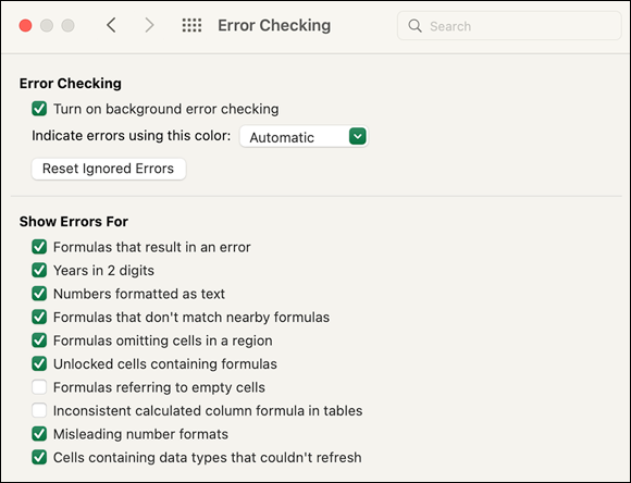
FIGURE 14-12: Control the types of errors Excel checks for in the Error Checking pane.
When Excel spots an error, it displays a small triangle in the cell’s upper-left corner. If you click the offending cell, a smart button containing a caution icon (an exclamation point in a yellow diamond) appears. Click the smart button’s drop-down arrow and choose an option to help you resolve the issue. After you’ve corrected the problem, Excel removes the error code and the indicator.
For some people, those little menu triangles are difficult to see and, in a sheet with a lot of text, the error codes don’t necessarily stand out. Excel provides the Error Checking dialog (which you open by choosing Tools ⇒ Error Checking), shown in Figure 14-13, to help you find and fix any problems. If Excel doesn't find any errors on the sheet, it tells you, “No errors were found.” If it finds errors, it displays the Error Checking dialog, which displays errors one at a time, starting in cell A1 and going across each row in turn.
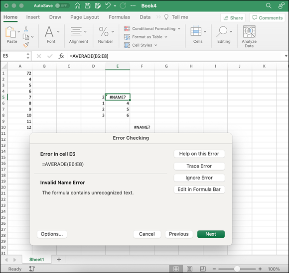
FIGURE 14-13: Use the Error Checking dialog to easily locate problematic formulas.
Use the following buttons in the Error Checking dialog to locate the error’s cause and fix the formula:
- Help on This Error: Invokes Excel’s Help system, taking you to the page discussing the particular error type
- Trace Error: Draws a box around the cells in the argument list and an arrow pointing to the formula
-
Ignore Error: Does just what you’d expect from its name
 Ignoring some errors, such as when a formula doesn’t include adjacent cells containing data, removes the error indicator; however, if a real problem exists, such as a syntax error, the error indicator remains.
 - Edit in Formula Bar: Dismisses the Error Checking dialog and places your cursor in the formula bar so that you can make corrections
- Options: Presents the Error Checking pane in the Excel Preferences dialog
- Cancel: Dismisses the Error Checking dialog
- Previous/Next: Moves to the previous or next error, if one exists
 Error Checking works on only the active sheet in your workbook. If you want to check other sheets, select them and reinvoke the Error Checking dialog by choosing Tools ⇒ Error Checking.
Sorting and Filtering Data
One common use for Excel is as a list manager (a simple database). Every column is a field, and every row is a record. (Okay, every row other than the first is a record if the first is used to display field names. Excel calls it a header row.) Examples of such lists are inventories of personal possessions (for example, vinyl records, which are once again in vogue), membership lists, or bridal registries. In fact, many of the online templates discussed earlier in this chapter are simple databases (lists). Excel’s powerful searching and sorting features that we're about to help you explore, along with Excel’s formulas to calculate values based on the data you enter, make Excel an excellent vehicle for this type of list management.
Sorting data
When presenting list data, you often need to display it in a sorted order. For example, when listing contact information, occasionally you want to sort by surname, zip code, or company or department. Excel makes these types of sorts easy to accomplish. Just follow these two steps:
-
Select a cell in the column you want to sort.
If you select the column header rather than a cell, Excel gives you the option to sort only the contents in the selected column or to expand your selection so that data in other columns is sorted to track with the first column.
-
Click the down arrow next to the Sort & Filter button on the ribbon’s Data tab and choose Sort Smallest to Largest or Sort Largest to Smallest from the pop-up menu.
Your records (the rows) are now rearranged with the sort column controlling the order in which they appear.
 If your sort column contains numbers, the sort order depends on whether the cells are formatted as text or numbers. If the data is simply text composed of digits (that is, it’s left justified in the cells), you might not get the result you expect. For example, 11 precedes 2 when sorted textually. When you want to sort numbers, make sure that the cells in the column are formatted as numeric data.
Using filters to narrow your data searches
Another common database or list operation is to search for only those records that meet specific criteria. (For example, a library might use this type of operation to create a list of all its hardback books.) These searches filter out records that don’t match your criteria, which is why Excel calls these searches filters.
To perform a simple filtering operation, follow these steps:
- Click in any cell in your list.
-
Click the Sort & Filter button on the ribbon’s Home tab and click the Filter button. Or click the Filter button on the Data tab (shown in Figure 14-14).
Filter arrows appear at the top of each column.
-
In the column heading for the data you want to filter, click the filter arrow.
A dialog appears, as shown in Figure 14-14.
- Click the Choose One pop-up menu and then click a criteria to select it.
-
Click the value pop-up menu and select a value from the list.
Rows that don’t match your filter criterion are hidden until you choose to show them again (by clicking the filter arrow again and choosing Clear Filter).
The Filter arrow turns into a tiny filter icon for a column that has a filter applied. Also, the row numbers for those rows matching the filter are displayed in blue.
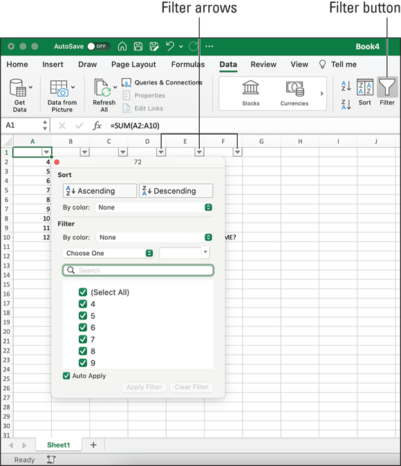
FIGURE 14-14: Filter arrows appear at the top of a list column.
Finding and Replacing Data
As your worksheets fill with data, locating a particular number or piece of text can become problematic. Although Excel filters are useful for finding values in the columns of a list, not all worksheets are lists. If you want to find a particular number or text string wherever it occurs in your worksheet, a more generic searching capability is required. As usual, Excel provides commands to facilitate your searches.
You can search a cell range, sheet, or workbook for a target number or text. To do so, follow these steps:
- If you want to search a cell range, select the range; otherwise, click in any individual cell to search either the sheet or the entire workbook.
-
Choose Edit ⇒ Find ⇒ Find.
The Find dialog (seeing a pattern yet?), shown in Figure 14-15, appears.
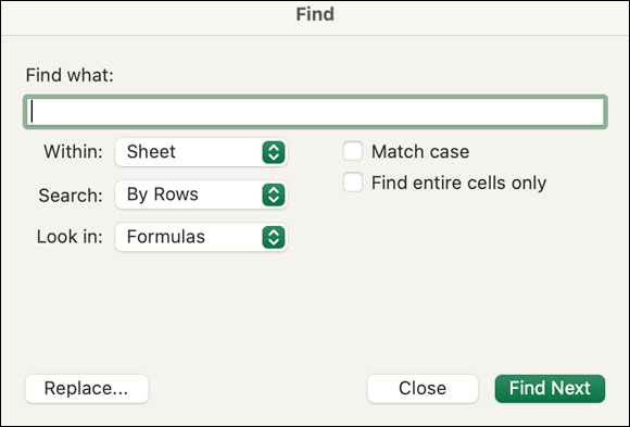
FIGURE 14-15: Search for specific values in the Find dialog.
-
In the Find What text box, enter the target text or number.
Excel supports these three wildcard characters in your search string: - Question mark (?): Matches any single character. For example, entering a?m matches alm, arm, asm, and abm.
- Asterisk (*): Matches any number of characters (0 or more). For example, entering a*m matches am, alm, and accum.
- Tilde (~): Precedes a question mark or asterisk to find that character. For example, enter abc~? to match abc?.
- (Optional) Choose from the following pop-up menus or check boxes to refine your search:
- Within: Specify whether to search only in the current sheet or all sheets in the workbook.
- Search: Search by row or column.
- Look In: Restrict your search to formulas, values, notes, or comments.
- Match Case: Select this check box to make a text search case-sensitive.
- Find Entire Cells Only: Select this check box to confine the search to exact matches — for example, a search for Frank doesn’t match a cell containing Frank Sinatra.
- Click Find Next.
- When you’re finished, click Close.
Closely related to searching text is replacing it. To find one piece of data and replace it with another, proceed as follows:
- To search a cell range, select the range; otherwise, click any individual cell to search either the sheet or the entire workbook.
-
Choose Edit ⇒ Find ⇒ Replace.
The Replace dialog appears, as shown in Figure 14-16.
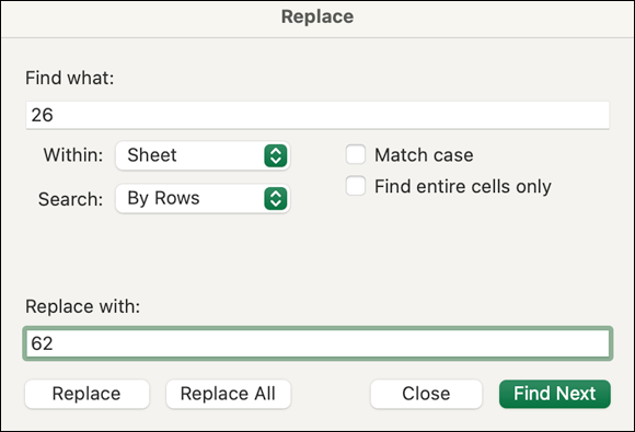
FIGURE 14-16: Similar to the Find dialog, the Replace dialog lets you find data and specify replacement values for that data.
- In the Find What text box, enter the target text or number.
- in the Replace With text box, enter the replacement value.
-
(Optional) Choose from the Within pop-up menu to specify whether to search only in the current sheet or all sheets in the workbook.
Choose from the Search pop-up menu to search by row or column. The Match Case check box makes a text search case-sensitive, and the Find Entire Cells Only check box confines the search to exact matches. (For example, a search for Elvis doesn’t match a cell containing Elvis Presley.)
- Click Find Next.
- If you want to replace the found value with your replacement value, click Replace.
- Repeat Steps 6 and 7 as often as you want.
- (Optional) To perform a blanket replacement without inspecting the found values, click Replace All rather than perform Steps 6 through 8.
- When you're done, click Close.