
Chapter 16
Advanced Spreadsheeting
IN THIS CHAPTER
![]() Making Excel your own
Making Excel your own
![]() Using conditional formatting
Using conditional formatting
![]() Giving cell ranges memorable names
Giving cell ranges memorable names
![]() Adding multiple sheets to a workbook
Adding multiple sheets to a workbook
![]() Including hyperlinks
Including hyperlinks
![]() Collaborating with others and turning on revision tracking
Collaborating with others and turning on revision tracking
Excel is the industry standard spreadsheet application — the one to which every other spreadsheet is compared — for a reason. Thus far, all challengers have come up short. Microsoft introduced Excel (on the Mac, first) back in 1985, replacing its Multiplan spreadsheet. One of Excel’s biggest features in the early days was that it was the first to let the user alter a sheet’s appearance by supporting multiple fonts, character attributes, and shading. Microsoft continued adding features, allowing users to control more of Excel’s functionality, including extensive automation capabilities.
In this chapter, you find out how to customize Excel to make it work like you want it to, use multiple sheets in a workbook, and add hyperlinks to spreadsheets. You also learn how to collaborate with others to combine your spreadsheet talents.
Customizing Excel
Microsoft has gone to great lengths to make Excel look, feel, and behave like a natural part of your macOS experience. Tailoring Excel’s appearance and behavior to fit your work style and sense of aesthetics falls into two major areas: preferences and the Excel toolbar and menu system.
Preferences
The Excel Preferences dialog (choose Excel ⇒ Preferences or press ⌘ +comma), shown in Figure 16-1, bears a strong resemblance to the macOS System Preferences window. You can find most customization options in this dialog’s various panes (which appear when you click the corresponding icon in this dialog).
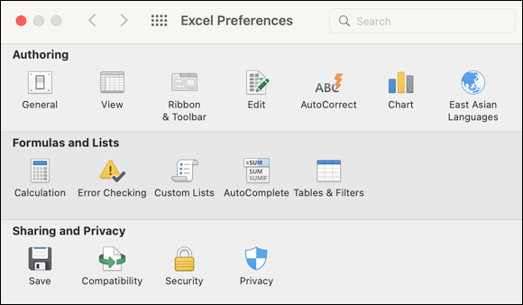
FIGURE 16-1: Is it System Preferences, or is it Excel Preferences?
Excel lets you tune its appearance and behavior to suit your style and usage. You get a plethora of choices in the various categories.
Covering every option in detail would add so many pages to this book that you’d need a crane to lift it. We hit only a few of the preferences you might want to find quickly. Besides, every preference pane has a Description box, which displays useful information about any option over which you hover the cursor.
General pane
The General pane, which you can access by clicking the leftmost button on the Authoring row (labeled General), includes a few especially useful preferences:
- Use R1C1 Reference Style: Unless you’re incredibly comfortable with alternative numbering systems, you probably think C1024 is a more comprehensible name for the 1024th column than AMJ. Selecting the R1C1 check box bypasses the mental gymnastics of performing base 26 arithmetic (with letters substituting for numbers) to specify a column name and lets you use standard decimal numbering preceded by R (for row) and C (for column) when designating a cell (or row or column).
- Default Font: As its name implies, use this text box (or the associated pop-up menu) to specify your preferred font. The default is the aptly named Body Font — better known as Calibri. (You can also specify a default size for your chosen font by using the Font size text box and pop-up menu.)
- Show Workbook Gallery when Opening Excel: If you work primarily with existing documents and find the Workbook gallery an unnecessary addition when you first launch Excel, deselect this check box and the application immediately displays a new, blank workbook.
- Confirm before Opening Other Applications: We like to enable this option so that if we don’t intend to open another application (such as opening a web browser by accidentally clicking a hyperlink in a spreadsheet), we can simply deny the action and stay in Excel.
View pane
The View pane controls what Excel features are visible and how some features are displayed. You find options in these boxes to establish default behaviors:
- Show in Workbook: You can hide or show the formula bar, sheet tabs, headers, and other items, as well as specify whether new sheets appear in normal or page layout view. Excel’s default is to display new sheets in normal view.
- For Cells with Comments, Show: Controls whether and how comments are shown. See the section “Collaboration and Revision Tracking (a.k.a. Change Tracking),” later in this chapter, for a discussion of comments.
- For Objects, Show: Controls whether non-cell data, such as graphics, charts, text boxes, and others, are shown in their entirety, displayed as gray rectangles (indicators), or hidden.
- In Ribbon, Show: Hide or show the Developer tab and Group Titles. Selecting the Developer tab check box displays the Developer tab on the ribbon, from which Excel pros can utilize Visual Basic and other advanced tools.
Ribbon & Toolbar pane
You’re unlikely to find a model home in which every aspect is exactly the way you want it. The home might be slightly more expensive than is comfortable, you might want to repaint a room, or you might decide to replace the living room carpeting. A perfect match is rare. Like the model home, Excel might be close to what you want but still leave you feeling the need to tweak it. For example, you might find Excel’s ribbon and its menus cluttered with features you don’t need (if, say, you use Excel almost exclusively as a list manager, you probably don’t need pivot tables). Similarly, you might want a single location that contains the tools and commands you use most often. Look no further than the Ribbon & Toolbar pane for such customizations.
As discussed in Chapter 3, you can customize the dickens out of the ribbon and toolbar in Microsoft Office apps, and Excel is no exception. This preferences pane affords two tabs: one for customizing the ribbon itself and its commands, and another for customizing the Quick Access toolbar, which resides at the top of every Excel workbook window.
Edit pane
The Edit pane controls how Excel behaves while you’re editing a sheet (for example, when you enter data and how you interact with cells). One option on this pane allows you to specify how Excel interprets two-digit year values when you enter a date. By default, Excel interprets 00 to 29 as 2000 to 2029 and 30 to 99 as 1930 to 1999.
AutoCorrect pane
In the AutoCorrect pane, you can access the Excel subset of Word’s AutoCorrect preferences. Check out Chapter 6 for the scoop on Word’s AutoCorrect.
Chart pane
The Chart pane has only two options, and both pertain to showing information in charts when you roll your cursor over the various elements within them. One option allows you to see the names of elements, and the other displays data point values.
East Asian Languages pane
Microsoft Office supports the use of East Asian languages, but the feature must be enabled from this pane. Choose Japanese, Simplified Chinese, or Traditional Chinese from the Select a Language pop-up menu, and then restart Excel to apply language-specific features.
Calculation pane
The Calculation pane, which appears when you click the Calculation button in the Formulas and Lists row, has two sections:
- Calculation Options: Specify whether formulas recalculate automatically (for example, when any referenced cell’s value, name, or formula changes). The default is Automatic, but you can choose Automatic Except for Data Tables or Manual. Use the Iteration controls to limit how many calculations Excel performs when it encounters a circular reference or performs a goal-seeking calculation. (The default is 100.) Similarly, you can tell Excel to stop recalculating when results differ from the previous result by less than a set limit. (The default is 0.001.)
-
When Calculating Workbooks: Specify whether to use the 1904 date system (the date system based on the Macintosh system clock, in which time began at midnight, January 1, 1904). You can also have Excel store values retrieved from external links (the default setting). By default, Excel stores everything to 15 decimal places; however, if you select Set Precision as Displayed, Excel stores only as many decimal places as you set for display precision. (The default display precision can be set in the Editing preferences pane.)
 If you’re not absolutely sure you need it, we suggest that you don't use the Set Precision as Displayed option. You could end up losing data you later find you needed.
Error Checking pane
The Error Checking pane controls which errors are flagged. (See Chapter 14 for more details about error checking.)
Custom Lists pane
In the Custom Lists pane, you can add to the four custom lists with which Excel ships. See Chapter 15 for a fuller discussion.
AutoComplete pane
AutoComplete preferences tell Excel when and how to suggest values while you type, such as for function names (see Chapter 14) and text values.
Tables & Filters pane
By default, Excel references table names in formulas and resizes tables automatically if they span more than one column or row. You can turn off this perfectly legitimate behavior from the Tables section of this preferences pane. The Filters section of this pane has just one setting: By default, Excel displays dates grouped by year/month/day in a filtered column. Disable the Group Dates when Filtering check box to turn off this feature.
Save pane
The third preferences category, Sharing and Privacy, includes the Save preferences pane, in which you can tell Excel whether you want Autosave enabled by default (we’d heartily recommend that you leave this option selected) and whether you want it to save a preview picture for new files.
Compatibility pane
The Compatibility pane is a major destination, especially if you plan to share your workbooks with other users. In addition to pointing out when you use features not available in other Excel versions on either the Mac or Windows, the pane enables you to specify the default file format in which Excel saves workbooks. By default, Excel saves workbooks in .xlsx format (an XML-based format introduced in Excel 2007 on Windows), but if you need to interact with users of much older versions (which is fairly rare these days), you should probably opt for the older .xls format, used by Excel 97 through Excel 2004. (Other formats are available, including various interchange formats, such as comma-delimited text.)
Security pane
In the Security pane, you can set Excel to remove personal information (such as the authorship information on the File Info Summary tab), and activate a warning that appears when you’re opening a workbook that contains macros. If you use the Enable All Macros option, you can be a Typhoid Mary, passing on macro viruses to others who may use macro-enabled files.
Privacy pane
The Privacy pane allows you to opt in or out of cloud-based connected experiences across the devices with which you use Microsoft Office products.
Conditional Formatting
Excel, like other spreadsheets, has its genesis in VisiCalc, an electronic ledger. One common practice in ledgers is to use different ink colors to highlight specific characteristics. For example, red ink can indicate a loss or negative value, and black ink can indicate a positive value. These color uses have become part of common English vernacular — something’s “in the red” when it’s losing money and “in the black” when it’s showing a profit.
Excel takes the “in the black/in the red” metaphor a little further with conditional formatting, with which you can specify formatting attributes that you want to apply to a cell’s contents based on the cell’s value or on a formula you define.
To apply conditional formatting to a cell, proceed as follows:
- Select the cell(s) to which you want to apply conditional formatting.
-
Choose Format ⇒ Conditional Formatting.
The Manage Rules dialog appears (see Figure 16-2).
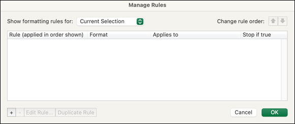
FIGURE 16-2: Use the Manage Rules dialog to add conditional formatting rules.
- To add a new formatting rule, click the + (add) button.
-
To change the default two-color scale, click the Style pop-up menu to specify icons, data bars, the three-color scale, or Classic style (a single color).
The settings you see change according to the style you’re using.
-
If necessary, to specify the target values for the cell, use the options in the Minimum and Maximum sections.
Again, Excel displays different settings depending on the choice you made on the Type pop-up menu in the Minimum and Maximum sections. Figure 16-3 illustrates the default rule, which is based on lowest and highest values in a cell — therefore, you don’t have to enter a minimum or maximum value for the default rule.
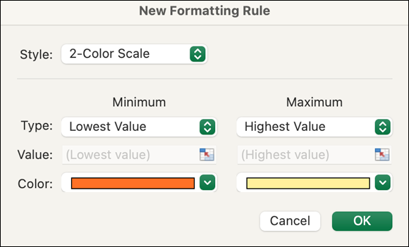
FIGURE 16-3: In the New Formatting Rule dialog, you can configure conditional formatting.
- Click each of the Color pop-up menus and select colors.
- Click OK.
- (Optional) To set additional conditions, click the + (add) button.
- When you’re done, click OK to dismiss the Manage Rules dialog.
 You can apply multiple conditional-formatting rules to the same range or to overlapping ranges. More than one of your conditions can evaluate to true; however, Excel applies only the formatting for the first true condition, so the order in which you define your criteria matters.
 You can also create conditional formatting rules by clicking the Conditional Formatting icon on the ribbon’s Home tab and using the pop-up menus that appear.
You can copy conditional formatting by using the Format tool, as with any other cell formatting. (See Chapter 14 for details on how to use the Format tool to copy a cell’s formatting.) So, after you have a set of criteria you like, you can apply them to additional cells by selecting the cells with the conditional formatting, clicking the Format tool, and dragging across new cells to which you want to apply the formatting.
To modify or remove a conditional formatting criterion, choose Format ⇒ Conditional Formatting and make your changes in the Manage Rules dialog that appears. (You can change the applied formatting by clicking Edit Rule.) To delete a conditional formatting rule, click it in the list to select it, and then click the − (delete) button.
To completely remove conditional formatting from cells, select the cells and choose Edit ⇒ Clear ⇒ Formats.
Naming a Cell Range
A cell's name is called a cell reference. Cell reference nomenclature can be either R1C1 (for example, R31C27) or column letter/row number (for example, AA31 for column 27, row 31) format, depending on your General preferences setting. However, when you’re working with your data, you probably think of a group of cells that contain inventory unit costs as something like Unit_Costs, not as B5 through H5. You might even place a text label in A5 that says Cost_per_Unit so that when other people look at your sheet, they know what the numbers mean.
You can assign a name to a cell or a range of cells and use that name in formulas rather than use the less descriptive cell references. To name a cell range, follow these steps:
- Select the cells you want to name.
-
In the formula bar’s Name box (the box at the far left end of the bar), type a descriptive name for your selection.
Names must start with a letter or an underscore; consist of only letters, digits, periods, or underscores; be different from any cell reference; and be no longer than 255 characters. You can use both uppercase and lowercase characters, but Excel treats names as case-insensitive, so unit_cost and Unit_Cost are considered the same name.
You can now reference the cell range by name in formulas. For example, entering =AVERAGE(Unit_Cost) in the preceding example is the same as entering =AVERAGE(B5:H5), but you can more easily recognize which cells the first formula is describing.
Working with Multiple Worksheets
Excel workbooks can contain more than one sheet. In fact, previous versions of Excel defaulted to three sheets in newly created workbooks. (Excel defaults to one, but you can change that number in Excel’s General preferences pane by typing a new value into the Sheets in New Workbooks text box.) Also, you can add sheets to your existing workbooks when you have the need (or desire). You may wonder why you’d want multiple sheets in a workbook. There are as many answers to that as there are to why you’d want to have multiple pages in a notebook. A teacher might want a grade book that contains one sheet for every class taught — keeping related data in one file is surely more convenient than managing multiple files. Or you might want to consolidate your financial data into one book, with separate sheets for checking accounts, savings accounts, brokerage accounts, and credit cards.
Excel offers many ways to add sheets to an existing workbook:
- Choose Insert ⇒ Sheet and then choose the type of sheet from the submenu that appears: Insert Sheet (Blank) or Chart Sheet.
- Click the + (plus) tab near the bottom of the workbook window to add a new, empty sheet.
- To add a new, empty sheet, right-click any sheet’s name tab and choose Insert from the shortcut menu that appears.
You don’t have to live with only the generic Sheet-n name that Excel provides. You can double-click the text on the sheet’s name tab to highlight it and type a new name. Or you can choose Rename from the shortcut menu that appears when you right-click the sheet’s name tab. Again, the name becomes highlighted, and you can type a new name.
Excel cell reference notation can handle references to cells on other sheets and even in other workbooks. For example, you can reference cell C2 on Sheet2 in a formula on Sheet1 by using the notation Sheet2!C2. In other words, precede the cell reference with the sheet name (enclosing it in quotes if it contains spaces) and an exclamation point. To reference cells in another workbook, you can enclose the workbook name in square brackets, followed by the sheet name, an exclamation point, and then the cell reference. For example, “[GradeBook]SecondPeriod!C2” references cell C2 on the sheet named SecondPeriod in the workbook named GradeBook.
For workbooks that aren’t open, the full file system path to the workbook precedes the filename. Thus, the following line:
'BobsLion/Users/BobLevitus/Documents/Workbooks/[DVDs]Backups!Latest'
might refer to a cell in which you record the disk name, date, and time of your last data backup (yes, backing up your data is important!) in a workbook that contains your DVD inventory.
Hyperlinking
As with the other apps in Microsoft Office, you can insert hyperlinks in Excel. These links can redirect you to a web page; create a preaddressed email message; or open another Office document, prepositioned to the referenced text (in Word), cell (in Excel), or slide (in PowerPoint).
Creating a hyperlink to an Excel cell or object is easy. Just follow these steps:
- Select the cell or object that you want to become the hyperlink.
-
Choose Insert ⇒ Hyperlink (or press ⌘ +K).
The Insert Hyperlink dialog appears (see Figure 16-4).
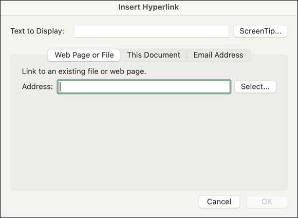
FIGURE 16-4: Define your hyperlinks in the Insert Hyperlink dialog.
-
Select the tab for the type of link you want to create.
For the purpose of this example, we're linking to a specific cell in the Excel workbook we're working in, so we select the This Document tab. The options in the Web Page or File and Email Address tabs work similarly.
- Type the cell reference (or select from the named documents and defined names in the dialog’s lower list), as shown in Figure 16-5.
-
(Optional) In the Display text box, make the display text more descriptive, such as Total Assets or Stock on Hand, if you want.
You can also attach a ScreenTip that appears whenever the cursor hovers over the link. Click the ScreenTip button in the upper right of the Insert Hyperlink window. In the dialog that appears, type the text you want displayed in the ScreenTip. - Click OK to dismiss the Insert Hyperlink dialog.
Removing a hyperlink is simplicity itself. Right-click a cell that contains a hyperlink and select Remove Hyperlink from the shortcut menu that appears. Similarly, if you want to modify or otherwise edit an existing hyperlink, right-click the cell containing the hyperlink and choose Edit Hyperlink.
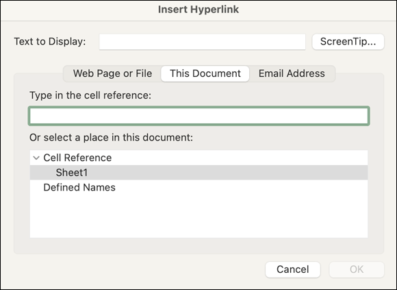
FIGURE 16-5: Type the cell range or select a named range in this dialog.
Collaboration and Revision Tracking (a.k.a. Change Tracking)
Sometimes, it takes a village (or, at least, a group) to create a spreadsheet. If your project requires input from multiple parties, you’ll truly appreciate Excel’s support for collaboration and revision tracking.
When you share a workbook, Excel automatically disables a number of Excel features, including
- Creating or modifying conditional formatting
- Merging cells
- Adding or changing charts, pictures, shapes, and hyperlinks
So, if you want to perform any of these tasks, do so before you turn on change tracking and workbook sharing (or simply don’t even turn them on).
Saving a workbook online
You can save your Excel workbooks to any storage device on your home or office network, as long as you have the proper permissions — but saving that same workbook to OneDrive and sharing it with others allows them to collaborate with you.
To save your workbook to your OneDrive, follow these steps:
- Click the Share button in the upper-right of your workbook’s window to open the Share dialog, shown in Figure 16-6.
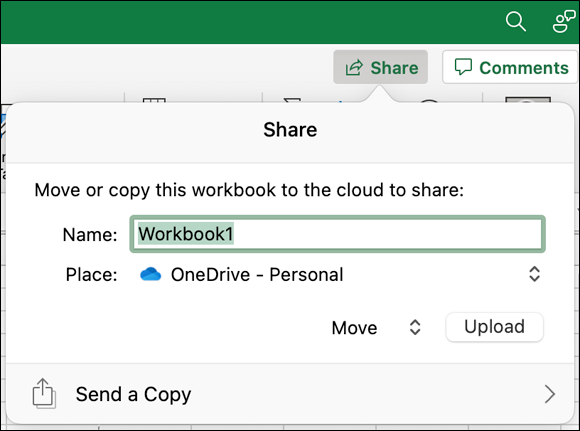
FIGURE 16-6: Saving a workbook to OneDrive is the first step to sharing it.
- (Optional) Type a new filename for your workbook.
- Click a destination OneDrive account for the file (if you have more than one, perhaps for personal use or business).
-
Choose Move or Copy from the pop-up menu to the immediate left of the Upload button.
Move will move the file from its present location to your OneDrive account, while Copy will make a copy of it instead.
- Click Upload to upload the file to your OneDrive.
To share your uploaded workbook with others:
-
Click the Share button in the upper-right of your workbook’s window to open the Share dialog, shown in Figure 16-7.
Note that the Share dialog offers different options than it did in Figure 16-6. That’s because the file has already been uploaded to OneDrive.
- Choose a method for sharing your file with others:
- Invite People: Click Invite People, enter the names of people in your Apple Contacts app or just type their email addresses, add a message if you like, and then click the Share button. If you want them to be able to edit your workbook, be sure to check the Can Edit box before clicking Share.
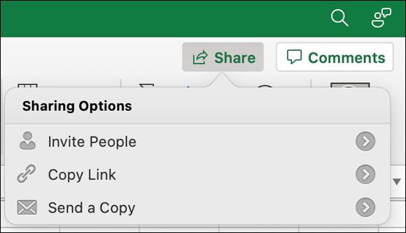
FIGURE 16-7: Share your uploaded workbook via OneDrive.
- Copy Link: Copy a link for the shared file to your Mac’s clipboard, which you can then paste the link into documents, emails, websites, and so on. Click Copy Link, and then select View-Only (to allow only those you share with to view the workbook) or View and Edit (to allow others to edit your workbook).
- Send a Copy: Send a copy of the workbook file as an Excel workbook or as a PDF to others via email.
- Invite People: Click Invite People, enter the names of people in your Apple Contacts app or just type their email addresses, add a message if you like, and then click the Share button. If you want them to be able to edit your workbook, be sure to check the Can Edit box before clicking Share.
Tracking your changes
To track changes, choose Tools ⇒ Track Changes ⇒ Highlight Changes. In the Highlight Changes dialog that appears (see Figure 16-8), make sure that the Track Changes While Editing check box is selected. (Otherwise, Excel doesn’t save changes for you to view, accept, or reject later.)
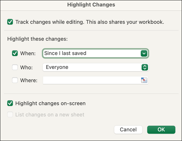
FIGURE 16-8: The Highlight Changes dialog lets you highlight changes during a specific period, by a specific user or users, or to a specific cell range.
When the Highlight Changes on Screen check box is selected (which it is by default), the changes appear in a ScreenTip whenever you hover the cursor over a change. A changed cell has a dark blue triangle in its upper-left corner, similar to the triangle indicating a formula error. (See Chapter 14 for more about Excel’s error checking and marking.) Selecting the List Changes on a New Sheet check box tells Excel to create a history sheet for the change log (a textual history of all changes made).
You can’t log changes to a new sheet until the workbook has been saved with the Track Changes While Editing check box selected. After you turn on change tracking, save the workbook by clicking OK in the Save dialog that appears and then choosing Tools ⇒ Track Changes ⇒ Highlight Changes again. In the dialog that appears, select the List Changes on a New Sheet option. Yeah, this procedure is cumbersome, but not everything in life (or Excel) is easy.
Accepting and rejecting your changes
Now comes the payoff. You can review your changes and accept or reject them, either individually or all at the same time. Here’s how:
-
Choose Tools ⇒ Track Changes ⇒ Accept or Reject Changes.
Excel might prompt you to save your workbook at this point. If it does, go ahead and save your workbook.
The Select Changes to Accept or Reject dialog appears, as shown in Figure 16-9.
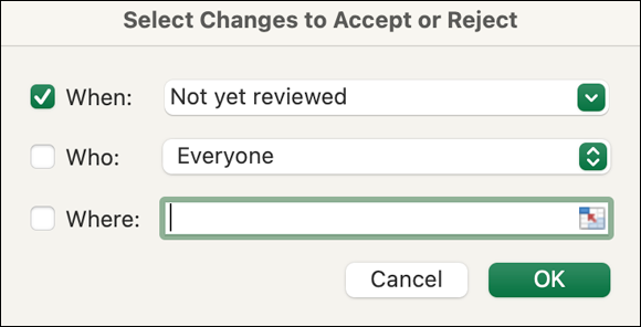
FIGURE 16-9: Specify the group of changes you want to check for.
-
Specify the types of changes you want to consider.
The default is All, but you can limit the considered changes to a specific user, time frame, or cell range by choosing from the pop-up menu and clicking OK.
The Accept or Reject Changes dialog appears (see Figure 16-10).
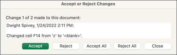
FIGURE 16-10: Step through the change history in the Accept or Reject Changes dialog.
-
Click the Accept or Reject button for each change.
Excel proceeds to the next change. Alternatively, you can click Accept All or Reject All to have Excel perform a blanket acceptance or rejection of all subsequent changes, without your input for each individual change.
-
Click Close when you finish.
The Accept or Reject Changes dialog closes, and you return to your worksheet.
With this sort of control, you can relate to the Mel Brooks line in History of the World, Part I — “It’s good to be the king!”