CHAPTER

5

Planning and Sizing
the Enterprise VM
Server Farm

One of the most important steps in configuring the Oracle Enterprise VM farm is planning, which involves all aspects of both sizing and configuration. Sizing is the art and science of determining the amount of hardware required for a system you are configuring. A mistake or underestimation of needed resources could cause significant problems later on when performance is an issue. In this chapter, you will learn how to plan and size the Oracle Enterprise VM farm.

Planning the VM Server Farm

You have several choices to make when planning the VM farm, including the number of servers, their configuration (server pool masters or virtual machine servers), and their sizing. Before getting started, let’s look at the definition of a Oracle VM server farm.

Server farm is another term for data center. The server farm is a collection of systems used to serve an enterprise when the use of one system will not provide sufficient capacity needed to support the enterprise. Thus, the Oracle Enterprise VM farm is the collection of systems used to support the virtualization needs of the Oracle Enterprise. The Enterprise Oracle VM farm can be made up of one or more Oracle VM server pools, which are made up of one or more Oracle VM servers.

One Pool or Multiple Pools

From a high level, it might appear that putting all of the Oracle VM servers into the same server pool would be most efficient. This is certainly an efficient way to manage all of your resources with the least effort because all the VMs can now run on all the underlying hosts. However, a few other concerns might make this impossible.

When planning the server pool, keep in mind that there are nonclustered server pools and clustered server pools. Let’s look at these different types of server pools.

Nonclustered Server Pool

The nonclustered server pool is made up of a collection of VM servers that use NFS for shared VM storage. The nonclustered server pool can be made up of one or multiple VM servers. If you chose to use shared filesystem storage, the server pool must be clustered. The nonclustered server pool does not support High Availability (HA).

Clustered Server Pool

The clustered server pool uses shared cluster storage and the cluster quorum to maintain the cluster. In the event of a server failure, the virtual machines from the failed server will automatically restart on existing servers in the cluster. As with the nonclustered pool, the clustered pool can be made up of one or multiple servers.

All the nodes of the cluster must reside on the same shared storage, thus maintaining the cluster. An interesting option is to locate some of the servers in another part of the data center or another building in order to create a stretched pool. As long as storage is accessible from the stretched nodes in the server pool, this will maintain a higher level of HA.

Although the stretched pool is not completely supported, it does work and can be implemented. Keep in mind that there might be some performance degradation for the remote nodes.

Server Pool Configuration

First, all the systems in the VM server pool should be running on the same hardware. The Oracle VM Manager will not prohibit mixed server pools, but they really aren’t a good idea because of the problems you might run into. Some features, such as the HA Auto-Restart feature, will work even if the servers are not the same architecture because the HA enabled feature will start the system from a cold state; however, live migration will not work. Also, all the systems in the server pool must have the same basic hardware architectures.

Second, all the systems in the VM server pool should support the same level of hardware virtualization. Many systems remain in production that are 64 bit but do not support hardware virtualization. It is not recommended that the two processor types be configured in the same pool. If only paravirtualized guests are being used, mixing both systems with hardware virtualization support and hardware without hardware virtualization support is feasible. In addition, features such as HA enabled, live migration, and HVM will dictate whether a mixed environment can be used.

Sometimes it’s not easy determining what type of processor you have and what support is available for virtualization. In the case of the Intel chipset, an easy-to-use web page that can help you is available: http://ark.intel.com. From here, you can determine the support available for your system. For example, I retrieved the following information from /proc/cpuinfo:

Intel(R) Xeon(R) CPU            X5670  @ 2.93GHz

I then entered the model number X5670 on the Intel website and, among other information, obtained the following:

Intel® Virtualization Technology (VT-x) ‡
Intel® Virtualization Technology for Directed I/O (VT-d) ‡
Intel® VT-x with Extended Page Tables (EPT) ‡

This information tells you that the processor on this system is capable of supporting hardware-assisted virtualization. You can find similar information on the AMD website at http://www.amd.com/en-us/solutions/servers/virtualization.

Once you’ve resolved hardware compatibility issues, you need to decide whether to create one large server pool or several server pools.

Single Server Pool

The primary reason for creating a single server pool is simplicity, which means easier configuration and administration. Because everything is in a single server pool, you have a single set of templates and images as well as a single storage system. Moving any virtual machine to another system in the server pool is easy, and failover is straightforward. A single server pool means less work to manage, seeing as you have one master and one or more VM servers all grouped together. The only real planning challenge is in the sizing of the server(s).

The downside of having a single server pool is that several maintenance tasks require the entire server pool to be rebuilt. These maintenance tasks can cause some loss of service to the server pool while the maintenance is being done. If you have multiple server pools, you can maintain one server pool at a time. These tasks include the following:

   Changing the OCFS2 cluster timeout

   Moving the OCFS2 cluster heartbeat to a different Oracle VM network

   Changing the NFS filesystem used for a pool file system

   Changing the SAN device used for the pool file system

   Changing the hostname/IP of an NSF file server used for a pool file system

   Recovering from a corrupt pool file system if no backup exists

   Converting a nonclustered sever pool to a cluster server pool

In the next section, you will learn the advantages of multiple server pools.

Multiple Server Pools

Using multiple server pools makes sense for a lot of installations for several reasons. Some of the reasons are technical, but others are purely a matter of politics and/or policy considerations. Having multiple server pools means having multiple sets of storage and multiple sets of servers; however, you can still manage them with the same VM Manager. You can also create multiple VM Managers if desired.

One of the primary reasons for separate server pools is separation of data. Many enterprise security policies require data from different departments or sometimes even require different projects to be stored separately. This is especially true in the government, where data secrecy might demand separation of data. This separation of data is accomplished by configuring separate server pools.

Another reason for having separate server pools is Quality of Service (QoS). Dividing components into separate server pools based on different levels of performance, uptime, monitoring, and management is quite common. The higher the QoS, the more you would typically pay for that service. It makes sense to pay only for the service level you require. For example, getting less service for testing, development, and training environments than for the production environment is okay.

To create separate service levels, split the virtual machines into different server pools. The various server pools might have different numbers and types of servers, different storage, and more networking equipment based on the level of service required. A server that guarantees a higher level of service might allocate fewer virtual machines per CPU than one with a lower guaranteed performance level. This is true of storage as well.

Another reason for separate server pools is to separate environments based on access and function. Thus, production, testing, and development can be allocated in separate server pools, which helps guarantee there is no unintended access or overlap. This allows you to create a barrier between environments. This architecture provides security as well as isolates performance issues into their own environments.

Regardless of your reasons, if you decide to create multiple server pools or a single server pool, you must plan. Planning must include sizing and determining the number of systems for the server pool master, utility servers, and virtual machine servers.

Planning the Server Pool

You have multiple ways to set up the server pool. The server pool is composed of one server pool master and one or more virtual machine servers. Even though the systems are configured as different server types, the software installed is identical; in fact, the server is not designated a server type until you’ve configured it. Therefore, each server starts out identically and is configured as a specific server type. The three server types are server pool master, utility server, and virtual machine server. A VM Server can be designated to perform a single server role, two roles, or all three roles.

Server Pool Master

One server is designated as the server pool master. As you’ll recall, the server pool master is simply a specific component of the VM Agent. The server pool master is the communication conduit between the VM Manager and the Agent, as well as the interface to other Agents on other VM servers. The server pool master is automatically assigned and managed, with no manual intervention required. The server pool master manages load balancing, among other functions. When the administrator requests that a virtual machine start, the server pool master determines which virtual machine server is the least loaded and dispatches the request to start the virtual machine. Typically, the server pool master is also a utility server or a virtual machine server as well, unless it is a server pool master for a large and very busy pool.

With Oracle VM 3.4, the server pool master server role has been deprecated. In OVM version 3.4 and later, the agent communicates directly with the VM Agent on each of the OVM servers. However, because this book covers OVM 3.x, we will continue to refer to the server pool master role.

Virtual Machine Servers

The virtual machine server is really what Oracle VM is all about. This is the server that supports the hypervisor and runs virtual machines. All servers are VM servers by default. There are one or more virtual machine servers in a server pool. The number and type of virtual machine servers is determined by the number and type of virtual machines that need to be supported. When an administrator requests that a virtual machine start, the server pool master determines which virtual machine server has the most resources available and starts the virtual machine there. If a virtual machine server is not found with sufficient resources, an error is returned to the VM Manager.

Utility Servers

The utility server is a server that is chosen to perform more specific tasks in the VM server farm. This server performs tasks such as pool filesystem operations and updating the cluster configuration as well as importing virtual machine templates and virtual appliances and creating virtual machine templates from virtual appliances. It is also responsible for creating repositories. By default, all servers are utility servers. If a utility server is not available, a VM server will be used.

Server Pool Configurations

You can set up server pools in the following ways: All-in-One configuration, Two-in-One configuration, and the individual configuration. Which configuration you decide to use depends on the size of your configuration.

All-in-One Configuration

The All-in-One configuration is the most straightforward configuration. It is made up of the server pool master and virtual machine servers, all residing on the same VM server. This configuration functions well for either a VM farm where there is only a single or a few servers or a configuration where many virtual machines are managed but there are very few changes.

The All-in-One configuration can consist of a single server, as shown in Figure 5-1, or of a single server that supports the server pool master, utility server, virtual machine server, and one or more additional virtual machine servers, also shown in Figure 5-1.

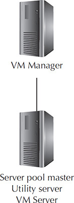
FIGURE 5-1.    All-in-One configuration plus VM Manager

With Oracle VM 3.4, because there really isn’t the concept of the server pool master, all VM servers use the All-in-One configuration.

The advantage of the All-in-One configuration is that configuring and managing it is easy. This configuration does have a disadvantage in that there is a single point of failure if the single Oracle VM Server were to fail (if there is only one). This configuration is becoming more common as hardware is released that is capable of supporting enormous numbers of virtual machines.

Because you can easily add additional virtual machine servers to a server pool (assuming the storage used is capable of being shared), you can always start with an All-in-One configuration and add to it as needed.

Two-in-One Configuration

The Two-in-One configuration involves setting up the server pool master and utility server on the same server. The Two-in-One server configuration is for larger configurations where separating the virtual machine server from the server pool master is necessary. The Two-in-One configuration is shown in Figure 5-2.

FIGURE 5-2.    The Two-in-One configuration

The Two-in-One configuration makes sense where the VM server farm is moderately sized and you need to separate administrative functions from virtual machine functions. If the separation is for preference rather than load, you can configure the server pool master and utility server system as a smaller server than the virtual machine servers.

The type of configuration you choose is partially based on the capacity you need for the VM server farm and partially based on anticipated growth of the farm. Fortunately, if you decide to change things later, this is one area where modifications are easy. This configuration is no longer valid for 3.4 and newer versions of OVM since OVM 3.4 no longer uses the utility server.

Sizing and Capacity Planning

Perhaps more important than the configuration of the VM server farm is sizing and capacity planning for the farm. If the VM server farm is undersized, performance and capacity will suffer and your system will not run at the desired level of service or capacity.

Both sizing and capacity planning are as much an art form as a science. They involve mathematics, monitoring and analyzing of existing workloads, and a lot of extrapolation. Probably more so than most activities, with sizing and capacity planning, the better the data input into the exercise, the better the end result.

In addition to the traditional variables used for sizing and capacity planning, such as the number of servers, number of CPUs, RAM, storage size, and I/O performance requirements, CPU virtualization acceleration features must now be taken into consideration as well. These new virtualization acceleration technologies allow for more virtual machines to be run more efficiently than ever before on the same hardware. In addition, server features such as Non-Uniform Memory Access (NUMA) technology affect performance.

Sizing and capacity planning are among the most challenging tasks you must undertake in planning the VM server farm. As such, they are two of the most important as well. As mentioned earlier, an undersized system will cause performance problems later. In the next sections, both sizing and capacity planning are covered.

Sizing

Sizing is the act of determining the amount and type of hardware needed for a new installation of an application. Sizing differs from capacity planning in that the hardware will be supporting a new application or a new installation of hardware, rather than an upgrade or addition to the existing hardware in a system. For example, if a computer system will be replaced by another system that has more resources or is faster, sizing is involved. If that same system will have more CPUs or more memory added to it, capacity planning is involved. Typically, the components that end up being the biggest bottleneck to the VM server farm are network and storage.

This section assumes that the sizing exercise is geared toward taking nonvirtualized systems and virtualizing them—in other words, taking standalone systems and sizing a virtualized environment to accommodate new virtual machines to run the applications formerly running on the standalone servers. The section on capacity planning is geared toward managing the capacity of an already virtualized environment.

The steps involved in sizing a new system are data collection, analysis, and design. The better the data collection, the better the design will be. Keep in mind that there will still be a lot of work to do in the analysis stage where you analyze and decompose the data.

Data Collection

Sizing the new system starts with collecting as much data as you can about the application and the expected workload. If the new system is a replacement for an existing system, much of this data is readily available. You can collect data by monitoring the existing system. If possible, create specific tests or conditions where a single virtual machine is running, so you can analyze a specific workload.

A few different types of data are collected. Data collection is used to gather information about the workload that will be run. In addition, data is collected about the number and type of virtual machines that will be deployed. Collect this data in a workbook that you can then use to determine the number and size of systems to include in the design.

Workload Data Collection    Collecting data about the required workload is typically done using tools available in the OS that is being deployed with whatever systems are available. If this is a completely new system and there are no available reference systems, sizing is more difficult. As mentioned before, the better the data, the better the result.

If you’re modeling Linux systems, use tools such as sar, top, iostat, and vmstat. These utilities provide information about the system’s current CPU utilization as well as memory utilization and I/O utilization. Collect data over a fairly long period of time, so you can gather both averages and peaks. Collect a minimum of one month of data, though longer is recommended.

If you’re modeling Windows systems, use Performance Monitor (perfmon). Perfmon provides data on CPU, memory, and I/O utilization. You can use this data to help size the new system. Windows perfmon not only is capable of collecting a large variety of data but also is capable of saving it. Its major downside is its inability to export that data in text form.

Requirements Collection    Requirements collection involves interviewing management to determine the number of virtual machines needed and what they will be used for. Certain requirements, such as the number of systems, should be fairly easy to obtain. Other requirements, such as the needed amount of RAM, might be readily available due to specific requirements such as database size, or you might need to ascertain it from the workload data collection.

RAM is one of the most important requirements because Oracle VM does not over-commit memory. Therefore, you must size the host with sufficient RAM to support the sum of the RAM of the individual virtual machines. This differs from some other virtualization products such as VMware, which allow for the over-committing of memory. The designers of Oracle VM and the Xen Hypervisor felt that the over-committing of memory could lead to potential performance problems and that memory is inexpensive enough to make over-committing unnecessary.

In addition to memory, you need to gather CPU requirements. The number of CPUs required for virtual machines might be determined by business rules or workload analysis. Typically, some business rules require a minimum of two CPUs. If no business requirements are available, you can figure out the number of CPUs by determining the workload that must be supported.

The amount of required disk space is usually determined by the group deploying the application(s). In addition to the amount of space, consider the performance capacity of the I/O subsystem. An underpowered I/O subsystem can result in performance problems from both the OS and the application standpoint.

Once you’ve gathered both performance data and physical requirements, you can then move on to the analysis stage. At this stage, the requirements and data you’ve collected is translated into physical requirements for each virtual machine. Once you’ve completed the analysis, you can design the sized system.

Analysis

The analysis stage of the sizing process involves taking the data collected in the previous step and using it to calculate the amount of resources needed to meet the requirements determined during the collection stage. You can split the analysis phase into several phases. The first phase is to take the requirements from both the collected requirements and, if available, the workload collection process. Enter that information in a spreadsheet and adjust it (that is, translate it to a single reference platform) if you used different systems for data collection.

In the second phase, this data is summed over all of the systems identified in the requirements. This provides you with the data necessary to identify the total resources required for the host(s). Remember, hardware improvements allow the load on several slower CPUs to be replaced with fewer faster CPUs. Once you’ve collected the data and calculated the totals, it is time to start thinking about the potential solutions.

In the following examples, the process and some ideas are presented to illustrate how to put together an analysis spreadsheet.

Example 1    In the example shown in Table 5-1, data has been collected for several older 1-GHz systems and some newer 2-GHz systems.

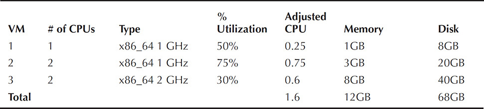
TABLE 5-1.    Sizing Information

Using this spreadsheet, you can then begin the design stage.

Example 2    In the example shown in Table 5-2, data has been collected for a half dozen very busy systems. This information will be used to analyze how much equipment is needed for the new installation. In this case, there are some holes in the data for new systems that don’t have an equivalent running system to collect data from.

TABLE 5-2.    Sizing Information

Using this spreadsheet, you can then begin the design stage.

Design

The design stage is where you choose the hardware for the VM Server system(s) and create a configuration. Sizing systems involves these components: the amount of memory, the number of CPUs, networking components, and the amount of disk space and storage performance required.

Sizing Memory    Because Oracle VM does not over-allocate memory, sizing memory is probably the easiest part of this exercise. Simply sum the memory required for each of the virtual machines to be supported and add an additional gigabyte for dom0. In the case of the preceding two examples, the required memory is pretty self-explanatory.

Sizing CPUs    Sizing CPUs is a little bit more challenging than sizing memory. This is mainly because CPUs are a shared resource and are always over-allocated. Over-allocating means it is common that more CPUs are allocated to the virtual machines than actually exist on the VM server system. Fully allocating CPUs to virtual machines is not feasible because they will not be fully utilized.

It is possible (and very probable) that virtual machines will utilize all of their allocated CPUs at one time or another, but it is very unlikely that they will run at that load for an extended period of time. This is why over-allocating CPU resources is possible. Because CPU resources are limited, if a one-to-one allocation of CPUs to virtual machines is used, the number of VM server CPUs would be much higher than really needed. The idea is to have as many as you need, but not to buy more than is necessary.

Sizing the Network    Sizing the network is another important component of sizing the VM server farm. The network is used for virtual machine network traffic as well as potentially for storage traffic (NFS). In addition, the network is used for live migration of virtual machines. The performance of the network is crucial in all of these tasks.

The network should be sized for peak utilization as well as for steady state operations. Peak utilization will occur during a live migration. A slow network could cause minutes or hours of additional migration time.

Sizing the Disks    Disk or I/O sizing has become much more difficult since most storage is virtualized now. That is, a disk or array is no longer allocated for a single purpose. Instead, pieces of the same array are allocated to many different purposes and potentially to different organizations and applications. Storage sizing is broken into two main components: sizing for capacity and sizing for performance.

Sizing for capacity is easy. In the example shown in Table 5-1, 68GB of storage is required. In the example in Table 5-2, 480GB of storage is required. That’s the easy part. The more difficult part is identifying the performance characteristics needed and sizing properly for them. If the I/O subsystem is undersized, the entire environment might suffer.

Unfortunately, sizing for performance involves extensive monitoring and data collection, which often are very difficult to do. What’s more, various storage subsystems provide additional features, such as caching and acceleration, that enhance performance. Each storage subsystem works differently and requires specific knowledge to be able to ascertain which features will benefit Oracle VM.

Capacity Planning

Capacity planning is the process of planning the capacity of the system in order to meet future requirements for increased workloads or adding more business systems. Capacity planning is different from sizing in that instead of dealing with a new system and a somewhat unknown workload, it directly involves the system currently being used, so more information is available. Capacity planning results in either adding more hardware (upgrading) or replacing the existing hardware with new hardware. Whether you’re upgrading or replacing the hardware, the capacity planning exercise requires the same steps as with sizing: data collection, analysis, and design.

Unlike traditional servers, Oracle VM provides a straightforward, almost seamless, upgrade path. If the VM server farm needs additional capacity, add a new VM server to the server pool. With the addition of the new VM server, you can migrate virtual machines to the new VM server seamlessly, thus spreading out the load to a new server. If a specific virtual machine needs additional capacity, you can easily add CPUs and memory (as long as they are available on the VM server).

In addition, the Oracle VM Server farm requires capacity planning not only for the VM servers, but also for the virtual machines themselves. Capacity planning for the Oracle VM Server farm involves monitoring both the Oracle VM Server itself and the individual virtual machines. As mentioned earlier in this section, the basic steps involved in capacity planning are similar to those involved in sizing: data collection, analysis, and design.

Data Collection

In the section on sizing, the focus was geared toward collecting data from individual servers with the goal of sizing a virtualized environment to host them. This section is geared toward collecting data from an already virtualized environment.

Data collection from a capacity planning standpoint is a little different from a sizing exercise. Here, you already have existing systems that hopefully have long-term monitoring enabled on them. Oracle Enterprise Manager (OEM) Cloud Control is an excellent product for monitoring virtualized environments for capacity planning purposes because of the ability to save years’ worth of data that you can then analyze.

In addition, tools such as the Xen Top command (xm top) will display resource utilization in an existing environment. An example of xm top is shown in Figure 5-3.

FIGURE 5-3.    xm top

If only the memory and number of virtual CPUs for the various domains are desired, you can acquire this with the command xm list, as shown in Figure 5-4.

FIGURE 5-4.    xm list

These statistics provide enough information to give you a good idea of how the individual virtual machines are performing and an idea of how things are currently running. Unfortunately, the xm top utility does not provide data in a tabular form that can be saved, unlike other OS utilities, such as sar.

Analysis

In the capacity planning analysis phase, you have to do more than in the analysis phase of the sizing exercise. When sizing, you design the system for the workload you have analyzed. When doing capacity planning, you analyze trends and determine future workloads. This involves extrapolation of existing data. Oracle Enterprise Manager (OEM) Cloud Control is an excellent tool for gathering long-term trend data for analysis.

Because capacity planning involves trend analysis and extrapolation, gathering long-term data is absolutely critical. Plot this data and extrapolate it for future workloads. In addition to gathering performance data, you need to gather business requirements. Business requirements should include any information related to future workloads as well as future applications and user counts, such as new call centers opening, the addition of personnel, and so on.

The final area of analysis involves how far into the future to look. Some companies prefer to plan hardware upgrades to handle workloads for the next two years; others want to handle the next three or four years. This is a business decision that must be included in the capacity planning calculations.

Design

The design stage varies based on whether the capacity planning is for individual virtual machines or for the Oracle VM Server. If the design is for a virtual machine, the modifications could be as simple as adding CPUs and/or more memory from the VM Manager. If the capacity planning activity is for the Oracle VM Server itself, you may be adding hardware, but, probably more likely, more Oracle VM Servers.

Virtualization provides much more flexibility than traditional servers. Rather than you having to move applications to new servers and/or shut down the server to add new CPU boards or memory, Oracle VM provides the ability to add a new Oracle VM Server to the server pool and then live migrate virtual machines to that new server seamlessly. This is one of the primary advantages of a virtualization environment.

Servers, CPUs, and Cores    You have multiple options when adding hardware to a virtualization environment. Adding more servers to a server pool by sharing the storage and joining the pool is an easy matter. Once you have determined that a new Oracle VM Server is needed, you can actually add it to the pool without incurring downtime from the pool. Simply add the server to the pool and configure load balancing and/or HA, and the rest is easy.

A less costly approach is to add resources to an existing server. You can often do this by adding CPUs with or without multiple cores. There is now an abundance of CPUs with multiple cores—anywhere from two to eight. Multiple-core systems came about as a result the chipmakers’ ability to add more and more components to a single chip.

A core is a CPU within a CPU. As integrated circuit density has increased, we now have the ability to add more compute power to the CPU by essentially creating multiple CPUs within the CPU chip. The local terminology for the CPU chip is a socket, whereas the individual compute engines within the chip are referred to as the cores.

The multiple-core CPU is an evolution of CPU technology. In the early days of the PC, the Intel/AMD architecture had a single core and appeared to the OS as a single CPU. PC vendors eventually developed multiprocessor systems that enabled more capacity within the same server. Later technology was known as hyperthreading or hyperthreaded CPU. This appeared to the PC as an additional CPU, but, in reality, hyperthreading was a method of taking advantage of CPU instruction cycles that might otherwise be wasted. Even though the OS thought that the hyperthreaded CPU was an additional CPU, it really only provided an additional 30 to 50 percent more performance.

The multiple-core CPU is actually an additional CPU built into the die of the chip. So the chip itself has multiple “CPUs” built in. These CPU chips also include the multiprocessor technology needed to maintain multiple CPUs and manage memory access between the chip and the RAM. Some designs even include a memory controller on the chip.

In addition to the multicore features, hardware acceleration for virtualization has been introduced to allow virtual machines to run at near native CPU speed. This has helped make virtualization very economical.

Regardless of whether additional CPUs/cores or entire VM servers are added to increase the VM server farm capacity, planning ahead is important. Planning for additional hardware when the system is out of capacity is too late. At that point, users will already be complaining.

Storage    Storage is fairly easy to plan for from a capacity standpoint but is often difficult to plan for from a performance standpoint. This is because storage administration is often not done by the same personnel who manage the servers and the virtual environment. In addition, there are many factors to consider, such as I/O subsystem cache, storage channels (such as fiber channel switches), and storage virtualization itself.

Storage-size capacity planning is best accomplished by keeping long-term monitoring data about the size and usage of your storage system. It is impossible to perform capacity planning tasks by looking at a single data point. To project future growth, you have to have data regarding past performance. Tools such as OEM Cloud Control can assist with this by monitoring both the space usage of the individual virtual machines and the VM Server itself. Because Oracle VM storage uses OCFS2, obtaining space information is not difficult. If no tools are available, it is easy to create a crontab script to collect space information on a regular basis. This will provide valuable information for future capacity planning.

Summary

A lack of proper planning can often lead to a poorly performing system. Through proper sizing, the right hardware can be allocated for the right job. This chapter provided information on how to perform sizing and capacity planning for the Oracle VM Server farm. Included was some information on how to monitor the performance of the VM server farm. Performance monitoring is covered throughout this book as well.

In the next chapter, you will learn how to install the Oracle VM Server. In later chapters, you will learn how to install and configure the Oracle VM Manager and OEM Cloud Control plug-in for Oracle VM.