Search in book...
Toggle Font Controls
Create new playlist

Name your new playlist

Playlist description (optional)
Sign In

Email address

Password

Forgot Password?

or

Continue with Facebook

Continue with Google
Sign Up

Full Name

Email address

Confirm Email Address

Password

or

Continue with Facebook

Continue with Google

Principal component analysis (PCA) is a statistical procedure that uses an orthogonal transformation to convert a set of observations of possibly correlated variables into a set of values of linearly uncorrelated variables called principal components. The number of principal components is less than or equal to the number of original variables. This transformation is defined in such a way that the first principal component has the largest possible variance (i.e., accounts for as much of the variability in the data as possible), and each succeeding component in turn has the highest variance possible under the constraint that it is orthogonal to the preceding components. The resulting vectors are an uncorrelated orthogonal basis set. The principal components are orthogonal because they are the eigenvectors of the covariance matrix, which is symmetric. PCA is sensitive to the relative scaling of the original variables.

12.2 Description of the Problem

Given data {x₁, …, x_N} where each element x_j has m attributes {a_j1, …, a_jm} and j = 1, …, N. While applying a machine learning classification or clustering algorithm, it is not expected from all the features (attributes) to have valuable contributions to the resulting classification or clustering model. The attributes with the least contributions do act as noise, and reducing them from the data will result in a more effective classification or clustering model.

The PCA is a multivariate statistical technique aiming at extracting the features that represent most of the information in the given data and eliminating the least features with least information. Therefore, the main purpose of using the PCA is to reduce the dimensionality of the data without seriously affecting the structure of the data.

When collecting real data, usually the random variables that represent the data attributes are expected to be highly correlated. The correlations between these random variables can always be seen in the covariance matrix. The variances of the random variables are found in the diagonal of the covariance matrix. The sum of the variances (diagonal elements of the covariance matrix) gives the overall variability. In Table 12.1, we show the covariance matrix of the “ecoli” data consisting of seven attributes.

The PCA works to replace the original random variables with other sets of orthonormal set of vectors called the principal components. The first principal component is desired to pass as much closer as possible to data points, and the projection of the data into the space spanned by the first component is the best projection over spaces spanned by other vectors in one dimension. The second principal component is orthogonal to the first principal component and the plain spanned by it together with the first component is the closest plane to the data. The third, fourth, and other such components feature at the same logic. In the new space with the same dimension as the original space, the covariance matrix is a diagonal matrix, and preserves the total variability of the original covariance matrix.

Table 12.1 The Covariance Matrix of the Ecoli Dataset, with Seven Random Variables Representing the Seven Data Attributes

In Figure 12.1a, we generated two-dimensional (2D) random data. Then, we used the PCA to project the 2D data into the first component (Figure 12.1b). We show the projected data in the figure.

12.3 The Idea behind the PCA

Given an m-dimensional data D of the form:

D = [\begin{matrix} x_{1} \\ x_{2} \\ ⋮ \\ x_{N} \end{matrix}] = [\begin{matrix} a_{11} & a_{12} & \dots & a_{1 m} \\ a_{21} & a_{22} & \dots & a_{2 m} \\ ⋮ & ⋮ & ⋱ & ⋮ \\ a_{N 1} & a_{N 2} & \dots & a_{M m} \end{matrix}]

$D = [\begin{matrix} x_{1} \\ x_{2} \\ ⋮ \\ x_{N} \end{matrix}] = [\begin{matrix} a_{11} & a_{12} & \dots & a_{1 m} \\ a_{21} & a_{22} & \dots & a_{2 m} \\ ⋮ & ⋮ & ⋱ & ⋮ \\ a_{N 1} & a_{N 2} & \dots & a_{M m} \end{matrix}]$

The data D can be visualized by Figure 12.2. Hence, each data element x_j is represented by an m-dimensional row vector.

Figure 12.1 (a) The original two-dimensional data in the feature space and (b) the reduced data in one-dimensional space.

Figure 12.2 The shape of a dataset consisting of N feature vectors, each has m attributes.

The main purpose of using the PCA is to reduce the high-dimensional data with a dimension m into a lower dimensional data of dimension k, where k ≤ m. The basis elements of the reduced space V constitute an orthonormal set. That is, if {v₁, v₂, …, v_k} is the basis of V, then:

v_{i}^{T} \cdot v_{j} = {\begin{matrix} 1, & j = i \\ 0, & j \neq i \end{matrix}

$v_{i}^{T} \cdot v_{j} = {\begin{matrix} 1, & j = i \\ 0, & j \neq i \end{matrix}$

The singular value decomposition (SVD) plays the main role in computing the basis elements {v₁, …, v_k}.

12.3.1 The SVD and Dimensionality Reduction

Suppose that C is the covariance matrix that is extracted from a given dataset D. The elements of the covariance matrix are the covariances between the random variables representing the data attributes (or features). The variance of the random variables lies in the diagonal of C, and their sum is the total variability. Generally, the SVD works to express matrix C as a product of three matrices: U, ∑, and V. Because matrix C is an m × m matrix, the SVD components of matrix C are given by

C = U∑V^T

where:

U and V are orthogonal m × m matrices

∑ is an m × m diagonal matrix

The diagonal elements of ∑ are the eigenvalues of the covariance matrix C, ordered according to their magnitudes from bigger to smaller. The columns of U (or V) are the eigenvectors of matrix C that correspond to the eigenvalues of C.

By factoring matrix C into its SVD components, we would be rewarded with three benefits:

The SVD identifies the dimensions along which data points exhibit the most variation, and order the new dimensions accordingly. The total variation exhibited by the data is equal to the sum of all eigenvalues, which are the diagonal elements of the matrix ∑ and the variance of the jth principal component is the jth eigenvalue.
Replace the correlated variables of the original data by a set of uncorrelated ones that are better exposed to the various relationships among the original data items. The columns of matrix U, which are the eigenvectors of C, define the principal components, which act as the new axes for the new space.
As a result of benefit (2), the SVD finds the best approximation of the original data points using fewer dimensions. Reducing the dimension is done through selecting the first k principal components, which are the columns of matrix U.

12.4 PCA Implementation

The steps to implement the PCA are as follows:

Step 1: Compute the mean of the data as follows:

Let

\bar{x} = [\begin{matrix} \bar{a_{1}} & \bar{a_{2}} & \dots & \bar{a_{m}} \end{matrix}] = \frac{1}{N} \sum_{j = 1}^{N} x_{j}

$\bar{x} = [\begin{matrix} \bar{a_{1}} & \bar{a_{2}} & \dots & \bar{a_{m}} \end{matrix}] = \frac{1}{N} \sum_{j = 1}^{N} x_{j}$

Step 2: Normalize the data by subtracting the mean value $\bar{x}$ $\bar{x}$ , from all the instances x_i giving the adjusted mean vectors $x_{i} - \bar{x}$ $x_{i} - \bar{x}$ . Therefore, the normalized data $\bar{D}$ $\bar{D}$ , is given by

\bar{D} = [\begin{matrix} x_{1} - \bar{x} \\ x_{2} - \bar{x} \\ ⋮ \\ x_{N} - \bar{x} \end{matrix}]

$\bar{D} = [\begin{matrix} x_{1} - \bar{x} \\ x_{2} - \bar{x} \\ ⋮ \\ x_{N} - \bar{x} \end{matrix}]$

The values $x_{i} - \bar{x}$ $x_{i} - \bar{x}$ are the deviations of the data from its mean; hence, the adjusted mean features are centered at zero.

Step 3: Construct the covariance matrix $COV (\bar{D}) ∊ R^{m \times m}$ $COV (\bar{D}) ∊ R^{m \times m}$ from $\bar{D}$ $\bar{D}$ as follows:

(COV (\bar{D}))_{ij} = \frac{1}{N} \sum_{n = 1}^{N} (x_{ni} - {\bar{a}}_{i}) \cdot (x_{nj} - {\bar{a}}_{j})

$(COV (\bar{D}))_{ij} = \frac{1}{N} \sum_{n = 1}^{N} (x_{ni} - {\bar{a}}_{i}) \cdot (x_{nj} - {\bar{a}}_{j})$

Step 4: Let {λ₁, λ₂,…,λ_m} be the set of eigenvalues of the covariance matrix COV( $\bar{D}$ $\bar{D}$ ), in a way that |λ₁|≥|λ₂|≥…≥|λ_m| and {v₁, v₂, …, v_m} are the corresponding set of eigenvectors. The k vectors v₁, v₂, …, v_k represent the first k principal components.

Step 5: Construct the following matrix:

F = [v₁ v₂ ⋯ v_k] ∊ R^m×k

The reduced data in k-dimensions will be

{\bar{D}}_{reduced} = \bar{D} \cdot F ∊ R^{N \times k}

${\bar{D}}_{reduced} = \bar{D} \cdot F ∊ R^{N \times k}$

12.4.1 Number of Principal Components to Choose

When applying the PCA, the variances of the random variables are represented by the eigenvalues of the covariance matrix that are located at the main diagonal of matrix ∑. In matrix ∑ the eigenvalues are sorted according to their magnitudes, from bigger to smaller. That means, the principal component with bigger variance comes first. Let S ∊ R^m be the vector of the diagonal elements of ∑. The variance retained by choosing the first k principal components is given by

Table 12.2 Variances of the Seven Principal Components of Ecoli Data

\frac{\sum_{j = 1}^{k} S_{j}}{\sum_{j = 1}^{m} S_{j}}

$\frac{\sum_{j = 1}^{k} S_{j}}{\sum_{j = 1}^{m} S_{j}}$

We applied the PCA algorithm to the “ecoli” data, and the variance retained by the first k principal components are explained in Table 12.2.

This means that if we select only the first principal component, then we can retain only 51.6% of the variance. If we select the first two principal components, then 76% of the variance will be retained, and so on.

By knowing this, we can determine how many principal components to select. For example, if we need to retain 90% at least of the variance, then we shall choose the first four principal components, if we need 99% of the variance, then we shall select the first six principal components.

12.4.2 Data Reconstruction Error

If ${\tilde{x}}_{i} = x_{i} - \bar{x} ∊ \bar{D}$ ${\tilde{x}}_{i} = x_{i} - \bar{x} ∊ \bar{D}$ , then $z_{i} = {\tilde{x}}_{i} \cdot F ∊ R^{k}$ $z_{i} = {\tilde{x}}_{i} \cdot F ∊ R^{k}$ is the projection of ${\tilde{x}}_{i}$ ${\tilde{x}}_{i}$ in the new linear space spanned by the orthonormal basis vectors {v₁, v₂, …, v_k}. Moving from R^m to R^k is reversible and one can reconstruct ${\overset{⌃}{x}}_{i}$ ${\overset{⌃}{x}}_{i}$ , which is an approximation to ${\tilde{x}}_{i}$ ${\tilde{x}}_{i}$ , where:

Table 12.3 Reconstruction Errors Obtained by Applying PCA with k Principal Components

{\overset{⌃}{x}}_{i} = z_{i} \cdot F^{T} ∊ R^{m}

${\overset{⌃}{x}}_{i} = z_{i} \cdot F^{T} ∊ R^{m}$

The error associated with the data reconstruction Error_Rec is given by

{Error}_{Rec} = \sum_{i = 1}^{N} | | {\tilde{x}}_{i} - {\overset{⌃}{x}}_{i} | |^{2}

${Error}_{Rec} = \sum_{i = 1}^{N} | | {\tilde{x}}_{i} - {\overset{⌃}{x}}_{i} | |^{2}$

The reconstruction errors obtained by applying the PCA with k principal components are explained in the Table 12.3.

12.5 The Following MATLAB^® Code Applies the PCA

function [Dred, Drec, Error] = PCAReduction(D, k)
% D is a dataset, consisting of N instances (rows)
and m features (columns)
% k is the new data dimension, where 0 <= k <= m
[N, m] = size(D)  ; % Number of data instances N and
number of features is m
mu = mean(D)  ;    % mean of data set --> mu
 
Db = zeros(size(D))  ;  % Db is the mean adjusted
dataset
for j = 1 : N
    Db(j, :) = D(j, :) - mu ;
    % subtracting the mean from the N data
instances
end
 
C = zeros(m) ; % C is the covariance matrix
for i = 1 : m
    for j = 1 : m
        C(i, j) = 0 ;
        for n = 1 : N
            C(i, j) = C(i, j) + Db(n, i)*Db(n, j)/N ;
        end
    end
end
 
[U, S, V] = svd(C) ; % Applying the SVD to the
covariance matrix
F = V(:, 1:k) ;      % F is the matrix with the
first k components
Dred = Db*F ; % Generating the reduced data
Drec = Dred*F’ ; % Reconstructing the mean adjusted
data in m-dimensions
 
for j = 1 : N
    Drec(j, :) = Drec(j, :) + mu ; % Reconstructing
the original data
end
Error = norm(Drec-D, 2)^2 % Computing the error

We applied the above algorithm to the Iris dataset with k = 2. In Figure 12.3, we show the plot of the reduced data (which is 2D).

We also plotted the data in a three-dimensional reduced space in Figure 12.4.

Figure 12.3 Two-dimensional reduced data.

Figure 12.4 Three-dimensional reduced space.

12.6 Principal Component Methods in Weka

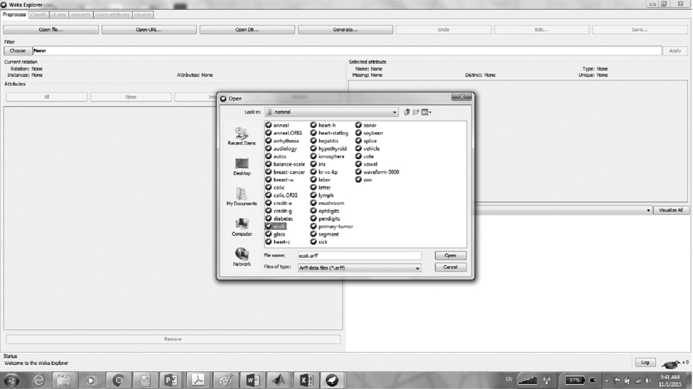
Open Weka and from the Weka explorer open the ecoli. arff file using the Open File button. The file ecoli.arff contains the ecoli dataset.
From the preprocess tab, choose Filter–>unsupervised–> attribute–>principal component.
Press the apply button to enable the principal component filter to work.
The statistics of the new resulting features, including the maximum and minimum values, the mean, and the standard deviation, can be seen.
You can notice that Weka has already reduced the number of features from seven to six. That is, the dimension is reduced by one.
However, Weka still enables the users to do further reductions if needed, where the standard deviation can be used to determine which features to eliminate and which features to keep. The smaller the standard deviation, higher will be the probability of that feature being eliminated.

12.7 Example: Polymorphic Worms Detection Using PCA

12.7.1 Introduction

Internet worms pose a major threat to the Internet infrastructure security, and their destruction causes loss of millions of dollars. Therefore, the networks must be protected as much as possible to avoid losses. This thesis proposes an accurate system for signature generation for Zero-day polymorphic worms.

This example consists of two parts.

In part one, polymorphic worm instances are collected by designing a novel double-honeynet system, which is able to detect new worms that have not been seen before. Unlimited honeynet outbound connections are introduced to collect all polymorphic worm instances. Therefore, this system produces accurate worm signatures. This part is out of the scope of this example.

In part two, signatures are generated for the polymorphic worms that are collected by the double-honeynet system. Both a Modified Knuth–Morris–Pratt (MKMP) algorithm, which is string matching based, and a modified principal component analysis (MPCA), which is statistics based, are used. The MKMP algorithm compares the polymorphic worms’ substrings to find the multiple invariant substrings that are shared between all polymorphic worm instances and uses them as signatures. The MPCA determines the most significant substrings that are shared between polymorphic worm instances and uses them as signatures [1].

12.7.2 SEA, MKMP, and PCA

This section discusses two parts. The first part presents our proposed substring exaction algorithm (SEA), MKMP algorithm, and MPCA, which are used to generate worm signatures from a collection of worm variants captured by our double-honeynet system [1].

To explain how our proposed algorithms generate signatures for polymorphic worms, we assume that we have a polymorphic worm A, which has n instances (A₁, A₂, …, A_n). Generating a signature for polymorphic worm A involves two steps:

■ First, we generate the signature itself.
■ Second, we test the quality of the generated signature by using a mixed traffic (new variants of polymorphic worm A, and normal traffic).

Before stating the details of our contributions and the subsequent analysis part, we briefly mention an introduction about string matching search method and the original Knuth–Morris–Pratt (KMP) algorithm to give a clear picture of the subject topic.

The second part discusses the implementation results of our proposed algorithms.

12.7.3 Overview and Motivation for Using String Matching

In this and the following sections, we will describe SEA, MKMP algorithm, and modified PCA to highlight our contributions.

String matching [2] is an important subject in the wider domain of text processing. String matching algorithms are basic components used in implementations of practical software used in most of the available operating systems. Moreover, they emphasize programming methods that serve as paradigms in other fields of computer science (system or software design). Finally, they also play an important role in theoretical computer science by providing challenging problems.

String matching generally consists of finding a substring (called a pattern) within another string (called the text). The pattern is generally denoted as

x = x[0. .m-1]

Whose length is m and the text is generally denoted as

y = y[0. .n-1]

whose length is n. Both the strings pattern and text are built over a finite set of characters, which is called the alphabet, and is denoted by ∑ whose size is denoted by σ.

The string matching algorithm plays an important role in network intrusion detection systems (IDSs), which can detect malicious attacks and protect the network systems. In fact, at the heart of almost every modern IDS, there is a string matching algorithm. This is a very crucial technique because it allows detection systems to base their actions on the content that is actually flowing to a machine. From a vast number of packets, the string identifies those packets that contain data, matching the fingerprint of a known attack. Essentially, the string matching algorithm compares the set of strings in the ruleset with the data seen in the packets, which flow across the network.

Our work uses SEA and MKMP algorithm (which are based on string matching algorithms) to generate signatures for polymorphic worm attacks. The SEA aims at extracting substrings from polymorphic worm, whereas the MKMP algorithm aims to find out multiple invariant substrings that are shared between polymorphic worm instances and to use them as signatures.

12.7.4 The KMP Algorithm

The KMP string searching algorithm [1] searches for occurrences of a word, W, within a main text string, S, by employing the observation that when a mismatch occurs, the word itself embodies sufficient information to determine where the next match could begin, thus bypassing reexamination of previously matched characters [1].

Let us take an example to illustrate how the algorithm works. To illustrate the algorithm’s working method, we will go through a sample run (relatively artificial) of the algorithm. At any given time, the algorithm is in a state determined by two integers, m and i. The integer m denotes the position within S, which is the beginning of a prospective match for W, and i denotes the index in W denoting the character currently under consideration. This is depicted at the start of the run as follows:

m: 01234567890123456789012
S: ABC ABCDAB ABCDABCDABDE
W: ABCDABD
i: 0123456

We proceed by comparing successive characters of W to parallel positional characters of S, moving from one to the next if they match. However, in the fourth step in our noted case, we get that S[3] is a space and W[3] is equal to the character D (i.e., W[3] = “D”), which is a mismatch. Rather than beginning to search again at the position S [1], we note that no A occurs between positions 0 and 3 in S except at 0. Hence, having checked all those characters previously, we know that there is no chance of finding the beginning of a match if we check them again. Therefore, we simply move on to the next character, setting m = 4 and i = 0.

m: 01234567890123456789012
S: ABC ABCDAB ABCDABCDABDE
W:     ABCDABD
i:     0123456

We quickly obtain a nearly complete match “ABCDAB,” but when at W[6] (S[10]), we again have a discrepancy. However, just prior to the end of the current partial match, we passed an “AB” which could be the beginning of a new match, so we must take this into consideration. As we already know that these characters match the two characters prior to the current position, we need not check them again; we simply reset m = 8, i = 2, and continue matching the current character. Thus, not only do we omit previously matched characters of S but also previously matched characters of W.

m: 01234567890123456789012
S: ABC ABCDAB ABCDABCDABDE
W:         ABCDABD
i:         0123456

We continue with the same method of matching till we match the word W.

12.7.5 Proposed SEA

In this subsection, we show how our proposed SEA is used to extract substrings from one of the polymorphic worm variants that are collected by the double-honeynet system.

This subsection and Section 12.7.6 show the signature generation process for polymorphic worm A using the SEA and the MKMP algorithm.

Let us assume that we have a polymorphic worm A, that has n instances (A₁, …, A_n) and A_i has length M_i, for i = 1, …, n. Assume that A₁ is selected to be the instance from which we extract substrings and the A₁ string contains a₁ a₂ a₃ … a_m1. Let X be the minimum length of a substring that we are going to extract from A₁. The first substring from A₁ with length X, is (a₁ a₂ … a_x). Then, we shift one position to the right to extract a new substring, which will be (a₂ a₃ … a_x+1). Continuing this way, the last substring from A₁ will be (a_m1−X + 1 … a_m1). In general, for instance, A_i has length equal to M, and if a minimum length of the substring that we are going to extract from A₁ equals to X, then the total number of substrings (TNSs) that will be extracted from A_i could be obtained by the following equation [1]:

TNS (Ai) = M-X+1

The next step is to increase X by one and start new substrings extraction from the beginning of A₁. The first substring will be (a₁ a₂ … a_x+1). The substrings extraction will continue satisfying this condition: X < M.

Figure 12.5 and Table 12.4 show all substrings extraction possibilities using the proposed SEA from the string ZYXCBA, assuming the minimum length of X is equal to three.

The output of the SEA will be used by both the MKMP algorithm and the modified PCA method. The MKMP algorithm uses the substrings extracted by the SEA to search the occurrences of each substring in the remaining of the instances (A₂, A₃, …, A_n). The substrings that occur in all the remaining instances will be considered as worm signature. To clarify some of the points noted here, we will present the details of the MKMP algorithm in Section 12.7.6 [1].

Figure 12.5 Extraction substrings.

Table 12.4 Substrings Extraction

12.7.6 An MKMP Algorithm

Here, we describe our modification to the KMP algorithm. As mentioned in Section 12.7.4, the KMP algorithm searches for occurrences of W (word) within S (text string). Our modification of the KMP algorithm is to search for occurrence of different words (W₁, W₂, …, W_n) within string text S. For example, say we have a polymorphic worm A, with n instances (A₁, A₂, …, A_n). Let us select A₁ to be the instance from which we would extract substrings. If nine substrings are extracted from A₁, each substring will be W_i, for i = 1 to 9. This means that A₁ has nine words (W₁, W₂, …, W₉), whereas the remaining instances (A₂, A₃, …, A_n) are considered as S text string [1].

Considering the above example, the MKMP algorithm searches the occurrences of W₁ in the remaining instances of S (A₂, A₃, …, A_n). If W₁ occurs in all remaining instances of S, then we consider it as signature, otherwise we ignore it. The other words (W₂, W₃, …, W₉) are similarly dealt with. For example, if W₁, W₅, W₆, and W₉ occur in all remaining instances of S, then W₁, W₅, W₆, and W₉ are considered a signature of the polymorphic worm A.

12.7.6.1 Testing the Quality of the Generated Signature for Polymorphic Worm A

We test the quality of the generated signature for polymorphic worm A by using a mixed traffic (new variants of polymorphic worm A and normal traffic, i.e., innocuous packets). The new variants of polymorphic worm A are not the same variants that are used to generate the signature. Let us assume that our system received a packet P (where P contains either malicious or innocuous data). The MKMP algorithm compares P payload against the generated signature to determine whether P is a new variant of polymorphic worm A or not. The MKMP algorithm considers P as a new variant of the polymorphic worm A, if all the substrings of the generated signature appear in P.

12.7.7 A Modified Principal Component Analysis

12.7.7.1 Our Contributions in the PCA

In Sections 12.7.7.1 and 12.7.7.2, we show the signature generation process for polymorphic worm A using an MPCA.

In our work, instead of applying PCA directly, we have made appropriate modifications to fit it with our mechanism. Our contribution in the PCA method is in combining the PCA (i.e., extend) with the proposed SEA to get more accurate and relatively faster signatures for polymorphic worms. The extended method (SEA and PCA) is termed MPCA. We have previously mentioned that the polymorphic worm evades the IDSs by changing its payload in every infection attempts; however, there are some invariant substrings that will remain fixed (i.e., some substrings will not change) in all polymorphic worm variants, so the SEA extracts substrings from the polymorphic worm in a good way (i.e., it will extract all the possibilities of substrings from a polymorphic worm variant, which contain worm signature) that helps us to get accurate signatures. After the SEA extracts the substrings, it will pass those to the PCA, thus, easing the heavy burden to the PCA in terms of time (i.e., the PCA directly will start by determining the frequency Count of each substring in rest of the instances without doing substring extraction process).

After the PCA receives the substrings from SEA, it will determine the frequency count of each substring in the remaining instances (A₂, A₃, …, A_n). Finally, the PCA will determine the most significant data on the polymorphic worm instances and use them as signature []. We present the details in Section 12.7.7.1.1.

12.7.7.1.1 Determination of Frequency Counts

Here, we determine the frequency count of each substring S_i (A₁ substrings), in each of the remaining instances (A₂, …, A_n). Then, we apply the PCA on the frequency count data to reduce the dimension and get the most significant data.

12.7.7.1.2 Using PCA to Determine the Most Significant Data on Polymorphic Worm Instances

The methodology of employing PCA to the given problem is outlined below.

Let F_i denote the vector of frequencies (F_i1, …, F_iN) of the substring S_i in the instances (A₁, …, A_n), i = 1, …, L.

We construct the frequency matrix F by letting F_i be the ith row of F, provided that F_i is not the zero vector [3].

F = (\begin{matrix} f_{11} & \dots & f_{1 N} \\ ⋮ & ⋱ & ⋮ \\ f_{L 1} & \dots & f_{L N} \end{matrix})

$F = (\begin{matrix} f_{11} & \dots & f_{1 N} \\ ⋮ & ⋱ & ⋮ \\ f_{L 1} & \dots & f_{L N} \end{matrix})$

12.7.7.1.3 Normalization of Data

The normalization of the data is applied by normalizing the data in each row of the matrix F, yielding a matrix D (L × N).

D = (\begin{matrix} d_{11} & \dots & d_{1 N} \\ ⋮ & ⋱ & ⋮ \\ d_{L 1} & \dots & d_{L N} \end{matrix})

$D = (\begin{matrix} d_{11} & \dots & d_{1 N} \\ ⋮ & ⋱ & ⋮ \\ d_{L 1} & \dots & d_{L N} \end{matrix})$

d_{i k} \leftarrow \frac{f_{i k}}{\sum_{j = 1}^{N} f_{i j}}

$d_{i k} \leftarrow \frac{f_{i k}}{\sum_{j = 1}^{N} f_{i j}}$

12.7.7.1.4 Mean Adjusted Data

To get the data adjusted around zero mean, we use the following formula:

\begin{matrix} g_{i k} \leftarrow d_{i k} - {\bar{d}}_{i} & \forall i, k \end{matrix}

$\begin{matrix} g_{i k} \leftarrow d_{i k} - {\bar{d}}_{i} & \forall i, k \end{matrix}$

where $\begin{matrix} {\bar{d}}_{i} \end{matrix}$ $\begin{matrix} {\bar{d}}_{i} \end{matrix}$ is the mean of the ith vector

= \frac{1}{N} \sum_{j = 1}^{N} d_{i j}

$= \frac{1}{N} \sum_{j = 1}^{N} d_{i j}$

The data adjust matrix G is given by

G = (\begin{matrix} g_{11} & \dots & g_{1 N} \\ ⋮ & ⋱ & ⋮ \\ g_{L 1} & \dots & g_{L N} \end{matrix})

$G = (\begin{matrix} g_{11} & \dots & g_{1 N} \\ ⋮ & ⋱ & ⋮ \\ g_{L 1} & \dots & g_{L N} \end{matrix})$

12.7.7.1.5 Evaluation of the Covariance Matrix

Let g_i denote the ith row of G, then the covariance between any two vectors g_i and g_j is given by

Cov (g_{i}, g_{j}) = C_{i j} - \frac{\sum_{k = 1}^{L} (d_{i k} - {\bar{d}}_{i}) (d_{j k} - {\bar{d}}_{j})}{N - 1}

$Cov (g_{i}, g_{j}) = C_{i j} - \frac{\sum_{k = 1}^{L} (d_{i k} - {\bar{d}}_{i}) (d_{j k} - {\bar{d}}_{j})}{N - 1}$

Then the covariance matrix C (N × N) is given by

C = (\begin{matrix} C_{11} & \dots & C_{1 N} \\ ⋮ & ⋱ & ⋮ \\ C_{N 1} & \dots & C_{N N} \end{matrix})

$C = (\begin{matrix} C_{11} & \dots & C_{1 N} \\ ⋮ & ⋱ & ⋮ \\ C_{N 1} & \dots & C_{N N} \end{matrix})$

12.7.7.1.6 Eigenvalue Evaluation

Evaluate the eigenvalues of the matrix C from its characteristic polynomial |C − λI| = 0, and then compute the corresponding eigenvectors.

12.7.7.1.7 Principal Component Evaluation

Let L₁, L₂, …, L_N be the eigenvalues of the matrix C obtained by solving the characteristic equation |C − λI| = 0. If necessary, resort the eigenvalues of C in a descending order such that |L₁|>=…>=|L_N|. Let V₁, V₂, …, V_N be the eigenvectors of matrix C corresponding to the eigenvalues L₁, L₂, …, L_N. The k principal components are given by V₁, V₂, …, V_K, where K<=N [3].

12.7.7.1.8 Projection of Data Adjust along the Principal Component

Let V be the matrix that has the k principal components as its columns. That is,

V = [V₁, V₂, …, V_k]

Then, feature descriptor (FD) is obtained from the following equation:

Feature descriptor = V^T × F

To determine the threshold of polymorphic worm A, we use a distance function (Euclidean distance) to evaluate the maximum distance between the rows of F and the rows of FD. The maximum distance R works as a threshold [3].

12.7.7.2 Testing the Quality of Generated Signature for Polymorphic Worm A

In Section 12.7.7.1, we calculated the FD and the threshold for polymorphic worm A. Here, we test the quality of generated signature for polymorphic worm A by using a mixed traffic (new variants of polymorphic worm and normal traffic, i.e., innocuous packets), the new variants of polymorphic worm A are not the same variants that are used to generate the signature.

Let us assume that our system received a packet P (where P contains either malicious or innocuous data). The MPCA performs the following steps to determine whether P is a new variant of polymorphic worm A or not [1]:

■ Determine frequencies of the substrings of W array in P (W array contains extracted substrings of A₁, as mentioned earlier). This will produce a frequency matrix F₁.
■ Calculate the distance between the polymorphic worm FD and F₁ using Euclidean distance. This will produce a distance matrix D₁.
■ Compare the distances in D₁ to the threshold R of polymorphic worm A. If any <= the threshold, classify P as a new variant of polymorphic worm A.

12.7.7.3 Clustering Method for Different Types of Polymorphic Worms

When our network receives different types of polymorphic worms (mixed polymorphic worms), we must first separate them into clusters and then generate signatures to each cluster as the same as in Sections 12.7.7.1 and 12.7.7.2. To perform the clustering, we use Euclidean distance, which is the most familiar distance metric. Euclidean distance is frequently used as a measure of similarity in the nearest neighbor method []. Let X = (X₁, X₂, …, X_p)′ and Y = (Y₁, Y₂, …, Y_p)′. The Euclidean distance between X and Y is as follows [1]:

d (X, Y) = \sqrt{(X - Y)' (X - Y)}

$d (X, Y) = \sqrt{(X - Y)' (X - Y)}$

12.7.8 Signature Generation Algorithms Pseudo-Codes

Here, we describe the signature generation algorithms pseudo-codes. These algorithms were discussed above, and as mentioned there, generating a signature for polymorphic worm A involves two steps:

■ First, we generate the signature itself.
■ Second, we test the quality of the generated signature by using a mixed traffic (new variants of polymorphic worm A and normal traffic).

12.7.8.1 Signature Generation Process

This section shows the pseudo-codes for generating a signature for polymorphic worm A using SEA, MKMPA, and MPCA.

12.7.8.1.1 SEA Pseudo-Code

In the following, we describe the pseudo-code of the SEA, which was discussed above. The goal of SEA is to extract substrings from the first instance of polymorphic worm A and then to put them in an array W [1].

SEA pseudo-code:

     1. Function SubstringExtraction:
     2. Input (a file A1: First instance of polymorphic
        worm A, x: minimum substring length)
     3. Output: (W: array of substrings of A1 with a
        minimum substring length x)
     4. Define variables:
        Integer M : Length of file A1
        Integer X: Maximum substring length
        Integer z: (x<=z<=X) takes the lengths x to X
        Integer Tz: Total number of substrings of
        file A1 with a substring length z
        Integer position: the position of the first
        character of a substring of A1 with length z.
        Array of characters S: a substring of A1 with
        length z
     5. X= M-1
     6.   For  z := x to X Do
     7.        Set Tz = M-z+1
     8.         Set position = 0
     9.                While  position <= Tz
    10.                        S = A1 (position) to
                               A1(position+z-1)
    11.                        Append (W, S)
    12.                        position←position +1
    13.                EndWhile
        EndFor
    14. Return W.

12.7.8.1.2 MKMP Algorithm Pseudo-Code

In the following, we present the pseudo-code for the MKMP algorithm. Consider the example mentioned in Section 12.7.2 that we have a polymorphic worm with n instances (A₁, A₂, …, A_n). We select A₁ to be the instance from which we extract substrings. If G substrings are extracted from A₁, each substring will be equal to W_i for i = 1 to G. That means A₁ has G words (W₁, W₂, …, W_G), whereas the remaining instances (A₂, A₃, …, A_n) are considered as S text string [1].

The MKMP algorithm contains two functions:

“Kmpfound” function

The Kmpfound function is an MKMP algorithm, which receives a word w from W array (W₁, W₂, …, W_G) and a File S (one file of the remaining instances A₂, …, A_n) and determines whether w can be found in S or not.
“Signaturefile” Function

The Signaturefile function is combined together with the above function to get out the words (W₁, W₂, …, W_G) that appear in all of the remaining instances (A₂, …, A_n), and use them as worm signature.

The MKMP algorithm has two inputs:

■ The first input is the substring of the W array (the output of the SEA).
■ The second input is the remaining instances (A₂, …, A_n)

The goal of the MKMP algorithm is to determine which substrings of W array appear in all remaining instances (A₂, …, A_n), and to use them as a suspected worm signature.

MKMP algorithm pseudo-code: “kmpfound” function

    1. Function kmpfound
    2. Inputs:
       S: an instance of polymorphic worm A (A2, ... , An)
       w: a word from file W to be searched in file
       S /* W is the output of the SEA */
    3. Output:
       a boolean value (true if w is found in S, and
       false otherwise)
    4. Define variables:
       an integer, m ← 0 (the beginning of the
       current match in S)
       an integer, i ← 0 (the position of the
       current character in w)
       an array of integers, T (the table, computed
       elsewhere)
    5. while m+i is less than the length of S, do:
    6.     if w[i] = S[m + i],
    7.             if i equals the (length of w)-1,
    8.                     return true
    9.             let i ← i + 1
   10.     Otherwise,
   11.             let m ← m + i - T[i],
   12.             if T[i] is greater than -1,
   13.                      let i ← T[i]
   14.                    else
   15.                      let i ← 0
   16.     Return false.

MKMP algorithm pseudo-code: “SignatureFile” function

    1. Function SignatureFile
    2. Inputs:
       W: Array of substrings of A1
       A2, ..., An: Instances of worm A
    3. Output:
              SigFile : Array of substrings of A1
              found in the rest instances (A2, ..., An)
              (Signature file contains the signature
              of the polymorphic worm A)
    4. Define variables:
       FoundInAll: boolean variables which takes the
       value true if a word w(j) is found in all
       files A2, ..., An
    5. SigFile = Null
    6. For j := 1 To the length of W
    7.     FoundInAll = True
    8.     For k := 2 To n
    9.          Use function KMPFound to check whether
                word W(j) can be found in file Ak
   10.          If W(j) is not found in file Ak
   11.             Set FoundInAll = False
   12.           EndIf
   13.          If FoundInAll
   14.          Append W(j) to file SigFile
   15.            EndIf
   16.          EndFor
   17. EndFor
   18. Return SigFile

12.7.8.1.3 MPCA Pseudo-Code

Here, we present the pseudo-code of the MPCA method that contains two functions:

“Compute Array of Frequencies” function: The goal of this function is to compute the frequencies of each substring in the W array in the remaining instances (A₂, …, A_n). The W array contains the substrings extracted by the SEA.

The inputs to this function are the W array and the remaining instances (A₂, …, A_n). The output of this function is the frequencies of each W substring in the remaining instances (A₂, …, A_n).
“Compute Principal Component” function: This function computes the most important components and uses them as the worm signature.

The goal of this function is to extract the FD, which contains the most important features of polymorphic worm A.

The input of this function is matrix FFF, which is the output of the “Compute Array of Frequencies” function. The output of this function is the FD of the polymorphic worm A.

In the following, we describe the pseudo-codes for “Compute Array of Frequencies” function and “Compute Principal Component” function.

MPCA: Compute Array of Frequencies Function Pseudo-Code

    1. Function ComputeArrayOfFrequencies
    2. Inputs: (Instances A2,.., An, Array W)).
    3. Output (Matrix FF of frequencies of
       substrings of A1 stored in array W in files
       A2,..., An), and a vector of integers Zr)
    4. Define variables
         Integers: X, j, k, Wlength
         Matrices of Real: FF, FFF (FFF is the
         matrix will be obtained by reducing all the
         zero rows of matrix FF)
    5. Set x= Minimum substring length
    6. W := SubstringExtraction (A1, x)
    7. Wlength := Length (W) (number of substrings
       extracted in W array)
    8. FF = Matrix (Wlength, n-1) /* n is the number
       of polymorphic worm A instances */
    9. for j from 1 To Wlength Do
   10.   for k from 1 to n-1 Do
   11.      set FF(j, k) be the frequency of word
            W(j) in file A(k+1)
   12.   EndFor
   13. EndFor
   14. Remove all zero rows from FF giving Matrix
       FFF of size Nx(n-1) and save indexes of zero
       rows in a vector Zr
   15. Return FFF and Zr

MPCA: Compute Principal Component Function Pseudo-Code:

    1. Function ComputePrincipalComponents:
    2. Inputs(FFF, K: Number of most important feature)
    3. Output (FD: a matrix of feature descriptors)
    4. Define variables:
         Matrices of Real: D, G, C, evecs, evals, PC
         (D: matrix of normalized frequencies; G:
         matrix of Mean Adjusted Data; C: covariance
         Matrix; evecs: matrix of eigenvectors of
         covariance Matrix; evals: matrix of
         eigenvalues of covariance matrix; PC: matrix
         consisting set of principal component vectors)
    5. FFF = ComputeArrayofFrequnciesMatrix (A2,... An, W)
    6. FFFRows = Number of rows of FFF
    7. FFFCols = Number of columns of FFF
    8. Compute the matrix of normalized frequencies
       D = (dij) using
                        $dik \leftarrow \frac{f_{i k}}{\sum_{j = 1}^{N} f_{i j}}$  $dik \leftarrow \frac{f_{i k}}{\sum_{j = 1}^{N} f_{i j}}$ 
    9. Set  ${\bar{d}}_{i}$  ${\bar{d}}_{i}$  (mean of the ith row of D)
   10. Compute matrix G = (gik) where gik= dik- ${\bar{d}}_{i}$  ${\bar{d}}_{i}$ 
   11. Compute the covariance matrix C (Ci, j) where  $Cij = \sum_{k = 1}^{L} (d_{i k} - {\bar{d}}_{i}) (d_{j k} - {\bar{d}}_{j}) / N - 1,$  $Cij = \sum_{k = 1}^{L} (d_{i k} - {\bar{d}}_{i}) (d_{j k} - {\bar{d}}_{j}) / N - 1,$ (C is NxN matrix)
   12. Compute the eigenvalues of C (λ1, λ2, …, λn) by solving |C − λI| = 0, sorted in a descending order of their magnitudes.
   13. Compute the eigenvectors of C V1, V2, …, Vn corresponding to the eigenvalues of C.
   14. Let matrix V be the matrix whose columns are the eigenvectors vj^T (j=1, …, k)
   15. Compute the Feature Descriptor FD = V^T x FFF
   16. Return FD

Pseudo-codes for testing the quality of the generated signature for polymorphic worm A will be discussed in Section 12.7.8.1.4.

12.7.8.1.4 Testing the Quality of the Generated Signature for Polymorphic Worm A

In this section, we show the MKMP algorithm and the MPCA pseudo-codes for testing the quality of the generated signature for polymorphic worm A (where this signature was generated in Section 12.7.7.1 by using SEA, KMP, and MPCA algorithms). To test the quality of the signature, we use a mixed traffic (new variants of polymorphic worm and normal traffic, i.e., innocuous packets). The new variants of polymorphic worm A are not the same as the variants that were used to generate the signature (i.e., training set is A₁, A₂, …, A_n and test set is A_n+1, …, A_m, where m > n).

In the following, we describe the pseudo-codes of the MKMP algorithm and MPCA that we use to test the quality of the generated signature for polymorphic worm A.

MKMP algorithm pseudo-code for testing the generated signature for polymorphic worm A

    1. Inputs: a packet P (which can be suspicious
       (An+1, …, Am) or innocuous packet), and
       SigFile which contains the signature of
       polymorphic worm A that was generated using
       SignatureFile function)
    2. Output: a boolean value (true if all
       substrings of SigFile are found in packet P,
       and false otherwise)
    3. If kmpFound (P, SigFile)
            Retrurn True
       Otherwise
            Return False.

MPCA pseudo-code for testing the quality of the generated signature for polymorphic worm A

    1. Inputs: a packet P (which can be suspicious
       (An+1, …, Am) or innocuous packet), W array,
       the vector Zr; and the polymorphic worm A’s
       FD and threshold r which was calculated using
       the ComputePrincipalComponents function)
    2. Output: a boolean value (true if the
       Euclidean distance between the FD and Packet
       P <= r, and false otherwise)
    3. Define Variable
       Let k = number of rows of FD.
    4. Use function FunctionComputeArrayOfFrequencies
       to compute the frequencies of substrings of W
       array in Packet P, save the frequencies in a
       vector Fj and remove components of Fj indexed
       by Zr (Dimension of Fj is as same as FD).
    5. Calculate the Euclidean distance between rows
       of FD and Fj Then save it a matrix Dt.
    6. If for some j (1<=j<=k) the distance Dt(j) is
       less than the threshold value r, return
       true, otherwise return False

References

1. Mohammed, M. and Pathan, A. Automatic Defense against Zero-day Polymorphic Worms in Communication Networks. Boca Raton, FL: CRC Press, 2013.

2. Gusfield, D. Algorithms on Strings, Trees and Sequences: Computer Science and Computational Biology, 1st Ed. Cambridge: Cambridge University Press, 1997.

3. Aggarwal, C. C. and Yu, P. S. Outliner detection for high dimensional data, ACM SIGMOD Record, vol. 30, issue 2, 37–46, 2001.

..................Content has been hidden....................

You can't read the all page of ebook, please click here login for view all page.

Table of Contents for
12 Principal Component Analysis

Chapter 12

Principal Component Analysis

12.1 Introduction

12.2 Description of the Problem

12.3 The Idea behind the PCA

12.3.1 The SVD and Dimensionality Reduction

12.4 PCA Implementation

12.4.1 Number of Principal Components to Choose

12.4.2 Data Reconstruction Error

12.5 The Following MATLAB^® Code Applies the PCA

12.6 Principal Component Methods in Weka

12.7 Example: Polymorphic Worms Detection Using PCA

12.7.1 Introduction

12.7.2 SEA, MKMP, and PCA

12.7.3 Overview and Motivation for Using String Matching

12.7.4 The KMP Algorithm

12.7.5 Proposed SEA

12.7.6 An MKMP Algorithm

12.7.6.1 Testing the Quality of the Generated Signature for Polymorphic Worm A

12.7.7 A Modified Principal Component Analysis

12.7.7.1 Our Contributions in the PCA

12.7.7.1.1 Determination of Frequency Counts

12.7.7.1.2 Using PCA to Determine the Most Significant Data on Polymorphic Worm Instances

12.7.7.1.3 Normalization of Data

12.7.7.1.4 Mean Adjusted Data

12.7.7.1.5 Evaluation of the Covariance Matrix

12.7.7.1.6 Eigenvalue Evaluation

12.7.7.1.7 Principal Component Evaluation

12.7.7.1.8 Projection of Data Adjust along the Principal Component

12.7.7.2 Testing the Quality of Generated Signature for Polymorphic Worm A

12.7.7.3 Clustering Method for Different Types of Polymorphic Worms

12.7.8 Signature Generation Algorithms Pseudo-Codes

12.7.8.1 Signature Generation Process

12.7.8.1.1 SEA Pseudo-Code

12.7.8.1.2 MKMP Algorithm Pseudo-Code

12.7.8.1.3 MPCA Pseudo-Code

12.7.8.1.4 Testing the Quality of the Generated Signature for Polymorphic Worm A

References

Table of Contents for 12 Principal Component Analysis

Create new playlist

Sign In

Sign Up

12.7.7.1.1 Determination of Frequency Counts

12.7.7.1.2 Using PCA to Determine the Most Significant Data on Polymorphic Worm Instances

12.7.7.1.3 Normalization of Data

12.7.7.1.4 Mean Adjusted Data

12.7.7.1.5 Evaluation of the Covariance Matrix

12.7.7.1.6 Eigenvalue Evaluation

12.7.7.1.7 Principal Component Evaluation

12.7.7.1.8 Projection of Data Adjust along the Principal Component

12.7.8.1.1 SEA Pseudo-Code

12.7.8.1.2 MKMP Algorithm Pseudo-Code

12.7.8.1.3 MPCA Pseudo-Code

12.7.8.1.4 Testing the Quality of the Generated Signature for Polymorphic Worm A

Table of Contents for
12 Principal Component Analysis