Chapter 7

Allocation

There are three aspects to a memory management system: (i) allocation of memory in the first place, (ii) identification of live data and (iii) reclamation for future use of memory previously allocated but currently occupied by dead objects. Garbage collectors address these issues differently than do explicit memory managers, and different automatic memory managers use different algorithms to manage these actions. However, in all cases allocation and reclamation of memory are tightly linked: how memory is reclaimed places constraints on how it is allocated.

The problem of allocating and freeing memory dynamically under program control has been addressed since the 1950s. Most of the techniques devised over the decades are of potential relevance to allocating in garbage collected systems, but there are several key differences between automatic and explicit freeing that have an impact on desirable allocation strategies and performance.

•  Garbage collected systems free space all at once rather than one object at a time. Further, some garbage collection algorithms (those that copy or compact) free large contiguous regions at one time.

•  Many systems that use garbage collection have available more information when allocating, such as static knowledge of the size and type of object being allocated.

•  Because of the availability of garbage collection, users will write programs in a different style and are likely to use heap allocation more often.

We proceed by describing key allocation mechanisms according to a taxonomy similar to that of Standish [1980], and later return to discuss how the points above affect the choices a designer might make in constructing the allocators for a garbage collected system.

There are two fundamental strategies, sequential allocation and free-list allocation. We then take up the more complex case of allocation from multiple free-lists. After that we describe a range of additional, more practical, considerations, before summarising the factors to take into account in choosing an allocation scheme.

7.1    Sequential allocation

Sequential allocation uses a large free chunk of memory. Given a request for n bytes, it allocates that much from one end of the free chunk. The data structure for sequential allocation is quite simple, consisting of a free pointer and a limit pointer. Algorithm 7.1 shows pseudocode for allocation that proceeds from lower addresses to higher ones, and Figure 7.1 illustrates the technique. Sequential allocation is colloquially called bump pointer allocation because of the way it ‘bumps’ the free pointer. It is also sometimes called linear allocation because the sequence of allocation addresses is linear for a given chunk. See Section 7.6 and Algorithm 7.8 for details concerning any necessary alignment and padding when allocating. The properties of sequential allocation include the following.

Algorithm 7.1: Sequential allocation

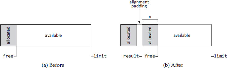
Figure 7.1: Sequential allocation: a call to sequentialAllocate(n) which advances the free pointer by the size of the allocation request, n, plus any padding necessary for proper alignment.

•  It is simple.

•  It is efficient, although Blackburn et al [2004a] have shown that the fundamental performance difference between sequential allocation and segregated-fits free-list allocation (see Section 7.4) for a Java system is on the order of 1% of total execution time.

•  It appears to result in better cache locality than does free-list allocation, especially for initial allocation of objects in moving collectors [Blackburn et al, 2004a].

•  It may be less suitable than free-list allocation for non-moving collectors, if uncollected objects break up larger chunks of space into smaller ones, resulting in many small sequential allocation chunks as opposed to one or a small number of large ones.

7.2    Free-list allocation

The alternative to sequential allocation is free-list allocation. In free-list allocation, a data structure records the location and size of free cells of memory. Strictly speaking, the data structure describes a set of free cells, and some organisations are in fact not list-like, but we will use the traditional term ‘free-list’ for them anyway. One can think of sequential allocation as a degenerate case of free-list allocation, but its special properties and simple implementation distinguish it in practice.

Algorithm 7.2: First-fit allocation

Algorithm 7.3: First-fit allocation: an alternative way to split a cell

We consider first the case of organising the set as a single list of free cells. The allocator considers each free cell in turn, and according to some policy, chooses one to allocate. This general approach is called sequential fits allocation, since the algorithm searches sequentially for a cell into which the request will fit. The classical versions of sequential fits are first-fit, next-fit and best-fit [Knuth, 1973, Section 2.5], which we now describe in turn.

First-fit allocation

When trying to satisfy an allocation request, a first-fit allocator will use the first cell it finds that can satisfy the request. If the cell is larger than required, the allocator may split the cell and return the remainder to the free-list. However, if the remainder is too small (allocation data structures and algorithms usually constrain the smallest allocatable cell size), then the allocator cannot split the cell. Further, the allocator may follow a policy of not splitting unless the remainder is larger than some absolute or percentage size threshold. Algorithm 7.2 gives code for first-fit. Notice that it assumes that each free cell has room to record its own size and the address of the next free cell. It maintains a single global variable head that refers to the first free cell in the list.

A variation that leads to simpler code in the splitting case is to return the portion at the end of the cell being split, illustrated in Algorithm 7.3. A possible disadvantage of this approach is the different alignment of objects, but this could cut either way. First-fit tends to exhibit the following characteristics [Wilson et al, 1995a, page 31]:

•  Small remainder cells accumulate near the front of the list, slowing down allocation.

•  In terms of space utilisation, it may behave rather similarly to best-fit since cells in the free-list end up roughly sorted from smallest to largest.

An interesting issue with first-fit is the order of cells in the list. When supporting explicit freeing, there are a number of options as to where in the list to enter a newly freed cell. For example, the allocator can insert the cell at the head, at the tail, or according to some order such as by address or size. When supporting garbage collection with a single free-list, it is usually more natural to build the list in address order, which is what a mark-sweep collector does.

Next-fit allocation

Next-fit is a variation of first-fit that starts the search for a cell of suitable size from the point in the list where the last search succeeded [Knuth, 1973]. This is the variable prev in the code sketched by Algorithm 7.4. When it reaches the end of the list it starts over from the beginning, and so is sometimes called circular first-fit allocation. The idea is to reduce the need to iterate repeatedly past the small cells at the head of the list. While next-fit is intuitively appealing, in practice it exhibits drawbacks.

•  Objects from different phases of mutator execution become mixed together. Because they become unreachable at different times, this can affect fragmentation (see Section 7.3).

•  Accesses through the roving pointer have poor locality because the pointer cycles through all the free cells.

•  The allocated objects may also exhibit poor locality, being spread out through memory and interspersed with objects allocated by previous mutator phases.

Best-fit allocation

Best-fit allocation finds the cell whose size most closely matches the request. The idea is to minimise waste, as well as to avoid splitting large cells unnecessarily. Algorithm 7.5 sketches the code. In practice best-fit seems to perform well for most programs, giving relatively low wasted space in spite of its bad worst-case performance [Robson, 1977]. Though such measurements were for explicit freeing, we would expect the space utilisation to remain high for garbage collected systems as well.

Algorithm 7.4: Next-fit allocation

 

Algorithm 7.5: Best-fit allocation

Algorithm 7.6: Searching in Cartesian trees

Speeding free-list allocation

Allocating from a single sequential list may not scale very well to large memories. Therefore researchers have devised a number of more sophisticated organisations of the set of free cells, to speed free-list allocation according to various policies. One obvious choice is to use a balanced binary tree of the free cells. These might be sorted by size (for best-fit) or by address (for first-fit or next-fit). When sorting by size, it saves time to enter only one cell of each size into the tree, and to chain the rest of the cells of that size from that tree node. Not only does the search complete faster, but the tree needs reorganisation less frequently since this happens only when adding a new size or removing the last cell of a given size.

To use balanced trees for first-fit or next-fit, one needs to use a Cartesian tree [Vuillemin, 1980]. This indexes by both address (primary key) and size (secondary key). It is totally ordered on addresses, but organised as a ‘heap’ for the sizes, which allows quick search for the first or next fit that will satisfy a given size request. This technique is also known as fast-fits allocation [Tadman, 1978; Standish, 1980; Stephenson, 1983]. A node in the Cartesian tree must record the address and size of the free cell, the pointers to the left and right child, and the maximum of the sizes of all cells in its subtree. It is easy to compute this maximum from the maximum values recorded in the node’s children and it own size. Hence the minimum possible size for a node is larger than for simple list-based schemes. While we omit code for inserting and removing nodes from the tree, to clarify the approach we give sample code for searching under the first-fit policy, in Algorithm 7.6. The code uses the single global variable root, which refers to the root of the binary tree. Each node n maintains a value max(n) that gives the maximum size of any nodes in that node’s subtree. Next-fit is only slightly more complicated than first-fit.

Balanced binary trees improve worst-case behaviour from linear to logarithmic in the number of free cells. Self-adjusting (splay) trees [Sleator and Tarjan, 1985] have similar (amortised time) benefits.

Another useful approach to address-ordered first-fit or next-fit allocation is bitmapped-fits allocation. A bitmap on the side has one bit for each granule of the allocatable heap. Rather than scanning the heap itself, we scan the bitmap. We can scan a byte at a time by using the byte value to index pre-calculated tables giving the size of the largest run of free granules within the eight-granule unit represented by the byte. The bitmap can also be augmented with run-length information that speeds calculating the size of larger free or allocated cells, in order to skip over them more quickly. Bitmaps have several virtues:

•  They are ‘on the side’ and thus less vulnerable to corruption. This is especially important for less safe languages such as C and C++, but also helpful in improving the reliability and debuggability of collectors for other, more safe, languages.

•  They do not require information to be recorded in the free and allocated cells, and thus minimise constraints on cell size. This effect can more than pay back the 3% storage overhead of one bit per 32-bit word. However, other considerations may require headers in objects, so this does not always hold.

•  They are compact, so scanning them causes few cache misses, thereby improving locality.

7.3    Fragmentation

At the beginning an allocation system generally has one, or a small number, of large cells of contiguous free memory. As a program runs, allocating and freeing cells, it typically produces a larger number of free cells, which can individually be small. This dispersal of free memory across a possibly large number of small free cells is called fragmentation. Fragmentation has at least two negative effects in an allocation system:

•  It can prevent allocation from succeeding. There can be enough free memory, in total, to satisfy a request, but not enough in any particular free cell. In non-garbage collected systems this generally forces a program to terminate. In a garbage collected system, it may trigger collection sooner than would otherwise be necessary.

•  Even if there is enough memory to satisfy a request, fragmentation may cause a program to use more address space, more resident pages and more cache lines than it would otherwise.

It is impractical to avoid fragmentation altogether. For one thing, the allocator usually cannot know what the future request sequence will be. For another, even given a known request sequence, optimal allocation — that is, using the smallest amount of space necessary for an entire sequence of allocate and free requests to succeed — is NP-hard [Robson, 1980]. However, some approaches tend to be better than others; while we cannot eliminate fragmentation, we have some hope of managing it. Generally speaking, we should expect a rough trade-off between allocation speed and fragmentation, while also expecting that fragmentation is quite difficult to predict in any given case.

For example, best-fit intuitively seems good with respect to fragmentation, but it can lead to a number of quite small fragments scattered through the heap. First-fit can also lead to a large number of small fragments, which tend to cluster near the beginning of the free-list. Next-fit will tend to distribute small fragments more evenly across the heap, but that is not necessarily better. The only total solution to fragmentation is compaction or copying collection.

7.4    Segregated-fits allocation

Much of the time consumed by a basic free-list allocator is spent searching for a free cell of appropriate size. Hence, using multiple free-lists whose members are segregated by size can speed allocation [Comfort, 1964]. In Chapter 9 we describe collectors that manage multiple spaces. While multiple spaces will almost always be managed using multiple allocators, when we speak of segregated-fits we mean multiple lists being used for allocating for the same (logical) space. The distinction is not always precise. For example, some collectors segregate large objects, or large objects that contain no outgoing references (such as images or other binary data). They do this partly for performance reasons, and perhaps also partly because such objects have different lifetime characteristics. The large objects may be in a different space, receiving different treatment during collection. Alternatively, each space may have a segregated set of large objects. The latter is more like segregated-fits, though smaller objects might be allocated sequentially rather than from a free-list. There are many ways to combine approaches.

The basic idea behind segregated-fits is that there is some number k of size values, s₀ < s₁ < ⋯ < s_k−1. The number k might vary, but is often fixed. There are k + 1 free-lists, f₀,…, f_k. The size b of a free cell on list f_i is constrained by s_i−1 < b ≤ s_i, where we set s₋₁ = 0 and s_k = +∞. Since the point is to avoid searching for a cell of suitable size, we restrict the condition further: the size of a free cell on list f_i must be exactly s_i. The one exception is f_k, which holds all cells larger than s_k−1, the largest size of the single-size lists. Thus, when requesting a cell of size b ≤ s_k−1, the allocator rounds the request size up to the smallest s_i such that b ≤ s_i. The sizes s_i are called size classes, and the size class for a cell size b is therefore that s_i such that s_i−1 < b ≤ s_i.

List f_k, for cells larger than s_k−1, is organised to use one of the basic single-list algorithms we previously presented. In this case a Cartesian tree or other data structure with good expected-time performance is probably a good choice. For one thing, larger objects are usually allocated less frequently. Even if that is not the case, just initialising them takes the application longer, so if the per-cell overheads are a bit higher for these larger cells than for allocating from the one-size lists, it will still not impact total execution time much as a percentage.

There are a variety of ways to speed the calculation of the size class s_i when given the desired object size b. For example, size classes s₀ through s_k−1 might be evenly spaced, that is, s_i = s₀ + c · i, for some suitable c > 0. Then the size class is s_k if b > s_k−1 and otherwise s_j where j = $\lfloor \left(b-s_0+c-1\right)/c\rfloor$ (using linear fit, where adding c − 1 does the appropriate rounding up). For example, an allocation scheme might have s₀ = 8, c = 8 and k = 16, giving size classes as multiples of eight from eight to 128 and using a general free-list algorithm for b > 128. The typical unit here is one byte, which makes sense for byte-addressed machines, as would a unit of one word for word-addressed machines. Still, even when bytes are the unit for describing size, a granule is more likely the size of a word, or even larger. Having c be a power of two speeds the division in the formula by allowing substitution of a shift for the generally slower division operation.

In addition to a very dense range of small size classes, a system might provide one or more ranges of somewhat larger sizes, less densely packed, as opposed to switching immediately to a general free-list mechanism. For example, the Boehm-Demers-Weiser collector has separate lists for each size from the minimum up to eight words, and then for even numbers of words up to 16, and for multiples of four words up to 32 [Boehm and Weiser, 1988]. Above that size it determines size classes somewhat dynamically, filling in an array that maps requested size (in bytes) to allocated size (in words). It then directly indexes an array of free-lists using the allocated size. Only those sizes used will be populated.

If the set of size classes is built in to a system (that is, fixed at system build time), then a compiler can in principle determine the appropriate free-list in advance for any allocation call whose size is known at compile time. This can substantially improve the common case cost for most allocations.

Algorithm 7.7: Segregated-fits allocation

To sum up concerning the time required to allocate a cell, schemes with single free-lists may search sequentially (first-fit, best-fit, and so on), which can take a long time to find a cell satisfying a given request. They may also use a balanced tree to attain worst-case or amortised logarithmic time. The particular advantage of segregated-fits is that for size classes other than s_k, allocation typically requires constant time, as shown in Algorithm 7.7; see also the lazy sweeping variant in Algorithm 2.5.

Fragmentation

In the simpler free-list allocators we discussed previously, there was only one kind of fragmentation: free cells that were too small to satisfy a request. This is known as external fragmentation, because it is unusable space outside any allocated cell. When we introduce size classes, if the sizes are at all spread out then there is also internal fragmentation, where space is wasted inside an individual cell because the requested size was rounded up. The need for specific alignment may introduce fragmentation in a similar way, although strictly speaking it is external fragmentation (between allocated cells). Segregated-fits introduces a trade-off between internal fragmentation and the number of size classes.

Populating size classes

It should now be reasonably clear how segregated-fits allocation works, except for the important consideration of how to populate each free-list. We discuss two approaches: dedicating whole blocks to particular sizes, also called big bag of pages (BiBoP), and splitting.

Big bag of pages block-based allocation. In this approach, we choose some block size B, a power of two. We provide an allocator for blocks, designed also to support requests for objects larger than one block by allocating multiple contiguous blocks. For a size class s < B, when we need more cells of size s we allocate a block and then immediately slice it into cells of size s, putting them on that free-list. Typically we also associate with the block the fact that it is dedicated to cells of size s. While that information might be stored in the block itself, along with other metadata such as mark bits for the cells in the block, Boehm and Weiser [1988] suggest that it is better to store this information in a separate area. Using a separate area results in fewer translation lookaside buffer misses or page faults when consulting or updating only the metadata, and it also avoids aligning every block’s metadata so that they compete for the same cache sets.

When we discussed lazy sweeping in Section 2.5, we described basic block-based allocation. Block-based allocation complicates the issue of fragmentation. Because we dedicate a whole block to cells of a given size, we will waste (on average) half a block, and we could waste up to the fraction (B – s)/B of the storage for a given size (if we have exactly one cell used in each block). However, we reduce the per-cell metadata. There is also some space waste if there is an unused portion of size less than s at the end of the block.¹ Whether we call these cases of unusable space internal or external fragmentation depends on our point of view: they are internal to a block, but external to cells.

In some systems the metadata associated with a cell includes not just the size s, but also the type of object allocated into the cell. While such segregation of types can result in greater fragmentation (since two types might be of the same size, but we must allocate them from separate blocks and maintain separate free-lists for them), for small objects the savings (by not having to record type information in each object) can be great. Examples include Lisp cons cells.

Beyond the combining of small cells’ metadata across an entire block, block-based allocation has the virtue of making the recombining of free cells particularly simple and efficient: it does not recombine unless all cells in a block are free, and then it returns the block to the block pool. Its common case for allocation, grabbing an available cell from a known list, is quite efficient, and if the list is empty, populating it is straightforward. Its primary disadvantage is its worst-case fragmentation.

Splitting. We have already seen cell splitting as a way to obtain cells of a given size s: the various simple free-list schemes will split a larger cell if that is the only way to satisfy a request. If we use a fairly dense collection of size classes, then when we split a cell, we will be likely to have a suitable free-list to receive the portion not allocated. There are some particular organisations of less dense size classes that also have that property. One such scheme is the buddy system, which uses sizes that are powers of two [Knowlton, 1965; Peterson and Norman, 1977]. It is clear that we can split a cell of size 2ⁱ⁺¹ into two cells of size 2ⁱ. We can also recombine (or coalesce) two adjacent cells of size 2ⁱ into one cell of size 2ⁱ⁺¹. A buddy system will only recombine that way if the cells were split from the same cell of size 2ⁱ⁺¹ originally. Hence cells of size 2ⁱ come in pairs, that is, are buddies. Given the high internal fragmentation of this approach (its average is 25% for arbitrarily chosen allocation requests), it is now largely of historical as opposed to practical interest.

A variation of the 2ⁱ buddy system is the Fibonacci buddy system [Hirschberg, 1973; Burton, 1976; Peterson and Norman, 1977], in which the size classes form a Fibonacci sequence: s_i+2 = s_i+1 + s_i, with a suitable s₀ and s₁ to start. Because the ratio of adjacent sizes is smaller than in the power-of-two buddy system, the average internal fragmentation will be lower (as a percentage of allocated memory). However, locating adjacent cells for re-combining free cells after collection is slightly more complicated, since a buddy can have the next size larger or smaller depending on which member of a buddy pair is under consideration.

Other variations on the buddy system have been described by Wise [1978], Page and Hagins [1986] and Wilson et al [1995b].

7.5    Combining segregated-fits with first-, best- and next-fit

We can use segregated-fits as an accelerating front end to the schemes that use a single free-list. In this case, we place a cell that falls into a given size class onto the list for that class. If a request finds that the free-list for its size class is empty, we can implement best-fit by searching the larger size classes in order of increasing size looking for a non-empty free-list. Having a segregated-fits front end modifies first- and next-fit, leading to a design choice of what to do when the free-list for the desired size class is empty. But in any case, if we end up searching list f_k, the list of all cells of size greater than s_k−1, then we apply the single-list scheme (first-fit, best-fit or next-fit).

Another way of seeing this is that we really have a segregated-fits scheme, and are simply deciding how we are going to manage f_k. To summarise, we can manage it in these ways:

•  As a single free-list, using first-fit, best-fit, next-fit or one of the variations on them previously discussed, including Cartesian trees or other data structures that reduce search time.

•  Using block-based allocation.

•  Using a buddy system.

7.6    Additional considerations

Actual allocators often must take into account some additional considerations. We now discuss these: alignment, size constraints, boundary tags, heap parsability, locality, wilderness preservation and crossing maps.

Alignment

Depending on constraints of the underlying machine and its instruction set, or for better packing and improved memory hierarchy performance (cache, translation lookaside buffer or paging), an allocated object may require special alignment. For example, consider a Java array of double. On some machines, the double-word floating point values must be aligned on double-word boundaries, that is, their addresses must be 0 modulo 8 (with the three low bits of the address equal to zero). One way to address the overall problem is to make double-words the granule of allocation. In that case, all allocated and free cells are a multiple of eight bytes in size, and are aligned on an eight-byte boundary. This is simple, but perhaps slightly wasteful. Further, when allocating an array of double, there is still some special work that might be required. Suppose that the Java heap design requires two header words for scalar (non-array) objects, one to refer to the object’s class information (for virtual method dispatch, type determination and so on) and one for the object’s hash code and Java synchronisation (locking). This is a typical design. Array objects require a third word, giving the number of elements in the array. If we store these three header words at the start of the allocated space and follow them immediately by the array elements, the elements will be aligned on an odd word boundary, not an even one as required. If we use double-words as the granule, then we simply use four words (two double-words) for the three-word header and waste a word.

But suppose our granule is one word, and we wish to avoid wasting a word whenever we can. In that case, if a free cell we are considering is aligned on an odd word boundary (that is, its address is 4 modulo 8), we can simply use the cell as is, putting the three header words first, immediately followed by the array element, which will be doubleword aligned as required. If the cell starts on an even word boundary, we have to skip a word to get the proper alignment. Notice that this complicates our determination of whether a request will fit in a given cell: it may or may not fit, depending on the required and actual alignment — see Algorithm 7.8.

Algorithm 7.8: Incorporating alignment requirements

Size constraints

Some collection schemes require a minimum amount of space in each object (cell) for managing the collection process. For example, basic compacting collection needs room for the new address in each object. Some collectors may need two words, such as a lock/status word plus a forwarding pointer. This implies that even if the language needs only one word, the allocator will still need to allocate two words. In fact, if a program allocates some objects that contain no data and serve only as distinct unique identifiers, for some languages they could in principle consume no storage at all! In practice this does not work since the address of the object forms its unique identity (or else you must calculate a unique value and store it in the object), so the object must consume at least one byte.

Boundary tags

In order to support recombination when freeing objects, many allocate-free systems associate an additional header or boundary tag with each cell, outside the storage available to the program [Knuth, 1973]. The boundary tag indicates the size of the cell and whether it is allocated or free. It may also indicate the size of the previous cell, making it easier to find its flag indicating whether it is free, and its free-list chaining pointers if it is free. Thus, a boundary tag may be two words long, though with additional effort and possibly more overhead in the allocation and freeing routines, it may be possible to pack it into one word.

Using bitmaps on the side to indicate which granules are allocated and free avoids the need for boundary tags, and may be more robust as we previously observed. Which approach uses less storage depends on the average object size and the allocation granularity.

We further observe that because garbage collection frees objects all at once, a given algorithm may not need boundary tags, or may need less information in them. Further, in managed languages we will generally know the size of a cell by examining its type and so do not need to record that information separately.

Heap parsability

The sweeping phase of a mark-sweep collector must be able to advance from cell to cell in the heap. This capability is what we call heap parsability. Other kinds of collectors may not require parsability, but it can be a great help in debugging collectors so it is good to support parsability if possible and the cost is not too high.

Generally we need parsability only in one direction, most commonly in order of increasing address. A typical language will use one or two words to record an object’s type and other necessary information. We call this the object’s header. For example, many Java implementations use one word to record what amounts to a type (a pointer to type information, including a vector of addresses of methods of the object’s class) and one word for a hash code, synchronisation information, garbage collection mark bit and so on. In order to make indexing into arrays efficient on most machines, it helps if the object reference refers to the first element of the array, with successive elements at successively higher addresses. Since the language run-time and the collector need to find the type of an object in a uniform way given a reference to the object, we place the header immediately before the object data. Thus, the object reference points not to the first allocated byte, but into the middle of the allocated cell, after the header. Having the header come before the object contents therefore facilitates upward parsing of the heap.

Figure 7.2: A Java object header design for heap parsability. Grey indicates the words forming the referent object. Neighbouring objects are shown with dashed lines.

Again using a Java system as an example, array instances need to record the length of the individual array. For easy parsability, it helps if the length field comes after the two-word header used for every object. Therefore the first array element falls at the third word of the allocated cell, the length is at word −1 and the rest of the header is at words −2 and −3. A scalar (non-array) object needs to place its header at words −2 and −3 as well. This would appear to leave word −1 as a ‘hole’, but in fact there is no problem placing the first (scalar) field of the object there (assuming that the machine can index by a small negative constant just as well as by a small positive one, and most can). Further, if the object has no additional fields, there is still no problem: the header of the next object can legally appear at the address to which the object reference points! We illustrate all this in Figure 7.2.

A particular issue arises if an implementation desires to over-write one object with another (necessarily smaller) one, as a number of functional language implementations do in replacing a closure with its evaluated value. If the implementation takes no further action, a scan that parses the heap may land in the middle of ‘unformatted’ bits and get quite confused. Non-Stop Haskell solves this problem by inserting filler objects [Cheadle et al, 2004]. In the usual case they need only to insert a reference to metadata indicating a pointer-free object of the appropriate size; they pre-construct metadata for sizes one through eight words. Larger fillers are quite rare, but would require creating metadata dynamically.²

One final consideration arises from alignment requirements. If an individual object needs to be shifted one or more words from the beginning of its cell for proper alignment, we need to record something in the gap so that in heap parsing we will know to skip. If ordinary object headers cannot begin with an all-zero word, and if we zero all free space in advance, then when parsing we can simply skip words whose value is zero. A simple alternative is to devise a distinct range of values to write at the start of gap, identifying it as a gap and giving its length. For example, Sun have long used what they call a ‘self-parsing’ heap. When they free an object (in a non-moving space), they overwrite its memory with a filler object, which includes a field giving its size (think of it as an array of words). This is particularly useful for skipping ahead to the next real object when sweeping the heap.

A bitmap on the side, indicating where each object starts, makes heap parsing easy and simplifies the design constraints on object header formats. However, such bits consume additional space and require additional time to set during allocation. Allocation bitmaps are useful in many collectors, especially parallel and concurrent ones.

While we mentioned a design for Java, similar considerations apply to other languages. Furthermore, block-based allocation offers simple parsing for the small cells, and it is also easy to handle the large blocks. For improved cache performance, the location of a large object inside a sequence of one or more blocks is something we might randomise, that is, we randomise how much of the wasted space comes before, and how much after, the application object. It is easy to record at the start of the block where the object is, in order to support parsability.

Locality

Locality issues come up several ways in allocation. There is locality of the allocation process itself, and of freeing. Other things being equal, an address-ordered free-list may improve locality of allocator memory accesses. Sequential allocation also leads naturally to sequential accesses with good locality. In fact, software prefetching a bit ahead of the allocator can help [Appel, 1994], though for certain hardware that is unnecessary [Diwan et al, 1994]. But there is an entirely different notion of locality that is also useful to consider: objects that may become unreachable at about the same time. If some objects become unreachable at the same time, and they are allocated adjacent to one another, then after collection their space will coalesce into a single free chunk, thus minimising fragmentation. Empirically, objects allocated at about the same time often become unreachable at about the same time. This makes non-moving systems less problematic than might be presumed [Hayes, 1991; Dimpsey et al, 2000; Blackburn and McKinley, 2008]. It also suggests applying a heuristic of trying to allocate next to, or at least near, the most recently allocated object. Specifically, if the previous allocation request was satisfied by splitting a larger chunk, then it can help reduce fragmentation to prefer splitting the same chunk for requests in the near future, if the future request cannot be satisfied directly from a free-list for objects of the appropriate size.

Wilderness preservation

A typical heap organisation consists of a large contiguous part of the machine’s address space, often bounded at the low end by the program’s static code and data areas. The other end is often not occupied, but rather is open for expansion. This boundary in Unix systems is called the ‘break’ and the sbrk call can grow (or shrink) the available space by adjusting the boundary. Space beyond the boundary may not even be in the virtual memory map. The last free chunk in the heap is thus expandable. Since it begins what could be called ‘unoccupied territory,’ it is called the wilderness, and Korn and Vo [1985] found that wilderness preservation — allocating from the wilderness only as a last resort — helped reduce fragmentation. It also has the salutary effect of tending to defer the need to grow the heap, and thus conserves overall system resources.

Crossing maps

Some collection schemes, or their write barriers, require the allocator to fill in a crossing map. This map indicates, for each aligned segment of the heap of size 2^k for some suitable k, the address (or offset within the 2^k segment) of the last object that begins in that segment. Combined with heap parsability, this allows a barrier or collector to determine fairly quickly, from an address within an object, the start of the object, and thus to access the object’s headers, and so on. We discuss crossing maps in more detail in Section 11.8.

7.7    Allocation in concurrent systems

If multiple threads attempt to allocate simultaneously, then since most steps in allocation need to be atomic to preserve the integrity of the allocation data structures, they will need to use atomic operations or locks. Allocation can thus become a serial bottleneck. The basic solution is to give each thread its own allocation area. If a thread runs out, it can obtain another chunk of free space in which to allocate from a global pool. Only interactions with the global pool need to be atomic. Individual threads may vary in their allocation rates, so to improve both time and space performance it can help to employ an adaptive algorithm to adjust the size of the free space chunks handed out to each thread — a slowly allocating thread might receive a small chunk while a rapidly allocating one gets a large chunk. Dimpsey et al [2000] noted substantial performance improvement in a multiprocessor Java system using a suitably organised local allocation buffer (LAB) for each thread.³ They further note that since the local allocation buffers absorb almost all allocation of small objects, it was beneficial to retune the global free-list-based allocator since its typical request was for a new local allocation buffer chunk.

Garthwaite et al [2005] discussed adaptive sizing of local allocation buffers, and found benefit from associating them with processors rather than threads. They describe the original mechanism for sizing per-thread local allocation buffers as follows. Initially a thread requests a 24-word (96 byte) local allocation buffer. Each time it requests another local allocation buffer, it multiplies the size by 1.5. However, when the collector runs, it decays each thread’s local allocation buffer size by dividing by two. The scheme also involves adjustment to the young generation’s size according to the number of different threads allocating. The per-processor local allocation buffer scheme relies on multiprocessor restartable critical sections, which Garthwaite et al introduced. This mechanism allows a thread to determine whether it has been preempted and rescheduled, which implies that it may be running on a different processor. By having such preemption modify a register used in addressing the per-processor data, they can cause stores after preemption to produce a trap, and the trap handler can restart the interrupted allocation. Even though per-processor local allocation buffers involve more instructions, their latency was the same, and they required less sophisticated sizing mechanisms to work well. They also found that for small numbers of threads, per-thread local allocation buffers were better (consider especially the case where there are fewer threads than processors), and per-processor local allocation buffers were better when there are many allocating threads. Therefore, they designed their system to support switching between the two approaches dynamically.

A typical local allocation buffer is used for sequential allocation. Another design is for each thread (or processor) to maintain its own set of segregated free-lists, in conjunction with incremental sweeping. When a thread sweeps a block incrementally during allocation, it puts the free cells into its own free-lists. This design has certain problems that arise when it is used for explicit storage management, as addressed by Berger et al [2000]. For example, if the application uses a producer-consumer model, then the producer allocates message buffers and the consumer frees them, leading to a net transfer of buffers from one to the other. In the garbage collected world, the collection process may return buffers to a global pool. However, incremental sweeping that places free cells on the sweeper’s free-lists naturally returns free buffers to threads that allocate them most frequently.

7.8    Issues to consider

There are some particular issues to consider when designing an allocator for a garbage collected system: Allocation cannot be considered independently of the collection algorithm. In particular, non-moving collectors such as mark-sweep more or less demand a free-list approach as opposed to sequential allocation — but see Section 10.3 for contrary views on this, and some local allocation buffer approaches also use sequential allocation in conjunction with mark-sweep collection. Conversely, sequential allocation makes the most sense for copying and compacting collectors, because it is fast and simple. It is not necessarily much faster than segregated-fits free-list allocation, but its simplicity may offer better overall reliability.

If a collector uses mark-sweep but offers occasional or emergency compaction to eliminate fragmentation, then it needs to provide for updating the allocation data structures to reflect the state of the world after compaction.

Bitmaps on the side for recording free/allocated granules and where cells or objects start add robustness and simplify object header design. They can also speed collector operations and improve the collector’s memory hierarchy performance. Their space cost is modest, but they do add some time cost during allocation, even in the common case.

Block-based allocation can reduce per-object overheads, both for the language implementation (for example, if a block is dedicated to objects of a single type) and for collector metadata. This may be offset by the space consumed by unallocated cells and the unusable space within some blocks. Block-based allocation may also fit well with organisations that support multiple spaces with different allocation and collection techniques.

Segregated-fits is generally faster than single free-list schemes. This is of greater importance in a garbage collected context since programs coded assuming garbage collection tend to do more allocation than ones coded using explicit freeing.

Because a collector frees objects in batches, the techniques designed for recombining free cells for explicit freeing systems are less relevant. The sweep phase of mark-sweep can rebuild a free-list efficiently from scratch. In the case of compacting collectors, in the end there is usually just one large free chunk appropriate for sequential allocation. Copying similarly frees whole semispaces without needing to free each individual cell.

¹Boehm and Weiser [1988] place this portion at the start of the block rather than its end, presumably to reduce competition for cache lines near the beginning of blocks. This helps more for small cache lines, since it is effective only for (some) cell sizes large than a cache line.

²They do not offer details, but it seems reasonable to us to place the metadata in the filler in that case, thus avoiding any run-time allocation to restore heap parsability.

³Some authors use the term ‘thread-local heap’. We use local allocation buffer when the point is separate allocation, and reserve use of ‘thread-local heap’ for the case where the local areas are collected separately. Thus, while a ‘thread-local heap’ is almost certainly a local allocation buffer, the reverse need not be true.