
![]()
SQL Execution
You likely learned the mechanics of writing basic SQL in a relatively short period of time. Throughout the course of a few weeks or few months, you became comfortable with the general statement structure and syntax, how to filter, how to join tables, and how to group and order data. But, how far beyond that initial level of proficiency have you traveled? Writing complex SQL that executes efficiently is a skill that requires you to move beyond the basics. Just because your SQL gets the job done doesn’t mean it does the job well.
In this chapter, I’m going to raise the hood and look at how SQL executes from the inside out. I’ll discuss basic Oracle architecture and introduce the cost-based query optimizer. You’ll learn how and why the way you formulate your SQL statements affects the optimizer’s ability to produce the most efficient execution plan possible. You may already know what to do, but understanding how SQL execution works will help you help Oracle accomplish the results you need in less time and with fewer resources.
Oracle Architecture Basics
The SQL language is seemingly easy enough that you can learn to write simple SQL statements in fairly short order. But, just because you can write SQL statements that are functionally correct (in other words, produce the proper result set) doesn’t mean you’ve accomplished the task in the most effective and efficient way.
Moving beyond basic skills requires deeper understanding. For instance, when I learned to drive, my father taught me the basics. We walked around the car and discussed the parts of the car that he thought were important to be aware of as the driver of the vehicle. We talked about the type of gas I should put in the car, the proper air pressure for the tires, and the importance of getting regular oil changes. Being aware of these things would help make sure the vehicle was in good condition when I wanted to drive it.
He then taught me the mechanics of driving. I learned how to start the engine, shift gears, increase and decrease my speed, use the brake, use turn signals, and so on. But, what he didn’t teach me was specifically how the engine worked, how to change the oil myself, or anything else other than what I needed to do to allow me to drive the vehicle safely from place to place. If I needed my car to do anything aside from what I learned, I had to take it to a professional mechanic, which isn’t a bad thing. Not everyone needs to have the skills and knowledge of a professional mechanic just to drive a car. However, the analogy applies to anyone who writes SQL. You can learn the basics and be able to get your applications from place to place; but, without extending your knowledge, I don’t believe you’ll ever be more than an everyday driver. To get the most out of SQL, you need to understand how it does what it does, which means you need to understand the basics of the underlying architecture on which the SQL you write will execute.
Figure 2-1 depicts how most people view the database when they first learn to write SQL. It is simply a black box to which they direct SQL requests and from which they get data back. The “machinery” inside the database is a mystery.
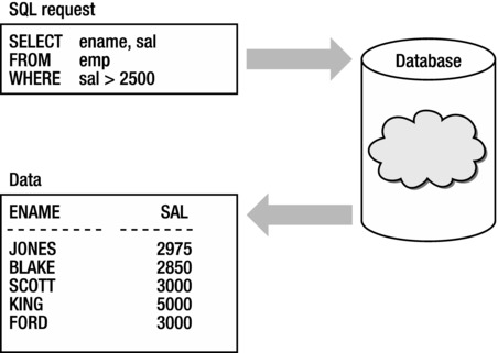
Figure 2-1. Using SQL and the database
The term Oracle database is typically used to refer to the files, stored on disk, where data reside along with the memory structures used to manage those files. In reality, the term database belongs to the data files; the term instance belongs to the memory structures and the processes. An instance consists of the system global area (SGA) and a set of background processes. Each user connection to the database is managed via a server process. Each client connection is associated with server processes that are each allocated their own private memory area called the program, or process, global area (PGA).
The Oracle Concepts Guide goes into detail about each of the memory structures and processes. I think it’s a great idea for everyone who will use Oracle to read the Oracle Concepts Guide. For our purposes, however, I limit my discussion to a few key areas to help you understand how SQL operates. Specifically, I review two areas of the SGA: the shared pool (specifically, the library cache within the shared pool) and the database buffer cache. Later in the book, I discuss some particulars about the PGA, but for now, I’m keeping our review limited to the SGA . Note that these discussions will present a fairly broad picture. As I said, I don’t want to overwhelm you, but I do think this is critical information on which to get a grasp before you go any further.
SGA: The Shared Pool
The shared pool is one of the most critical memory components, particularly when it comes to how SQL executes. The way you write SQL affects more than the individual SQL statement itself. The combination of all SQL that executes against the database has a tremendous effect on overall performance and scalability resulting from how it affects the shared pool.
The shared pool is where Oracle caches program data. Every SQL statement executed has its parsed form stored in the shared pool. The area within the shared pool where statements are stored is called the library cache. Even before any statement is parsed, Oracle checks the library cache to determine whether that same statement already exists there. If it does, then Oracle retrieves and uses the cached information instead of going through all the work to parse the same statement again. The same thing goes for any PL/SQL (PL/SQL is Oracle’s Procedural Language extension to SQL) code you run. The really nifty part is that, no matter how many users may want to execute the same SQL statement, Oracle typically only parses that statement once and then shares it among all users who want to use it. Now maybe you can understand why the shared pool gets its name.
SQL statements you write aren’t the only things stored in the shared pool. The system parameters Oracle uses are stored in the shared pool as well. In an area called the dictionary cache, Oracle also stores information about all the database objects. In general, Oracle stores pretty much everything you can think of in the shared pool. As you can imagine, this makes the shared pool a very busy and important memory component.
Because the memory area allocated to the shared pool is finite, statements that get loaded originally may not stay there for very long as new statements are executed. A least recently used (LRU) algorithm regulates how objects in the shared pool are managed. To borrow an accounting term, it’s similar to a FIFO (first in; first out) system. The basic idea is that statements that are used most frequently and most currently are retained. Unlike a straight FIFO method, however, how frequently the same statements are used affects how long they remain in the shared pool. If you execute a SELECT statement at 8 AM and then execute the same statement again at 4 PM, the parsed version that was stored in the shared pool at 8 AM may not still be there. Depending on the overall size of the shared pool and how much activity it has seen between 8 AM and 4 PM—Oracle needs space to store the latest information throughout the day—it simply reuses older areas and overlays newer information into them. But, if you execute a statement every few seconds throughout the day, the frequent reuse causes Oracle to retain that information over something else that may have been originally stored later than your statement but hasn’t been executed frequently, or at all, since it was loaded.
One of the things you need to keep in mind as you write SQL is that, to use the shared pool most efficiently, statements need to be shareable. If every statement you write is unique, you basically defeat the purpose of the shared pool. The less shareable it is, the more effect you’ll see on overall response times. I show you exactly how expensive parsing can be in the next section.
The Library Cache
The first thing that must happen to every SQL statement you execute is that it must be parsed and loaded into the library cache. The library cache, as mentioned earlier, is the area within the shared pool that holds previously parsed statements. Parsing involves verifying the statement syntax, validating objects being referred to, and confirming user privileges on the objects. If these checks are passed, the next step is for Oracle to determine whether that same statement has been executed previously. If it has, then Oracle grabs the stored information from the previous parse and reuses it. This type of parse is called a soft parse. If the statement hasn’t been executed previously, then Oracle does all the work to develop the execution plan for the current statement and then stores it in the cache for later reuse. This type of parse is called a hard parse.
Hard parses require Oracle to do a lot more work than soft parses. Every time a hard parse occurs, Oracle must gather all the information it needs before it can actually execute the statement. To get the information it needs, Oracle executes a bunch of queries against the data dictionary. The easiest way to see what Oracle does during a hard parse is to turn on extended SQL tracing, execute a statement, and then review the trace data. Extended SQL tracing captures every action that occurs, so not only do you see the statement you execute, but also you see every statement that Oracle must execute as well. Because I haven’t covered the details of how tracing works and how to read a trace file, I’m not going to show the detailed trace data. Instead, Table 2-1 provides the list of system tables that were queried during a hard parse of select * from employees where department_id = 60.
Table 2-1. System Objects Queried during Hard Parse
| Tables | No. of Queries | Purpose |
|---|---|---|
| aud_object_opt$ | 1 | Object audit data |
| ccol$ | 1 | Constraint column-specific data |
| cdef$ | 4 | Constraint-specific definition data |
| col$ | 1 | Table column-specific data |
| hist_head$ | 1 | Histogram header data |
| histgrm$ | 1 | Histogram specifications |
| icol$ | 1 | Index columns |
| ind$ | 1 | Indexes |
| ind_stats$ | 1 | Index statistics |
| obj$ | 3 | Objects |
| objauth$ | 2 | Table authorizations |
| opt_directive_own$ | 1 | SQL plan directives |
| seg$ | 1 | Mapping of all database segments |
| tab$ | 2 | Tables |
| tab_stats$ | 1 | Table statistics |
| user$ | 2 | User definitions |
In total, there were 19 queries against system objects executed during the hard parse. This number, from version 12c, is less than the version 11g total of 59 for the same query. The soft parse of the same statement did not execute any queries against the system objects because all that work was done during the initial hard parse. The elapsed time for the hard parse was 0.030641 second whereas the elapsed time for the soft parse was 0.000025 second. As you can see, soft parsing is a much more desirable alternative to hard parsing. Don’t ever fool yourself into thinking parsing doesn’t matter. It does!
For Oracle to determine whether a statement has been executed previously, it checks the library cache for the identical statement. You can see which statements are currently stored in the library cache by querying the v$sql view. This view lists statistics on the shared SQL area and contains one row for each “child” of the original SQL text entered. Listing 2-1 shows three different executions of a query against the employees table followed by a query against v$sql showing information about the three queries that have been stored in the library cache.
Listing 2-1.Queries against Employees and v$sql Contents
SQL> select * from employees where department_id = 60;

    EMPLOYEE_ID FIRST_NAME           LAST_NAME                 EMAIL
--------------- -------------------- ------------------------- -----------
            103 Alexander            Hunold                    AHUNOLD
            104 Bruce                Ernst                     BERNST
            105 David                Austin                    DAUSTIN
            106 Valli                Pataballa                 VPATABAL
            107 Diana                Lorentz                   DLORENTZ

SQL> SELECT * FROM EMPLOYEES WHERE DEPARTMENT_ID = 60;

    EMPLOYEE_ID FIRST_NAME           LAST_NAME                 EMAIL
--------------- -------------------- ------------------------- -----------
            103 Alexander            Hunold                    AHUNOLD
            104 Bruce                Ernst                     BERNST
            105 David                Austin                    DAUSTIN
            106 Valli                Pataballa                 VPATABAL
            107 Diana                Lorentz                   DLORENTZ

SQL> select /* a_comment */ * from employees where department_id = 60;

    EMPLOYEE_ID FIRST_NAME           LAST_NAME                 EMAIL
--------------- -------------------- ------------------------- -----------
            103 Alexander            Hunold                    AHUNOLD
            104 Bruce                Ernst                     BERNST
            105 David                Austin                    DAUSTIN
            106 Valli                Pataballa                 VPATABAL
            107 Diana                Lorentz                   DLORENTZ

SQL> select sql_text, sql_id, child_number, hash_value, executions
 2   from v$sql where upper(sql_text) like '%EMPLOYEES%';

SQL_TEXT                    SQL_ID        CHILD_NUMBER HASH_VALUE EXECUTIONS
--------------------------- ------------- ------------ ---------- ----------
select * from employees     0svc967bxf4yu            0 3621196762          1
 where department_id = 60
SELECT * FROM EMPLOYEES     cq7t1xq95bpm8            0 2455098984          1
 WHERE DEPARTMENT_ID = 60
select /* a_comment */ *    2dkt13j0cyjzq            0 1087326198          1
  from employees
 where department_id = 60
Although all three statements return the exact same result, Oracle considers them to be different. This is because, when a statement is executed, Oracle first converts the string to a hash value. That hash value is used as the key for that statement when it is stored in the library cache. As other statements are executed, their hash values are compared with the existing hash values to find a match.
So, why would these three statements produce different hash values, even though they return the same result? Because the statements are not identical. Lowercase text is different from uppercase text. Adding a comment into the statement makes it different from the statements that don’t have a comment. Any differences cause a different hash value to be created for the statement, and cause Oracle to hard parse the statement.
The execution of statements that differ only by their literals can cause significant parsing overhead, which is why it is important to use bind variables instead of literals in your SQL statements. When you use a bind variable, Oracle is able to share the statement even as you change the values of the bind variables, as shown in Listing 2-2.
Listing 2-2. The Effect of Using Bind Variables on Parsing
SQL> variable v_dept number
SQL> exec :v_dept := 10
SQL> select * from employees where department_id = :v_dept;

    EMPLOYEE_ID FIRST_NAME           LAST_NAME                 EMAIL
--------------- -------------------- ------------------------- -----------
            200 Jennifer             Whalen                    JWHALEN

1 row selected.

SQL> exec :v_dept := 20

PL/SQL procedure successfully completed.

SQL> select * from employees where department_id = :v_dept;

    EMPLOYEE_ID FIRST_NAME           LAST_NAME                 EMAIL
--------------- -------------------- ------------------------- -----------
            201 Michael              Hartstein                 MHARTSTE
            202 Pat                  Fay                       PFAY

2 rows selected.

SQL> exec :v_dept := 30

PL/SQL procedure successfully completed.

SQL> select * from employees where department_id = :v_dept;

    EMPLOYEE_ID FIRST_NAME           LAST_NAME                 EMAIL
--------------- -------------------- ------------------------- -----------
            114 Den                  Raphaely                  DRAPHEAL
            115 Alexander            Khoo                      AKHOO
            116 Shelli               Baida                     SBAIDA
            117 Sigal                Tobias                    STOBIAS
            118 Guy                  Himuro                    GHIMURO
            119 Karen                Colmenares                KCOLMENA

6 rows selected.

SQL> select sql_text, sql_id, child_number, executions
 2   from v$sql where sql_text like '%v_dept';

SQL_TEXT                        SQL_ID        CHILD_NUMBER EXECUTIONS
------------------------------- ------------- ------------ ----------
select * from employees         72k66s55jqk1j            0          3
 where department_id = :v_dept

1 row selected.
Notice how there is only one statement with three executions stored in the library cache. If I had executed the queries using the literal values (10, 20, 30), there would have been three different statements. Always keep this in mind and try to write SQL that takes advantage of bind variables and uses exactly the same SQL. The less hard parsing that is required means your applications perform better and are more scalable.
There are two final mechanisms that are important to understand. The first is something called a latch. A latch is a type of lock that Oracle must acquire to read information stored in the library cache as well as other memory structures. Latches protect the library cache from becoming corrupted by concurrent modifications by two sessions, or by one session trying to read information that is being modified by another one. Before reading any information from the library cache, Oracle acquires a latch that then causes all other sessions to wait until that latch is released before they can acquire the latch and do the work they need to complete.
This is a good place to mention the second mechanism: the mutex. A mutex (mutual exclusion lock) is similar to a latch in that it is a serialization device used to prevent multiple threads from accessing shared structures simultaneously. The biggest advantage of mutexes over latches is that mutexes require less memory and are faster to acquire and release. Also, mutexes are used to avoid the need to get the library cache latch for a previously opened cursor (in the session cursor cache) by modifying the cursor’s mutex reference count directly. A mutex is a better performing and more scalable mechanism than a latch. Note that library cache latching is still needed for parsing, however.
Latches, unlike typical locks, are not queued. In other words, if Oracle attempts to acquire a latch on the library cache to determine whether the statement you are executing already exists, it checks whether the latch is available. If the latch is available, it acquires the latch, does the work it needs to do, then releases the latch. However, if the latch is already in use, Oracle does something called spinning. Think of spinning as repetitive—like a kid in the backseat of a car asking, “Are we there yet?” over and over and over. Oracle basically iterates in a loop, and continues to determine whether the latch is available. During this time, Oracle is actively using the central processing unit (CPU) to do these checks, but your query is actually “on hold” and not really doing anything until the latch is acquired.
If the latch is not acquired after spinning for a while (Oracle spins up to the number of times indicated by the _spin_count hidden parameter, which is set to 2000 by default), then the request is halted temporarily and your session has to get in line behind other sessions that need to use the CPU. It must wait its turn to use the CPU again to determine whether the latch is available. This iterative process continues until the latch can be acquired. You don’t just get in line and wait on the latch to become available; it’s entirely possible that another session acquires the latch while your session is waiting in line to get back on the CPU to check the latch again. As you can imagine, this can be quite time-consuming if many sessions all need to acquire the latch concurrently.
The main thing to remember is that latches and mutexes are serialization devices. The more frequently Oracle needs to acquire one, the more likely it is that contention will occur, and the longer you’ll have to wait. The effects on performance and scalability can be dramatic. So, writing your code so that it requires fewer mutexes and latches (in other words, less hard parsing) is critical.
The buffer cache is one of the largest components of the SGA. It stores database blocks after they have been read from disk or before they are written to disk. A block is the smallest unit with which Oracle works. Blocks contain rows of table data or index entries, and some blocks contain temporary data for sorts. The key thing to remember is that Oracle must read blocks to get to the rows of data needed to satisfy a SQL statement. Blocks are typically either 4KB, 8KB, or 16KB, although the only restricting factor to the size of a block depends on your operating system.
Each block has a certain structure. Within the block there are a few areas of block overhead that contain information about the block itself that Oracle uses to manage the block. There is information that indicates the type of block it is (table, index, and so forth), a bit of information about transactions against the block, the address where the block resides physically on the disk, information about the tables that store data in the block, and information about the row data contained in the block. The rest of the block contains either the actual data or free space where new data can be stored. There’s more detail about how the buffer cache can be divided into multiple pools and how it has varying block sizes, but I’ll keep this discussion simple and just consider one big default buffer pool with a single block size.
At any given time, the blocks in the buffer cache will either be dirty, which means they have been modified and need to be written into a physical location on the disk, or not dirty. During the earlier discussion of the shared pool, I mentioned the LRU algorithm used by Oracle to manage the information there. The buffer cache also uses an LRU list to help Oracle know which blocks are used most recently to determine how to make room for new blocks as needed. Besides the LRU list, Oracle maintains a touch count for each block in the buffer cache. This count indicates how frequently a block is used; blocks with higher touch counts remain in the cache longer than those with lower touch counts.
Also similar to the shared pool, latches must be acquired to verify whether blocks are in the buffer cache, and to update the LRU information and touch counts. One of the ways you can help Oracle use less latches is to write your SQL in such a way that it accesses the fewest blocks possible when trying to retrieve the rows needed to satisfy your query. I discuss how you can do this throughout the rest of the book, but for now, keep in mind that, if all you think about when writing a SQL statement is getting the functionally correct answer, you may write your SQL in such a way that it accesses blocks inefficiently and therefore uses more latches than needed. The more latches required, the more chance for contention, and the more likely your application will be less responsive and less scalable than others that are better written.
Executing a query with blocks that are not in the buffer cache requires Oracle to make a call to the operating system to retrieve those blocks and then place them in the buffer cache before returning the result set to you. In general, any block that contains rows needed to satisfy a query must be present in the buffer cache. When Oracle determines that a block already exists in the buffer cache, such access is referred to as a logical read. If the block must be retrieved from disk, it is referred to as a physical read. As you can imagine, because the block is already in memory, response times to complete a logical read are faster than physical reads. Listing 2-3 shows the differences between executing the same statement multiple times under three scenarios. First, the statement is executed after clearing both the shared pool and the buffer cache. This means that the statement will be hard parsed, and the blocks that contain the data to satisfy the query (and all the queries from the system objects to handle the hard parse) have to be read physically from disk. The second example shows what happens if only the buffer cache is cleared. The third example shows what happens if both the shared pool and buffer cache are populated.
Listing 2-3. Hard Parsing and Physical Reads Versus Soft Parsing and Logical Reads
SQL> alter system flush buffer_cache;

System altered.

SQL> alter system flush shared_pool;

System altered.

SQL> set autotrace traceonly statistics
SQL>
SQL> select * from employees where department_id = 60;

5 rows selected.

Statistics
----------------------------------------------------------
        951  recursive calls
          0  db block gets
        237  consistent gets
         27  physical reads
          0  redo size
       1386  bytes sent via SQL*Net to client
        381  bytes received via SQL*Net from client
          2  SQL*Net roundtrips to/from client
          9  sorts (memory)
          0  sorts (disk)
          5  rows processed

SQL> set autotrace off
SQL>
SQL> alter system flush buffer_cache;

System altered.

SQL> set autotrace traceonly statistics
SQL>
SQL> select * from employees where department_id = 60;

5 rows selected.

Statistics
----------------------------------------------------------
          0  recursive calls
          0  db block gets
          4  consistent gets
          2  physical reads
          0  redo size
       1386  bytes sent via SQL*Net to client
        381  bytes received via SQL*Net from client
          2  SQL*Net roundtrips to/from client
          0  sorts (memory)
          0  sorts (disk)
          5  rows processed

SQL> select * from employees where department_id = 60;

5 rows selected.

Statistics
----------------------------------------------------------
          0  recursive calls
          0  db block gets
          4  consistent gets
          0  physical reads
          0  redo size
       1386  bytes sent via SQL*Net to client
        381  bytes received via SQL*Net from client
          2  SQL*Net roundtrips to/from client
          0  sorts (memory)
          0  sorts (disk)
          5  rows processed

SQL> set autotrace off
You can see from the statistics that when a query is executed and does only a soft parse and finds the blocks in the buffer cache, the work done is minimal. Your goal should be to develop code that promotes reusability in both the shared pool and the buffer cache.
Query Transformation
Before the development of the execution plan, a step called query transformation occurs. This step happens just after a query is checked for syntax and permissions, and just before the optimizer computes cost estimates for the various plan operations it considers when determining the final execution plan. In other words, transformation and optimization are two different tasks.
After your query passes the syntactical and permissions checks, the query enters the transformation phase in a set of query blocks. A query block is defined by the keyword SELECT. For example, select * from employees where department_id = 60 has a single query block. However, select * from employees where department_id in (select department_id from departments) has two query blocks. Each query block is either nested within another or interrelated in some way. The way the query is written determines the relationships between query blocks. It is the query transformer’s main objective to determine whether changing the way the query is written provides a better query plan.
Make sure you caught that last sentence. The query transformer can—and will—rewrite your query. This is something you may have never realized. What you write may not end up being the exact statement for which the execution plan is developed. Many times this is a good thing. The query transformer knows how the optimizer deals with certain syntax and does everything it can to render your SQL in a way that helps the optimizer come up with the best, most efficient execution plan. However, the fact that what you write can be changed may mean that a behavior you expected—particularly the order in which certain parts of the statement occur—doesn’t happen the way you intended. Therefore, you must understand how query transformation works so that you can make sure to write your SQL properly to get the behaviors you intend.
The query transformer may change the way you originally formulated your query as long as the change does not affect the result set. Any change that might cause the result set to differ from the original query syntax is not considered. The change that is most often made is to transform separate query blocks into straight joins. For example, the statement
select * from employees where department_id in (select department_id from departments)
will likely be transformed to
select e.* from employees e, departments d where e.department_id = d.department_id
The result set doesn’t change, but the execution plan choices for the transformed version are better from the optimizer’s point of view. The transformed version of the query can open up additional operations that might allow for better performance and resource utilization than was possible with the original SQL.
Query Blocks
As mentioned earlier, the way the query can be transformed depends on how each query block is formed. Each query block is named either by Oracle with a system-generated name or by you using the QB_NAME hint. Listing 2-4 shows the execution plans for this query with system-generated query block names and with assigned query block names using the QB_NAME hint.
Listing 2-4.Query Block Naming
-- System-generated query block names

--------------------------------------------------------------------
| Id  | Operation          | Name       | Starts | E-Rows | A-Rows |
--------------------------------------------------------------------
|   0 | SELECT STATEMENT   |            |      1 |        |    106 |
|*  1 |  FILTER            |            |      1 |        |    106 |
|   2 |   TABLE ACCESS FULL| EMPLOYEES  |      1 |    107 |    107 |
|*  3 |   INDEX UNIQUE SCAN| DEPT_ID_PK |     12 |      1 |     11 |
--------------------------------------------------------------------

Query Block Name / Object Alias (identified by operation id):
-------------------------------------------------------------

   1 - SEL$1
   2 - SEL$1 / EMPLOYEES@SEL$1
   3 - SEL$2 / DEPARTMENTS@SEL$2

Predicate Information (identified by operation id):
---------------------------------------------------

   1 - filter( IS NOT NULL)
   3 - access("DEPARTMENT_ID"=:B1)

-- User-defined query block names

select /*+ qb_name(outer_employees) */ *
from employees where department_id in
(select /*+ qb_name(inner_departments) */ department_id from departments)

--------------------------------------------------------------------
| Id  | Operation          | Name       | Starts | E-Rows | A-Rows |
--------------------------------------------------------------------
|   0 | SELECT STATEMENT   |            |      1 |        |    106 |
|*  1 |  FILTER            |            |      1 |        |    106 |
|   2 |   TABLE ACCESS FULL| EMPLOYEES  |      1 |    107 |    107 |
|*  3 |   INDEX UNIQUE SCAN| DEPT_ID_PK |     12 |      1 |     11 |
--------------------------------------------------------------------

Query Block Name / Object Alias (identified by operation id):
-------------------------------------------------------------

   1 - OUTER_EMPLOYEES
   2 - OUTER_EMPLOYEES   / EMPLOYEES@OUTER_EMPLOYEES
   3 - INNER_DEPARTMENTS / DEPARTMENTS@INNER_DEPARTMENTS

Predicate Information (identified by operation id):
---------------------------------------------------

   1 - filter( IS NOT NULL)
   3 - access("DEPARTMENT_ID"=:B1)
Note the system-generated query block names are numbered sequentially as SEL$1 and SEL$2. In Chapter 6, we cover the DBMS_XPLAN package, which is used here to display the execution plan along with the Query Block Name section. Just note for now that the +ALIAS option was added to the format parameter to produce this section of the output. When the QB_NAME hint is used, the blocks use the specified names OUTER_EMPLOYEES and INNER_DEPARTMENTS. When you name a query block, it allows you to qualify where other hints are applied that you may want to use in the SQL. For instance, you could apply a full table scan hint to the DEPARTMENTS table by specifying a hint as follows:
select /*+ full(@inner_departments departments) */ *
from employees where department_id in
(select /*+ qb_name(inner_departments) */ department_id from departments)
This hinted SQL would produce the following execution plan:
---------------------------------------------------------------------
| Id  | Operation          | Name        | Starts | E-Rows | A-Rows |
---------------------------------------------------------------------
|   0 | SELECT STATEMENT   |             |      1 |        |    106 |
|*  1 |  FILTER            |             |      1 |        |    106 |
|   2 |   TABLE ACCESS FULL| EMPLOYEES   |      1 |    107 |    107 |
|*  3 |   TABLE ACCESS FULL| DEPARTMENTS |     12 |      1 |     11 |
---------------------------------------------------------------------
Another benefit to using the QB_NAME hint is that you can use the name you specify to locate the query in the shared pool. The V$SQL_PLAN view has a QBLOCK_NAME column that contains the query block name you used so that you can query from that view using a predicate like WHERE QBLOCK_NAME = 'INNER_DEPARTMENTS' to find a SQL statement you executed previously. This strategy can come in handy when you want to locate previously executed SQL statements for analysis or troubleshooting.
When you learn what to look for, you can usually tell by looking at the execution plan if a transformation occurred. You can also execute your query using the NO_QUERY_TRANSFORMATION hint and compare the execution plan from this query with the plan from the query without the hint. I actually used the NO_QUERY_TRANSFORMATION hint when demonstrating the previous QB_NAME hint use. If the two plans are not the same, the differences can be attributed to query transformation. When using the hint, all query transformations, with the exception of predicate pushing (which I review shortly), are prohibited.
There are numerous transformations that can be applied to a given query. I review several of the more common ones to give you a feel for how the optimizer refactors your query text in an attempt to produce better execution plans. In the next sections, we examine the following:
- View merging
- Subquery unnesting
- Join elimination
- ORDER BY elimination
- Predicate pushing
- Query rewrite with materialized views
View Merging
As the name implies, view merging is a transformation that expands views, either inline views or stored views, into separate query blocks that can either be analyzed separately or merged with the rest of the query to form a single overall execution plan. Basically, the statement is rewritten without the view. A statement like select * from my_view would be rewritten as if you had simply typed in the view source. View merging usually occurs when the outer query block’s predicate contains the following:
- A column that can be used in an index within another query block
- A column that can be used for partition pruning within another query block
- A condition that limits the rows returned from one of the tables in a joined view
Most people believe that a view is always treated as a separate query block, and that it always has its own subplan and is executed prior to joining to other query blocks. This is not true because of the actions of the query transformer. The truth is that, sometimes, views are analyzed separately and have their own subplan, but more often than not, merging views with the rest of the query provides a greater performance benefit. For example, the following query might use resources quite differently depending on whether the view is merged:
select *
from   orders o,
      (select sales_rep_id
             from orders
      ) o_view
where  o.sales_rep_id = o_view.sales_rep_id(+)
and    o.order_total > 100000;
Listing 2-5 shows the execution plans for this query when view merging occurs and when it doesn’t. Notice the plan operations chosen and the A-Rows count (actual rows retrieved during that step of the plan) in each step.
Listing 2-5. View Merging Plan Comparison
-- View merging occurs

--------------------------------------------------------------------------
| Id  | Operation          | Name             | Starts | E-Rows | A-Rows |
--------------------------------------------------------------------------
|   0 | SELECT STATEMENT   |                  |      1 |        |     31 |
|   1 |  NESTED LOOPS OUTER|                  |      1 |    384 |     31 |
|*  2 |   TABLE ACCESS FULL| ORDERS           |      1 |     70 |      7 |
|*  3 |   INDEX RANGE SCAN | ORD_SALES_REP_IX |      7 |      5 |     26 |
--------------------------------------------------------------------------

Predicate Information (identified by operation id):
---------------------------------------------------

   2 - filter("O"."ORDER_TOTAL">100000)
   3 - access("O"."SALES_REP_ID"="SALES_REP_ID")
       filter("SALES_REP_ID" IS NOT NULL)

-- View merging does not occur

-----------------------------------------------------------------
| Id  | Operation           | Name   | Starts | E-Rows | A-Rows |
-----------------------------------------------------------------
|   0 | SELECT STATEMENT    |        |      1 |        |     31 |
|*  1 |  HASH JOIN OUTER    |        |      1 |    384 |     31 |
|*  2 |   TABLE ACCESS FULL | ORDERS |      1 |     70 |      7 |
|   3 |   VIEW              |        |      1 |    105 |    105 |
|   4 |    TABLE ACCESS FULL| ORDERS |      1 |    105 |    105 |
-----------------------------------------------------------------

Predicate Information (identified by operation id):
---------------------------------------------------

   1 - access("O"."SALES_REP_ID"="O_VIEW"."SALES_REP_ID")
   2 - filter("O"."ORDER_TOTAL">100000)
Did you notice how in the second, nonmerged plan the view is handled separately? The plan even indicates the view was kept “as is” by showing the VIEW keyword in line 3 of the plan. By treating the view separately, a full scan of the orders table occurs before it is joined with the outer orders table. But, in the merged version, the plan operations are merged into a single plan instead of keeping the inline view separate. This results in a more efficient index access operation being chosen and requires fewer rows to be processed (26 vs. 105). This example uses small tables, so imagine how much work would occur if you had really large tables involved in the query. The transformation to merge the view makes the plan perform more optimally overall.
The misconception that an inline or normal view is considered first and separately from the rest of the query often comes from our education about execution order in mathematics. Let’s consider the following examples:
6 + 4 ÷ 2 = 8 (6 + 4) ÷ 2 = 5
The parentheses in the right-hand example cause the addition to happen first, whereas in the left-hand example, the division would happen first based on the rules of precedence order. We are trained to know that when we use parentheses, that action happens first; however, the SQL language doesn’t follow the same rules that mathematical expressions do. Using parentheses to set a query block apart from another does not in any way guarantee that that block will be executed separately or first. If you have written your statement to include an inline view because you intend for that view to be considered separately, you may need to add the NO_MERGE hint to that query block to prevent it from being rewritten. As a matter of fact, using the NO_MERGE hint is how I was able to produce the nonmerged plan in Listing 2-5. With this hint, I was able to tell the query transformer that I wanted the o_view query block to be considered independently from the outer query block. The query using the hint actually looked like this:
select *
from   orders o,
      (select /*+ NO_MERGE */ sales_rep_id
             from orders
      ) o_view
where  o.sales_rep_id = o_view.sales_rep_id(+)
and    o.order_total > 100000;
There are some conditions that, if present, also prevent view merging from occurring. If a query block contains analytic or aggregate functions, set operations (such as UNION, INTERSECT, MINUS), or an ORDER BY clause, or uses ROWNUM, view merging is prohibited or limited. Even if some of these conditions are present, you can force view merging to take place by using the MERGE hint. If you force view merging to occur by using the hint, you must make sure that the query result set is still correct after the merge. If view merging does not occur, it is likely a result of the fact that the merge might cause the query result to be different. By using the hint, you are indicating the merge does affect the answer. Listing 2-6 shows a statement with an aggregate function that does not view merge, and exemplifies how the use of a MERGE hint can force view merging to occur.
Listing 2-6. The MERGE Hint
-- No hint used

SQL> SELECT e1.last_name, e1.salary, v.avg_salary
  2    FROM employees e1,
  3      (SELECT department_id, avg(salary) avg_salary
  4         FROM employees e2
  5         GROUP BY department_id) v
  6    WHERE e1.department_id = v.department_id AND e1.salary > v.avg_salary;

---------------------------------------------------------------------
| Id  | Operation            | Name      | Starts | E-Rows | A-Rows |
---------------------------------------------------------------------
|   0 | SELECT STATEMENT     |           |      1 |        |     38 |
|*  1 |  HASH JOIN           |           |      1 |     17 |     38 |
|   2 |   VIEW               |           |      1 |     11 |     12 |
|   3 |    HASH GROUP BY     |           |      1 |     11 |     12 |
|   4 |     TABLE ACCESS FULL| EMPLOYEES |      1 |    107 |    107 |
|   5 |   TABLE ACCESS FULL  | EMPLOYEES |      1 |    107 |    107 |
---------------------------------------------------------------------

Predicate Information (identified by operation id):
---------------------------------------------------

   1 - access("E1"."DEPARTMENT_ID"="V"."DEPARTMENT_ID")
       filter("E1"."SALARY">"V"."AVG_SALARY")

SQL> SELECT /*+ MERGE(v) */ e1.last_name, e1.salary, v.avg_salary
  2    FROM employees e1,
  3      (SELECT department_id, avg(salary) avg_salary
  4         FROM employees e2
  5         GROUP BY department_id) v
  6    WHERE e1.department_id = v.department_id AND e1.salary > v.avg_salary;

-- MERGE hint used

---------------------------------------------------------------------
| Id  | Operation            | Name      | Starts | E-Rows | A-Rows |
---------------------------------------------------------------------
|   0 | SELECT STATEMENT     |           |      1 |        |     38 |
|*  1 |  FILTER              |           |      1 |        |     38 |
|   2 |   HASH GROUP BY      |           |      1 |    165 |    106 |
|*  3 |    HASH JOIN         |           |      1 |   3298 |   3298 |
|   4 |     TABLE ACCESS FULL| EMPLOYEES |      1 |    107 |    107 |
|   5 |     TABLE ACCESS FULL| EMPLOYEES |      1 |    107 |    107 |
---------------------------------------------------------------------

Predicate Information (identified by operation id):
---------------------------------------------------

   1 - filter("E1"."SALARY">SUM("SALARY")/COUNT("SALARY"))
   3 - access("E1"."DEPARTMENT_ID"="DEPARTMENT_ID")

-- When _complex_view_merging is turned off

SQL> alter session set "_complex_view_merging" = FALSE ;
SQL>
SQL> explain plan for
SELECT /*+ merge (v) */ e1.last_name, e1.salary, v.avg_salary
  FROM employees e1,
  4       (SELECT department_id, avg(salary) avg_salary
  5          FROM employees e2
  6         GROUP BY department_id) v
  7   WHERE e1.department_id = v.department_id
  8     AND e1.salary > v.avg_salary;

SQL> select * from table(dbms_xplan.display) ;

PLAN_TABLE_OUTPUT
---------------------------------------------------------------------------------------------------
Plan hash value: 2695105989

----------------------------------------------------------------------------------
| Id  | Operation            | Name      | Rows  | Bytes | Cost (%CPU)| Time     |
----------------------------------------------------------------------------------
|   0 | SELECT STATEMENT     |           |    17 |   697 |     6   (0)| 00:00:01 |
|*  1 |  HASH JOIN           |           |    17 |   697 |     6   (0)| 00:00:01 |
|   2 |   VIEW               |           |    11 |   286 |     3   (0)| 00:00:01 |
|   3 |    HASH GROUP BY     |           |    11 |    77 |     3   (0)| 00:00:01 |
|   4 |     TABLE ACCESS FULL| EMPLOYEES |   107 |   749 |     3   (0)| 00:00:01 |
|   5 |   TABLE ACCESS FULL  | EMPLOYEES |   107 |  1605 |     3   (0)| 00:00:01 |
----------------------------------------------------------------------------------

Predicate Information (identified by operation id):
---------------------------------------------------

   1 - access("E1"."DEPARTMENT_ID"="V"."DEPARTMENT_ID")
       filter("E1"."SALARY">"V"."AVG_SALARY")
The examples in Listings 2-5 and 2-6 demonstrate two different types of view merging: simple and complex, respectively. Simple view merging, which occurs automatically for most Select–Project–Join (SPJ)-type queries, is demonstrated in Listing 2-5. SPJ queries containing user-defined views or inline views are transformed into a single query block when possible. For our example query, when it is merged, you can think of it as being transformed as follows:
SELECT *
FROM   orders o, orders o2
WHERE  o.sales_rep_id = o2.sales_rep_id(+)
AND    o.order_total > 100000;
Complex view merging, as shown in Listing 2-6, is used when the query contains aggregation using GROUP BY, DISTINCT, or outer joins. With complex view merging, the idea is to eliminate the view that contains the aggregation in the hope that fewer resources are needed to produce the result set. In this case, our example query, when it is merged, would likely be transformed as follows:
SELECT e1.last_name, e1.salary, avg(e2.salary) avg_salary
FROM   employees e1, employees e2
WHERE  e1.department_id = e2.department_id
GROUP BY e2.department_id, e1.rowid, e1.salary,e1.last_name
HAVING e1.salary > avg(e2.salary);
Complex view-merging behavior is controlled by the hidden parameter _complex_view_merging that defaults to TRUE in version 9 and higher. Starting in version 10, transformed queries are reviewed by the optimizer, then the costs of both the merged and nonmerged plans are evaluated. The optimizer then chooses the plan that is the least costly. As shown at the end of Listing 2-6, when _complex_view_merging is set to FALSE, the optimizer does not merge the view even if directed to do so with the MERGE hint.
Subquery unnesting is similar to view merging in that, just like a view, a subquery is represented by a separate query block. The main difference between “mergeable” views and subqueries that can be unnested is location; subqueries located within the WHERE clause are reviewed for unnesting by the transformer. The most typical transformation is to convert the subquery into a join. The join is a statistically preferable choice because the original syntax may be suboptimal; for example, it may require multiple, redundant reevaluations of the subquery. Unnesting is actually a combination of actions that first converts the subquery into an inline view connected using a join, then merging occurs with the outer query. There is a wide variety of operators that are unnested if possible: IN, NOT IN, EXISTS, NOT EXISTS, correlated or uncorrelated, and others. If a subquery isn’t unnested, a separate subplan is generated for it and is executed in an order within the overall plan that allows for optimal execution speed.
When the subquery is not correlated, the transformed query is very straightforward, as shown in Listing 2-7.
Listing 2-7. Unnesting Transformation of an Uncorrelated Subquery
SQL> select * from employees
  2  where employee_id in
  3  (select manager_id from departments);

-----------------------------------------------------------------------
| Id  | Operation            | Name        | Starts | E-Rows | A-Rows |
-----------------------------------------------------------------------
|   0 | SELECT STATEMENT     |             |      1 |        |     11 |
|*  1 |  HASH JOIN RIGHT SEMI|             |      1 |     11 |     11 |
|*  2 |   TABLE ACCESS FULL  | DEPARTMENTS |      1 |     11 |     11 |
|   3 |   TABLE ACCESS FULL  | EMPLOYEES   |      1 |    107 |    107 |
-----------------------------------------------------------------------

Predicate Information (identified by operation id):
---------------------------------------------------

   1 - access("EMPLOYEE_ID"="MANAGER_ID")
   2 - filter("MANAGER_ID" IS NOT NULL)
The subquery in this case is simply merged into the main query block and converted to a table join. Notice that the join operation is a HASH JOIN RIGHT SEMI, which is an indication that the transformation resulted in a semijoin operation being selected. We examine both semijoins and antijoins extensively in Chapter 11, and look at more details about this specific type of operation then. The query plan is derived as if the statement was written as follows:
select e.*
from   employees e, departments d
where  e.department_id S= d.department_id
Using the NO_UNNEST hint, I could have forced the query to be optimized as written, which would mean that a separate subplan would be created for the subquery (as shown in Listing 2-8).
Listing 2-8. Using the NO_UNNEST Hint
SQL> select *
  2  from   employees
  3  where  employee_id in
  4             (select /*+ NO_UNNEST */ manager_id
  5                from departments);

---------------------------------------------------------------------
| Id  | Operation          | Name        | Starts | E-Rows | A-Rows |
---------------------------------------------------------------------
|   0 | SELECT STATEMENT   |             |      1 |        |     11 |
|*  1 |  FILTER            |             |      1 |        |     11 |
|   2 |   TABLE ACCESS FULL| EMPLOYEES   |      1 |    107 |    107 |
|*  3 |   TABLE ACCESS FULL| DEPARTMENTS |    107 |      2 |     11 |
---------------------------------------------------------------------

Predicate Information (identified by operation id):
---------------------------------------------------

   1 - filter( IS NOT NULL)
   3 - filter("MANAGER_ID"=:B1)
The main difference between the plans is that, without query transformation, a FILTER operation is chosen instead of a HASH JOIN join. I discuss both of these operations in detail in Chapters 3 and 6, but for now, just note that the FILTER operation typically represents a less efficient way of accomplishing a match—or join—between two tables. You can see that the subquery remains intact if you look at the Predicate Information for step 3. What happens with this as-is version is that, for each row in the employees table, the subquery must execute using the employees table employee_id column as a bind variable for comparison with the list of manager_ids returned from the execution of the subquery. Because there are 107 rows in the employees table, the subquery executes once for each row. This is not precisely what happens, because of a nice optimization feature Oracle uses called subquery caching, but hopefully you can see that executing the query for each row isn’t as efficient as joining the two tables. I discuss in the chapters ahead the details of these operations and review why the choice of HASH JOIN is more efficient than the FILTER operation.
The subquery unnesting transformation is a bit more complicated when a correlated subquery is involved. In this case, the correlated subquery is typically transformed into a view, unnested, and then joined to the table in the main query block. Listing 2-9 shows an example of subquery unnesting of a correlated subquery.
Listing 2-9. Unnesting Transformation of a Correlated Subquery
SQL> select outer.employee_id, outer.last_name,
  2       outer.salary, outer.department_id
  3  from employees outer
  4  where outer.salary >
  5     (select avg(inner.salary)
  6        from employees inner
  7       where inner.department_id = outer.department_id)
  8  ;

---------------------------------------------------------------------
| Id  | Operation            | Name      | Starts | E-Rows | A-Rows |
---------------------------------------------------------------------
|   0 | SELECT STATEMENT     |           |      1 |        |     38 |
|*  1 |  HASH JOIN           |           |      1 |     17 |     38 |
|   2 |   VIEW               | VW_SQ_1   |      1 |     11 |     12 |
|   3 |    HASH GROUP BY     |           |      1 |     11 |     12 |
|   4 |     TABLE ACCESS FULL| EMPLOYEES |      1 |    107 |    107 |
|   5 |   TABLE ACCESS FULL  | EMPLOYEES |      1 |    107 |    107 |
---------------------------------------------------------------------

Predicate Information (identified by operation id):
---------------------------------------------------

   1 - access("ITEM_1"="OUTER"."DEPARTMENT_ID")
       filter("OUTER"."SALARY">"AVG(INNER.SALARY)")
Notice in this example how the subquery is transformed into an inline view, then merged with the outer query and joined. The correlated column becomes the join condition and the rest of the subquery is used to formulate an inline view. The rewritten version of the query would look something like this:
select outer.employee_id, outer.last_name, outer.salary, outer.department_id
  from employees outer,
         (select department_id, avg(salary) avg_sal
            from employees
           group by department_id) inner
 where outer.department_id = inner.department_id
Subquery unnesting behavior is controlled by the hidden parameter _unnest_subquery, which defaults to TRUE in version 9 and higher. This parameter is described specifically as controlling unnesting behavior for correlated subqueries. Just like with view merging, starting in version 10, transformed queries are reviewed by the optimizer, and the costs are evaluated to determine whether an unnested version would be the least costly.
The transformation for table elimination (alternately called join elimination) was introduced in Oracle version 10gR2 and is used to remove redundant tables from a query. A redundant table is defined as a table that has only columns present in the join predicate, and a table in which the joins are guaranteed not to affect the resulting rows by filtering rows out or by adding rows.
The first case when Oracle eliminates a redundant table is when there is a primary key–foreign key constraint. Listing 2-10 shows a very simple query between the employees and departments tables in which the join columns are the primary key and foreign key columns in the two tables.
Listing 2-10. Primary Key–Foreign Key Table Elimination
SQL> select e.* from employees e, departments d where
  2  e.department_id = d.department_id;

------------------------------------------------------------------
| Id  | Operation         | Name      | Starts | E-Rows | A-Rows |
------------------------------------------------------------------
|   0 | SELECT STATEMENT  |           |      1 |        |    106 |
|*  1 |  TABLE ACCESS FULL| EMPLOYEES |      1 |    106 |    106 |
------------------------------------------------------------------

Predicate Information (identified by operation id):
---------------------------------------------------

   1 - filter("E"."DEPARTMENT_ID" IS NOT NULL)
Notice how the join to departments is eliminated completely. The elimination can occur because no columns from departments are referenced in the column list and the primary key–foreign key constraint guarantees there is, at most, one match in departments for each row in employees, which is why you see filter ("E"."DEPARTMENT_ID" IS NOT NULL) in the Predicate Information section. This filter must be present to guarantee an equivalent set of resulting rows from the transformed query. The only case when eliminating the table wouldn’t be valid would be if the employees table department_id column was null. As we see later, nulls cannot be compared with other values using an equality check. Therefore, to guarantee that the predicate e.department_id = d.department_id is satisfied properly, all nulls have to be removed from consideration. This filter would have been unnecessary if the department_id column had a NOT NULL constraint; but, because it didn’t, the filter had to be added to the plan.
The second case when Oracle eliminates a redundant table is in the case of outer joins. Even without any primary key–foreign key constraints, an outer join to a table that does not have any columns present in the column list can be eliminated if the join column in the table to be eliminated has a unique constraint. The example in Listing 2-11 demonstrates this type of table elimination.
Listing 2-11. Outer Join Table Elimination
SQL> select e.first_name, e.last_name, e.job_id
  2  from employees e, jobs j
  3  where e.job_id = j.job_id(+) ;

------------------------------------------------------------------
| Id  | Operation         | Name      | Starts | E-Rows | A-Rows |
------------------------------------------------------------------
|   0 | SELECT STATEMENT  |           |      1 |        |    107 |
|   1 |  TABLE ACCESS FULL| EMPLOYEES |      1 |    107 |    107 |
------------------------------------------------------------------
The outer join guarantees that every row in employees appears at least once in the result set. There is a unique constraint on jobs.job_id that guarantees that every row in employees matches, at most, one row in jobs. These two properties guarantee that every row in employees appears in the result exactly once.
The two examples here are quite simplistic, and you might be wondering why this transformation is useful because most people would just write the queries without the joins present to begin with. Take a minute to imagine a more complex query, particularly queries that have joins to views that include joins in their source. The way a query uses a view may require only a subset of the columns present in the view. In that case, the joined tables that aren’t requested could be eliminated. Just keep in mind that if a table doesn’t show up in the execution plan, you are seeing the results of the join elimination transformation. Although you wouldn’t have to do so, the original query could be changed to remove the unneeded table for the sake of clarity.
There are a few limitations for this transformation:
- If the join key is referred to elsewhere in the query, join elimination is prevented.
- If the primary key–foreign key constraints have multiple columns, join elimination is not supported.
Similar to join elimination, ORDER BY elimination removes unnecessary operations. In this case, the unnecessary operation is a sort. If you include an ORDER BY clause in your SQL statement, the SORT ORDER BY operation is in the execution plan. But, what if the optimizer can deduce that the sorting is unnecessary? How could it do this? Listing 2-12 shows an example in which an ORDER BY clause is unnecessary.
Listing 2-12. ORDER BY Elimination
SQL> select count(*) from
  2  (
  3  select d.department_name
  4  from   departments d
  5  where  d.manager_id = 201
  6  order by d.department_name
  7  ) ;

---------------------------------------------------
| Id  | Operation          | Name        |   Rows |
---------------------------------------------------
|   0 | SELECT STATEMENT   |             |        |
|   1 |  SORT AGGREGATE    |             |      1 |
|*  2 |   TABLE ACCESS FULL| DEPARTMENTS |      1 |
---------------------------------------------------

Predicate Information (identified by operation id):
---------------------------------------------------

   2 - filter("D"."MANAGER_ID"=201)

SQL> select /*+ no_query_transformation */ count(*) from
  2  (
  3  select d.department_name
  4  from   departments d
  5  where  d.manager_id = 201
  6  order by d.department_name
  7  ) ;

-----------------------------------------------------
| Id  | Operation            | Name        |   Rows |
-----------------------------------------------------
|   0 | SELECT STATEMENT     |             |        |
|   1 |  SORT AGGREGATE      |             |      1 |
|   2 |   VIEW               |             |      1 |
|   3 |    SORT ORDER BY     |             |      1 |
|*  4 |     TABLE ACCESS FULL| DEPARTMENTS |      1 |
-----------------------------------------------------

Predicate Information (identified by operation id):
---------------------------------------------------

   4 - filter("D"."MANAGER_ID"=201)
In the second part of the example, I used the NO_QUERY_TRANSFORMATION hint to stop the optimizer from transforming the query to remove the sort. In this case, you see the SORT ORDER BY operation in the plan whereas in the transformed version there is no sort operation present. The final output of this query is the answer to a COUNT aggregate function. It, by definition, returns just a single row value. There actually is nothing to sort in this case. The optimizer understands this and simply eliminates the ORDER BY to save doing something that doesn’t really need to be done.
There are other cases when this type of transformation occurs. The most common one is when the optimizer chooses to use an index on the column in the ORDER BY. Because the index is stored in sorted order, the rows are read in order as they are retrieved and there is no need for a separate sort.
In the end, the reason for this transformation is to simplify the plan to remove unnecessary or redundant work. In doing so, the plan is more efficient and performs better.
Predicate pushing is used to apply the predicates from a containing query block into a nonmergeable query block. The goal is to allow an index to be used or to allow for other filtering of the dataset earlier in the query plan rather than later. In general, it is always a good idea to filter out rows that aren’t needed as soon as possible. Always think: Filter early.
A real-life example in which the downside of filtering late is readily apparent when you consider moving to another city. Let’s say you are moving from Portland, Oregon, to Jacksonville, Florida. If you hire a moving company to pack and move you—and they charge by the pound—it wouldn’t be a very good idea to realize that you really didn’t need or want 80% of the stuff that was moved. If you’d just taken the time to check out everything before the movers packed you up in Portland, you could have saved yourself a lot of money!
That’s the idea with predicate pushing. If a predicate can be applied earlier by pushing it into a nonmergeable query block, there is less data to carry through the rest of the plan. Less data means less work. Less work means less time. Listing 2-13 shows the difference between when predicate pushing happens and when it doesn’t.
Listing 2-13. Predicate Pushing
SQL> SELECT e1.last_name, e1.salary, v.avg_salary
  2    FROM employees e1,
  3         (SELECT department_id, avg(salary) avg_salary
  4            FROM employees e2
  5           GROUP BY department_id) v
  6   WHERE e1.department_id = v.department_id
  7     AND e1.salary > v.avg_salary
  8     AND e1.department_id = 60;

---------------------------------------------------------------------------
| Id  | Operation                               | Name            | Rows  |
---------------------------------------------------------------------------
|   0 | SELECT STATEMENT                        |                 |       |
|   1 |  NESTED LOOPS                           |                 |       |
|   2 |   NESTED LOOPS                          |                 |     1 |
|   3 |    VIEW                                 |                 |     1 |
|   4 |     HASH GROUP BY                       |                 |     1 |
|   5 |      TABLE ACCESS BY INDEX ROWID BATCHED| EMPLOYEES       |     5 |
|*  6 |       INDEX RANGE SCAN                  | EMP_DEPT_ID_IDX |     5 |
|*  7 |    INDEX RANGE SCAN                     | EMP_DEPT_ID_IDX |     5 |
|*  8 |   TABLE ACCESS BY INDEX ROWID           | EMPLOYEES       |     1 |
---------------------------------------------------------------------------

Predicate Information (identified by operation id):
---------------------------------------------------

   6 - access("DEPARTMENT_ID"=60)
   7 - access("E1"."DEPARTMENT_ID"=60)
   8 - filter("E1"."SALARY">"V"."AVG_SALARY")

SQL> SELECT e1.last_name, e1.salary, v.avg_salary
  2    FROM employees e1,
  3      (SELECT department_id, avg(salary) avg_salary
  4         FROM employees e2
  5        WHERE rownum > 1   -- rownum prohibits predicate pushing!
  6        GROUP BY department_id) v
  7    WHERE e1.department_id = v.department_id
  8      AND e1.salary > v.avg_salary
  9      AND e1.department_id = 60;

-------------------------------------------------------------------------
| Id  | Operation                             | Name            | Rows  |
-------------------------------------------------------------------------
|   0 | SELECT STATEMENT                      |                 |       |
|*  1 |  HASH JOIN                            |                 |     3 |
|   2 |   JOIN FILTER CREATE                  | :BF0000         |     5 |
|   3 |    TABLE ACCESS BY INDEX ROWID BATCHED| EMPLOYEES       |     5 |
|*  4 |     INDEX RANGE SCAN                  | EMP_DEPT_ID_IDX |     5 |
|*  5 |   VIEW                                |                 |    11 |
|   6 |    HASH GROUP BY                      |                 |    11 |
|   7 |     JOIN FILTER USE                   | :BF0000         |   107 |
|   8 |      COUNT                            |                 |       |
|*  9 |       FILTER                          |                 |       |
|  10 |        TABLE ACCESS FULL              | EMPLOYEES       |   107 |
-------------------------------------------------------------------------

Predicate Information (identified by operation id):
---------------------------------------------------

   1 - access("E1"."DEPARTMENT_ID"="V"."DEPARTMENT_ID")
       filter("E1"."SALARY">"V"."AVG_SALARY")
   4 - access("E1"."DEPARTMENT_ID"=60)
   5 - filter("V"."DEPARTMENT_ID"=60)
   9 - filter(ROWNUM>1)
Notice step 6 of the first plan. The WHERE department_id = 60 predicate was pushed into the view, allowing the average salary to be determined for one department only. When the predicate is not pushed, as shown in the second plan, the average salary must be computed for every department. Then, when the outer query block and inner query blocks are joined, all the rows that are not department_id 60 get thrown away. You can tell from the Rows estimates of the second plan that the optimizer realizes that having to wait to apply the predicate requires more work and therefore is a more expensive and time-consuming operation.
I used a little trick to stop predicate pushing in this example that I want to point out. The use of the rownum pseudocolumn in the second query (I added the predicate WHERE rownum > 1) acted to prohibit predicate pushing. As a matter of fact, rownum not only prohibits predicate pushing, but also it prohibits view merging as well. Using rownum is like adding the NO_MERGE and NO_PUSH_PRED hints to the query. In this case, it allowed me to point out the ill effects that occur when predicate pushing doesn’t happen, but I also want to make sure you realize that using rownum affects the choices the optimizer has available when determining the execution plan. Be careful when you use rownum; it makes any query block in which it appears both nonmergeable and unable to have predicates pushed into it.
Other than through the use of rownum or a NO_PUSH_PRED hint, predicate pushing happens without any special action on your part—and that’s just what you want! Although there may be a few corner cases when predicate pushing might be less advantageous, these cases are few and far between. So, make sure to check execution plans to ensure predicate pushing happens as expected.
Query Rewrite with Materialized Views
Query rewrite is a transformation that occurs when a query, or a portion of a query, has been saved as a materialized view and the transformer can rewrite the query to use the precomputed materialized view data instead of executing the current query. A materialized view is like a normal view except that the query has been executed and its result set has been stored in a table. What this does is to precompute the result of the query and make it available whenever the specific query is executed. This means that all the work to determine the plan, execute it, and gather all the data has already been done. So, when the same query is executed again, there is no need to go through all that effort again.
The query transformer matches a query with available materialized views and then rewrites the query simply to select from the materialized result set. Listing 2-14 walks you through creating a materialized view and shows how the transformer rewrites the query to use the materialized view result set.
Listing 2-14. Query Rewrite with Materialized Views
SQL> SELECT p.prod_id, p.prod_name, t.time_id, t.week_ending_day,
  2         s.channel_id, s.promo_id, s.cust_id, s.amount_sold
  3  FROM   sales s, products p, times t
  4  WHERE  s.time_id=t.time_id  AND s.prod_id = p.prod_id;

------------------------------------------------------------------
| Id  | Operation             | Name     | Rows  | Pstart| Pstop |
------------------------------------------------------------------
|   0 | SELECT STATEMENT      |          |   918K|       |       |
|*  1 |  HASH JOIN            |          |   918K|       |       |
|   2 |   TABLE ACCESS FULL   | TIMES    |  1826 |       |       |
|*  3 |   HASH JOIN           |          |   918K|       |       |
|   4 |    TABLE ACCESS FULL  | PRODUCTS |    72 |       |       |
|   5 |    PARTITION RANGE ALL|          |   918K|     1 |    28 |
|   6 |     TABLE ACCESS FULL | SALES    |   918K|     1 |    28 |
------------------------------------------------------------------

Predicate Information (identified by operation id):
---------------------------------------------------

   1 - access("S"."TIME_ID"="T"."TIME_ID")
   3 - access("S"."PROD_ID"="P"."PROD_ID")

SQL>
SQL> CREATE MATERIALIZED VIEW sales_time_product_mv
  2  ENABLE QUERY REWRITE AS
  3  SELECT p.prod_id, p.prod_name, t.time_id, t.week_ending_day,
  4         s.channel_id, s.promo_id, s.cust_id, s.amount_sold
  5  FROM   sales s, products p, times t
  6  WHERE  s.time_id=t.time_id  AND s.prod_id = p.prod_id;
SQL>
SQL> SELECT p.prod_id, p.prod_name, t.time_id, t.week_ending_day,
  2         s.channel_id, s.promo_id, s.cust_id, s.amount_sold
  3  FROM   sales s, products p, times t
  4  WHERE  s.time_id=t.time_id  AND s.prod_id = p.prod_id;

------------------------------------------------------------------
| Id  | Operation             | Name     | Rows  | Pstart| Pstop |
------------------------------------------------------------------
|   0 | SELECT STATEMENT      |          |   918K|       |       |
|*  1 |  HASH JOIN            |          |   918K|       |       |
|   2 |   TABLE ACCESS FULL   | TIMES    |  1826 |       |       |
|*  3 |   HASH JOIN           |          |   918K|       |       |
|   4 |    TABLE ACCESS FULL  | PRODUCTS |    72 |       |       |
|   5 |    PARTITION RANGE ALL|          |   918K|     1 |    28 |
|   6 |     TABLE ACCESS FULL | SALES    |   918K|     1 |    28 |
------------------------------------------------------------------

Predicate Information (identified by operation id):
---------------------------------------------------

   1 - access("S"."TIME_ID"="T"."TIME_ID")
   3 - access("S"."PROD_ID"="P"."PROD_ID")

SQL>
SQL> SELECT /*+ rewrite(sales_time_product_mv) */
  2        p.prod_id, p.prod_name, t.time_id, t.week_ending_day,
  3         s.channel_id, s.promo_id, s.cust_id, s.amount_sold
  4  FROM   sales s, products p, times t
  5  WHERE  s.time_id=t.time_id  AND s.prod_id = p.prod_id;

----------------------------------------------------------------------
| Id  | Operation                    | Name                  | Rows  |
----------------------------------------------------------------------
|   0 | SELECT STATEMENT             |                       |   909K|
|   1 |  MAT_VIEW REWRITE ACCESS FULL| SALES_TIME_PRODUCT_MV |   909K|
----------------------------------------------------------------------
To keep the example simple, I used a REWRITE hint to turn on the query rewrite transformation. You can enable query rewrite to happen automatically, and, actually, it is enabled by default using the query_rewrite_enabled parameter. But as you notice in the example, when the rewrite does occur, the plan simply shows a full access on the materialized view instead of the entire set of operations required to produce the result set originally. As you can imagine, the time savings can be substantial for complicated queries with large results sets, particularly if the query contains aggregations. For more information on query rewrite and materialized views, refer to the Oracle Data Warehousing Guide, (http://www.oracle.com/technetwork/indexes/documentation/index.html) in which you’ll find an entire chapter on advanced query rewrite.
Determining the Execution Plan
When a hard parse occurs, Oracle determines which execution plan is best for the query. An execution plan is simply the set of steps that Oracle takes to access the objects used by your query, and it returns the data that satisfy your query’s question. To determine the plan, Oracle gathers and uses a lot of information, as you’ve already seen. One of the key pieces of information that Oracle uses to determine the plan is statistics. Statistics can be gathered on objects, such as tables and indexes; system statistics can be gathered as well. System statistics provide Oracle data about average speeds for block reads and much more. All this information is used to help Oracle review different scenarios for how a query could execute, and to determine which of these scenarios is likely to result in the best performance.
Understanding how Oracle determines execution plans not only helps you write better SQL, but also helps you to understand how and why performance is affected by certain execution plan choices. After Oracle verifies the syntax and permissions for a SQL statement, it uses the statistics information it collects from the data dictionary to compute a cost for each operation and combination of operations that could be used to get the result set your query needs. Cost is an internal value Oracle uses to compare different plan operations for the same query with each other, with the lowest cost option considered to be the best. For example, a statement could be executed using a full table scan or an index. Using the statistics, parameters, and other information, Oracle determines which method results in the fastest execution time.
Because Oracle’s main goal in determining an execution plan is to choose a set of operations that results in the fastest response time possible for the SQL statement being parsed, the more accurate the statistics, the more likely Oracle is to compute the best execution plan. In the chapters ahead, I provide details about the various access methods and join methods available, and how to review execution plans in detail. For now, I want to make sure you understand what statistics are, why they’re important, and how to review them for yourself.
The optimizer is the code path within the Oracle kernel that is responsible for determining the optimal execution plan for a query. So, when I talk about statistics, I’m talking about how the optimizer uses statistics. I use the script named st-all.sql to display statistics for the employees table, as shown in Listing 2-15. I refer to this information to discuss how statistics are used by the optimizer.
Listing 2-15. Statistics for the employees Table
SQL> @st-all
Enter the owner name: hr
Enter the table name: employees
============================================================================
  TABLE STATISTICS
============================================================================
Owner         : hr
Table name    : employees
Tablespace    : example
Partitioned   : no
Last analyzed : 05/26/2013 14:12:28
Degree        : 1
# Rows        : 107
# Blocks      : 5
Empty Blocks  : 0
Avg Space     : 0
Avg Row Length: 68
Monitoring?   : yes
Status        : valid

============================================================================
  COLUMN STATISTICS
============================================================================
 Name            Null?  NDV  # Nulls  # Bkts  AvLn Lo-Hi Values
============================================================================
commission_pct   Y      7    72       1       2    .1 | .4
department_id    Y      11   1        11      3    10 | 110
email            N      107  0        1       8    ABANDA | WTAYLOR
employee_id      N      107  0        1       4    100 | 206
first_name       Y      91   0        1       7    Adam | Winston
hire_date        N      98   0        1       8    06/17/1987 | 04/21/2000
job_id           N      19   0        19      9    AC_ACCOUNT | ST_MAN
last_name        N      102  0        1       8    Abel | Zlotkey
manager_id       Y      18   1        18      4    100 | 205
phone_number     Y      107  0        1       15   214.343.3292 |650.509.4876
salary           Y      57   0        1       4    2100 | 24000

============================================================================
  INDEX INFORMATION
============================================================================

Index Name        BLevel Lf Blks #Rows Dist Keys LB/Key DB/Key ClstFctr Uniq?
----------------- ------ ------- ----- --------- ------ ------ -------- -----
EMP_DEPARTMENT_IX      0       1   106        11      1      1        7 NO
EMP_EMAIL_UK           0       1   107       107      1      1       19 YES
EMP_EMP_ID_PK          0       1   107       107      1      1        2 YES
EMP_JOB_IX             0       1   107        19      1      1        8 NO
EMP_MANAGER_IX         0       1   106        18      1      1        7 NO
EMP_NAME_IX            0       1   107       107      1      1       15 NO

Index Name               Pos# Order Column Name
------------------ ---------- ----- ------------------------------
emp_department_ix           1 ASC   department_id

emp_email_uk                1 ASC   email

emp_emp_id_pk               1 ASC   employee_id

emp_job_ix                  1 ASC   job_id

emp_manager_ix              1 ASC   manager_id

emp_name_ix                 1 ASC   last_name
The first set of statistics shown in Listing 2-15 is table statistics. These values can be queried from the all_tables view (or dba_tables or user_tables as well). The next section lists column statistics and can be queried from the all_tab_cols view. The final section lists index statistics and can be queried from the all_indexes and all_ind_columns views.
Just like statistics in baseball, the statistics the optimizer uses are intended to be predictive. For example, if a baseball player has a batting average of .333, you’d expect that he’d get a hit about one out of every three times. This won’t always be true, but it is an indicator on which most people rely. Likewise, the optimizer relies on the num_distinct column statistic to compute how frequently values within a column occur. By default, the assumption is that any value occurs in the same proportion as any other value. If you look at the num_distinct statistic for a column named color and it is set to 10, it means that the optimizer is going to expect there to be 10 possible colors and that each color would be present in one tenth of the total rows of the table.
So, let’s say that the optimizer was parsing the following query:
select * from widgets where color = 'BLUE'
The optimizer could choose to read the entire table (TABLE ACCESS FULL operation) or it could choose to use an index (TABLE ACCESS BY INDEX ROWID). But how does it decide which one is best? It uses statistics. I’m just going to use two statistics for this example. I’ll use the statistic that indicates the number of rows in the widgets table (num_rows = 1000) and the statistic that indicates how many distinct values are in the color column (num_distinct = 10). The math is quite simple in this case:
Number of rows query should return =  (1 / num_distinct) x num_rows
   = (1 / 10) x 1000
   = 100
If you think about it for a second, it makes perfect sense. If there are 1000 rows in the table and there are 10 distinct colors present in the table, then if your query only wants rows in which the color is blue, you’ll be asking for only one tenth of the data, or 100 rows. This computed value is called selectivity. By dividing the number of distinct values into one, you determine how selective any single value is. Easy, right?
Well, as you can imagine, the computations do get more complex, but I hope this simple example helps you see how the optimizer is doing nothing more than some fairly straightforward calculations. No rocket science—really! But, as you can see, even something so simple can be dramatically affected if the values used aren’t accurate.
What if, at the time the optimizer parsed this query, the statistics were out of date or missing? For example, let’s say that instead of indicating there were 1000 rows and 10 colors, the statistics showed 100 rows in the table and one color. Using these values, the number of rows the query should return would be computed to be 100 (1 / 1 x 100). The number of rows is the same as our original computation, but is it really the same? No, it’s very different. In the case of the first calculation, the optimizer would have assumed 10 percent of 1000 rows were returned whereas, in the second case, the 100 rows returned represent all the rows in the table (at least according to the statistics). Can you see how this would influence the optimizer’s decision about which operation to choose to retrieve the data?
Understanding the importance of statistics helps you know how to identify performance problems that are not necessarily related to the way you wrote the SQL, but instead are rooted in issues with the statistics. You could have done everything right, but if the statistics are wrong or inaccurate enough that they don’t reflect the reality of your data, you need to be able to pinpoint that quickly and not spend hours or days trying to fix a code problem that isn’t really a code problem.
However, just to keep you from getting too happy that you’ve now got a way to point the finger of blame away from yourself, let me show you an example of how you can write SQL in such a way that the optimizer can’t use the statistics properly. In this case, you write a very simple query as follows:
select * from car_purchases where manufacturer = 'Ford' and make = 'Focus'
The query uses a table containing information about car purchases for all American–model cars. For the sake of this example, let’s assert that each make of car is produced only by one manufacturer, which means that only Ford has a Focus. So, what’s the problem with the way this query is written? It certainly returns the correct result set, but that’s not the only question that needs to be answered. You also need to determine whether the optimizer is able to understand the data accurately given this query formulation. So, let’s look at the statistics:
num_rows (car_purchases):  1,000,000
num_distinct (manufacturer): 4
num_distinct (make):  1000
Because there are two different conditions (or predicates) to apply, you first need to figure out the selectivities of each one by itself. The selectivity of manufacturer would be 1/4 or .25. The selectivity of make would be 1/1000 or .001. Because the predicates are combined with AND, the two selectivities are multiplied together to get the correct overall selectivity for both combined. So, the final selectivity is .00025 (.25 × .001), which means the optimizer determines that the query returns 250 rows (.00025 × 1,000,000).
Remember that I began this example by asserting that only one manufacturer would produce a certain make of car. This means that, because none of the other three manufacturers could have possibly produced a Focus, the calculation that includes the selectivity for manufacturer is flawed. The truth is that we know all Focus–model vehicles have to be manufactured by Ford. Including the condition where manufacturer = 'Ford' reduces the overall selectivity by 25 percent. In this case, the true selectivity should have been only the selectivity for the model column alone. If just that predicate had been written, then the selectivity would have been 1/1000 or .001, and the optimizer would have computed that 1000 rows would be returned by the query instead of 250. This means the answer the optimizer comes up with is “off” by a factor of four. You may look at the difference between 250 and 1000 and think, “So what’s the big deal? That’s not that far off, is it?” Let’s go back to the baseball example and apply this same logic to see if it stands out more to you. If a player normally has a .333 average and you were to tack on another meaningless condition that would require you to multiply his average by .25 as well, what happens? All of a sudden, the high-paid professional athlete looks like a sandlot wanna-be with an average of .083 (.333 × .25)!
Numbers can change everything—and not just in baseball. The calculations the optimizer makes affects drastically the choice of execution plan operations. These choices can make the difference between response times of a few seconds to response times of several hours. In this particular example, you get to see what happens when the optimizer doesn’t know something that you do. All the optimizer can do is to plug in the statistics and come up with an answer. If you know something about your data that the optimizer can’t know, make sure you code your SQL accordingly and don’t lead the optimizer astray.
Executing the Plan and Fetching Rows
After the optimizer determines the plan and stores it in the library cache for later reuse, the next step is actually to execute the plan and fetch the rows of data that satisfy your query. I’m going to cover much more on plan operations and how to read and understand execution plan output in the chapters ahead, but for now, let’s talk about what happens after the plan is chosen.
An execution plan is just a set of instructions that tell Oracle which access method to use for each table object, and which order and join method to use to join multiple table objects together. Each step in the plan produces a row source that is then joined with another row source until all objects have been accessed and joined. As rows are retrieved that satisfy the query, they must be returned from the database to the application. For result sets of any size, the rows that need to be returned are very likely not all passed to the application in a single round-trip. Packets of data are transmitted from the database and across the network until all rows ultimately arrive back to the user/requestor.
When you execute a query, what appears to you to be a single response consisting of the rows that satisfy your query is really a series of calls executed independently. Your query completes PARSE, BIND, EXEC, and FETCH steps. One or more FETCH calls occurs for a query that each return a portion of the rows that satisfy the query. Figure 2-2 shows the steps that actually occur “under the covers” when a SELECT statement is executed.
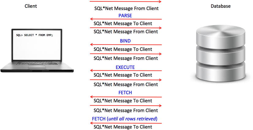
Figure 2-2. “Under the covers” of a SELECT statement execution
The network round-trip between the client and the database for each call contributes to the overall response time of the statement. There is only one of each type of database call except for FETCH. As mentioned previously, Oracle needs to execute as many FETCH calls as necessary to retrieve and return all the rows required to satisfy your query.
A single FETCH call accesses one or more blocks of data from the buffer cache. Each time a block is accessed, Oracle takes rows from the block and returns them to the client in one round-trip. The number of rows that are returned is a configurable setting called arraysize. The arraysize is the number of rows to be transmitted in a single network round-trip, if possible. If the size of the rows is too large to fit in a single packet, Oracle breaks up the rows into multiple packets, but even then, only a single FETCH call is needed to provide the specified number of rows.
The arraysize setting is set programmatically; how it is accomplished depends on which calling application environment you use. In SQL*Plus, in which the default arraysize is 15, you change the arraysize setting using the command SET ARRAYSIZE n. The JDBC default is ten and may be changed using ((OracleConnection)conn).setDefaultRowPrefetch (n). Make sure to discover your application’s arraysize setting and increase it as necessary. The benefit to having a larger arraysize is twofold: reduction of FETCH calls and reduction of network round-trips. It may not seem like much, but the impact can be quite stunning. Listing 2-16 demonstrates how logical reads for the same query are reduced simply by changing arraysize. Note that logical reads are labeled as buffers in the autotrace output.
Listing 2-16. How the arraysize Setting Affects Logical Reads
SQL> set arraysize 15
SQL>
SQL> set autotrace traceonly statistics
SQL>
SQL> select * from order_items ;

Statistics
----------------------------------------------------------
          0  recursive calls
          0  db block gets
         52  consistent gets
          0  physical reads
          0  redo size
      18815  bytes sent via SQL*Net to client
        865  bytes received via SQL*Net from client
         46  SQL*Net roundtrips to/from client
          0  sorts (memory)
          0  sorts (disk)
        664  rows processed

SQL>
SQL> set arraysize 45
SQL> /

Statistics
----------------------------------------------------------
          0  recursive calls
          0  db block gets
         22  consistent gets
          0  physical reads
          0  redo size
      15026  bytes sent via SQL*Net to client
        535  bytes received via SQL*Net from client
         16  SQL*Net roundtrips to/from client
          0  sorts (memory)
          0  sorts (disk)
        664  rows processed
Even for this small result set of 664 rows, the difference that increasing the arraysize setting produces is clearly visible. I increased the setting from 15 to 45, reduced the logical reads from 52 to 22, and reduced the number of network round-trips from 46 to 16! This change had nothing to do with the SQL statement and everything to do with how Oracle was able to access and return the rows. This is just one more example of how understanding how things work can help you to help Oracle use less resources and time to do what you ask of it.
SQL Execution: Putting It All Together
Now that I’ve covered the details, I’m ready to put together the whole picture of how a SQL statement executes. Figure 2-3 shows the steps that are involved when a SQL statement executes.
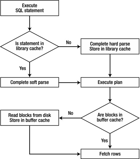
Figure 2-3. Overview of steps that occur when a SQL statement is executed
This is a simplified view, but it encapsulates the view of the process. From a big-picture perspective, every query must complete PARSE, EXECUTE, and FETCH steps. Data Manipulation Language (DML) statements (INSERT, UPDATE, DELETE) only need to parse and execute. In addition to these steps, statements that use bind variables also include a step to read the bind values as part of the parse component.
Summary
Understanding how SQL executes enables you to write it more effectively. The optimizer is at the heart of every SQL statement you write; writing SQL with the optimizer in mind helps you more than you can imagine. On this point, I’ll ask you to trust me for now. I can assure you that understanding the optimizer has been one of the most beneficial pieces of knowledge I’ve gained, so don’t get frustrated if you’re just itching to start looking at syntax and specific SQL code. What you end up with by the end of this journey is well worth it.
At this point, I hope you feel more comfortable with at least some of the key parts of Oracle’s architecture that are involved in the execution of the SQL you send to the database. You should also have a flavor for the power of statistics and how they are used by the optimizer. It is outside the scope of this book to go into more detail about this topic, but I highly recommend picking up Jonathan Lewis’s Cost-Based Oracle Fundamentals (Apress 2006) if you really want to take a deep dive into this subject matter. The more you know, the better equipped you’ll be to write SQL that works with the optimizer and not against it.
In the next chapter, I cover the access and join methods the optimizer can choose, and review numerous examples of how and why the optimizer does what it does. What I’ve covered so far has built the foundation for what I cover next, and each chapter continues to add to this foundation. The goal is to shed some light on the black box into which you’ve been throwing SQL and to help you develop an enriched perspective on the importance of what’s under the covers of Oracle—in particular, the optimizer—and how to interact properly with it.