
![]()
SQL Execution Plans
You’ve seen quite a few execution plans in the first chapters of this book, but in this chapter I go into detail about how to produce and read plans correctly. I’ve built the foundation of knowledge you need to understand the most common operations you’ll see used in execution plans, but now you need to put this knowledge into practice.
By the end of this chapter, I want you to feel confident that you can break down even the most complex execution plan and understand how any SQL statement you write is being executed. With the prevalence of development tools such as SQL Developer, SQL Navigator, and TOAD (just to name a few), which can produce explain plan output (which is simply the estimated execution plan), it is fairly easy to generate explain plan output. What isn’t as easy is to get execution plan output. You may be wondering what the difference is between an explain plan and an execution plan. As you’ll see in this chapter, there can be a significant difference. I’ll walk through the differences between explain plan output and actual execution plan information. You’ll learn how to compare the estimated plans with the actual plans, and how to interpret any differences that are present. This is “where the rubber meets the road,” as race car drivers would say.
Explain Plan
The EXPLAIN PLAN statement is used to display the plan operations chosen by the optimizer for a SQL statement. The first thing I want to clarify is that when you have EXPLAIN PLAN output, you have the estimated execution plan that should be used when the SQL statement is actually executed. You do not have the actual execution plan and its associated row-source execution statistics. You have estimates only—not the real thing. Throughout this chapter, I make the distinction between actual and estimated plan output by referring to estimated information as explain plan output and calling actual information as execution plan output.
Using Explain Plan
When using EXPLAIN PLAN to produce the estimated execution plan for a query, the output shows the following:
- Each of the tables referred to in the SQL statement
- The access method used for each table
- The join methods for each pair of joined row sources
- An ordered list of all operations to be completed
- A list of predicate information related to steps in the plan
- For each operation, the estimates for number of rows and bytes manipulated by that step
- For each operation, the computed cost value
- If applicable, information about partitions accessed
- If applicable, information about parallel execution
Listing 6-1 shows how to create and display the explain plan output for a query that joins five tables.
Listing 6-1. EXPLAIN PLAN Example
SQL> explain plan for
  2  select e.last_name || ', ' || e.first_name as full_name,
  3         e.phone_number, e.email, e.department_id,
  4         d.department_name, c.country_name, l.city, l.state_province,
  5         r.region_name
  6    from hr.employees e, hr.departments d, hr.countries c,
  7         hr.locations l, hr.regions r
  8   where e.department_id = d.department_id
  9     and d.location_id = l.location_id
 10     and l.country_id = c.country_id
 11     and c.region_id = r.region_id;

Explained.

SQL>select * from table(dbms_xplan.display(format=>'BASIC +COST +PREDICATE'));

PLAN_TABLE_OUTPUT
----------------------------------------------------------------------------
Plan hash value: 2352397467

-------------------------------------------------------------------------
| Id  | Operation                        | Name            | Cost (%CPU)|
-------------------------------------------------------------------------
|   0 | SELECT STATEMENT                 |                 |     3   (0)|
|   1 |  NESTED LOOPS                    |                 |            |
|   2 |   NESTED LOOPS                   |                 |     3   (0)|
|   3 |    NESTED LOOPS                  |                 |     3   (0)|
|   4 |     NESTED LOOPS                 |                 |     3   (0)|
|   5 |      NESTED LOOPS                |                 |     3   (0)|
|   6 |       TABLE ACCESS FULL          | EMPLOYEES       |     3   (0)|
|   7 |       TABLE ACCESS BY INDEX ROWID| DEPARTMENTS     |     0   (0)|
|*  8 |        INDEX UNIQUE SCAN         | DEPT_ID_PK      |     0   (0)|
|   9 |      TABLE ACCESS BY INDEX ROWID | LOCATIONS       |     0   (0)|
|* 10 |       INDEX UNIQUE SCAN          | LOC_ID_PK       |     0   (0)|
|* 11 |     INDEX UNIQUE SCAN            | COUNTRY_C_ID_PK |     0   (0)|
|* 12 |    INDEX UNIQUE SCAN             | REG_ID_PK       |     0   (0)|
|  13 |   TABLE ACCESS BY INDEX ROWID    | REGIONS         |     0   (0)|
-------------------------------------------------------------------------

Predicate Information (identified by operation id):
---------------------------------------------------

   8 - access("E"."DEPARTMENT_ID"="D"."DEPARTMENT_ID")
  10 - access("D"."LOCATION_ID"="L"."LOCATION_ID")
  11 - access("L"."COUNTRY_ID"="C"."COUNTRY_ID")
  12 - access("C"."REGION_ID"="R"."REGION_ID")
For this example, I used the EXPLAIN PLAN command to generate the explain plan content. I could have used AUTOTRACE instead to automate the steps to generate a plan so that all you have to do is turn on AUTOTRACE (using the TRACEONLY EXPLAIN option) and execute a query. The plan is generated and the output is displayed all in one step. In this example, I use the dbms_xplan.display function to display the output instead (I discuss dbms_xplan in more detail shortly). When using either method to generate a plan, neither the EXPLAIN PLAN command nor the SET AUTOTRACE TRACEONLY EXPLAIN option actually executes the query. It only generates the plan that is estimated to be executed. The development tool you use (SQL Developer, TOAD, and so forth) should also have an option to generate explain plans. I may be a bit old-fashioned, but I find the text output often easier to read than the semigraphical trees some of these common development tools use. I don’t particularly need or care to see any little graphical symbols, so I’m very happy with text output without any of the extra icons and such. But, don’t feel you have to generate explain plans using these methods if you prefer to use your tool.
The Plan Table
The information you see in explain plan output is generated by the EXPLAIN PLAN command and is stored in a table named PLAN_TABLE by default. The AUTOTRACE command calls the display function from the supplied package named dbms_xplan to format the output automatically. I executed the query manually using dbms_xplan when using EXPLAIN PLAN without turning on AUTOTRACE. For reference, Listing 6-2 shows the table description for the Oracle version 12c PLAN_TABLE.
Listing 6-2. PLAN_TABLE
SQL> desc plan_table
 Name                          Null?    Type
 ----------------------------- -------- ------------------
 STATEMENT_ID                           VARCHAR2(30)
 PLAN_ID                                NUMBER
 TIMESTAMP                              DATE
 REMARKS                                VARCHAR2(4000)
 OPERATION                              VARCHAR2(30)
 OPTIONS                                VARCHAR2(255)
 OBJECT_NODE                            VARCHAR2(128)
 OBJECT_OWNER                           VARCHAR2(30)
 OBJECT_NAME                            VARCHAR2(30)
 OBJECT_ALIAS                           VARCHAR2(65)
 OBJECT_INSTANCE                        NUMBER(38)
 OBJECT_TYPE                            VARCHAR2(30)
 OPTIMIZER                              VARCHAR2(255)
 SEARCH_COLUMNS                         NUMBER
 ID                                     NUMBER(38)
 PARENT_ID                              NUMBER(38)
 DEPTH                                  NUMBER(38)
 POSITION                               NUMBER(38)
 COST                                   NUMBER(38)
 CARDINALITY                            NUMBER(38)
 BYTES                                  NUMBER(38)
 OTHER_TAG                              VARCHAR2(255)
 PARTITION_START                        VARCHAR2(255)
 PARTITION_STOP                         VARCHAR2(255)
 PARTITION_ID                           NUMBER(38)
 OTHER                                  LONG
 OTHER_XML                              CLOB
 DISTRIBUTION                           VARCHAR2(30)
 CPU_COST                               NUMBER(38)
 IO_COST                                NUMBER(38)
 TEMP_SPACE                             NUMBER(38)
 ACCESS_PREDICATES                      VARCHAR2(4000)
 FILTER_PREDICATES                      VARCHAR2(4000)
 PROJECTION                             VARCHAR2(4000)
 TIME                                   NUMBER(38)
 QBLOCK_NAME                            VARCHAR2(30)
I’m not going to review every column listed, but I wanted to provide a table description from which you can do further study if you desire. You can find more information in the Oracle documentation.
The columns from PLAN_TABLE shown in the explain plan output in Listing 6-1 are only a few of the columns from the table. One of the nice things about the dbms_xplan.display function is that it has intelligence built in so that it displays the appropriate columns based on the specific plan generated for each SQL statement. For example, if the plan used partition operations, the PARTITION_START, PARTITION_STOP, and PARTITION_ID columns would appear in the display. The ability of dbms_xplan.display to determine automatically the columns that should be shown is a super feature that beats using the old do-it-yourself query against the PLAN_TABLE hands down.
The columns shown in the display for the example query plan are ID, OPERATION, OPTIONS, OBJECT_NAME, COST, ACCESS_PREDICATES, and FILTER_PREDICATES. These are the columns displayed based on the use of the format parameter of 'BASIC +COST +PREDICATE'. Table 6-1 provides a brief definition of each of these common columns.
Table 6-1. Most Commonly Used PLAN_TABLE Columns
| Column | Description |
|---|---|
| ID | Unique number assigned to each step |
| OPERATION | Internal operation performed by the step |
| OPTIONS | Additional specification for the operation column (appended to OPERATION) |
| OBJECT_NAME | Name of the table or index |
| COST | Weighted cost value for the operation as determined by the optimizer |
| ACCESS_PREDICATES | Conditions used to locate rows in an access structure (typically an index) |
| FILTER_PREDICATES | Conditions used to filter rows after they have been accessed |
One of the columns from the PLAN_TABLE that is not displayed in the plan display output when using the dbms_xplan.display function is the PARENT_ID column. Instead of displaying this column value, the output is indented to provide a visual cue for the parent–child relationships within the plan. I think it is helpful to include the PARENT_ID column value as well, for clarity, but you have to write your own query against the PLAN_TABLE to produce the output to include that column if you want it. I use a script from Randolf Geist’s blog (http://oracle-randolf.blogspot.com/2011/12/extended-displaycursor-with-rowsource.html) that adds the PARENT_ID column to the dbms_xplan.display output. Another column, Ord, has also been added to indicate the execution order of the operations. The script provides lots of other additional output that you can use as well. I recommend reading Geist’s full blog post and downloading the script for your own use. Although I have elided some of the output available, Listing 6-3 shows using this script for our previous query executed for Listing 6-1. Note that I had to execute the query (not just use EXPLAIN PLAN) and capture SQL_ID to supply the correct input parameters to the script (again, see Geist’s blog for usage details).
Listing 6-3. Displaying the PARENT_ID and Ord columns using the xpext.sql script
SQL>@xpext cqbz6zv6tu5g3 0 "BASIC +PREDICATE"
EXPLAINED SQL STATEMENT:
------------------------
select e.last_name | ', ' || e.first_name as full_name,
     e.phone_number, e.email, e.department_id,
d.department_name, c.country_name, l.city, l.state_province,
r.region_name   from hr.employees e, hr.departments d, hr.countries c,
      hr.locations l, hr.regions r  where e.department_id =
d.department_id    and d.location_id = l.location_id    and
l.country_id = c.country_id    and c.region_id = r.region_id

Plan hash value: 2352397467

-----------------------------------------------------------------------------------
| Id  | Pid | Ord | Operation                        | Name            |E-Rows*Sta|
-----------------------------------------------------------------------------------
|   0 |     |  14 | SELECT STATEMENT                 |                 |          |
|   1 |   0 |  13 |  NESTED LOOPS                    |                 |          |
|   2 |   1 |  11 |   NESTED LOOPS                   |                 |      106 |
|   3 |   2 |   9 |    NESTED LOOPS                  |                 |      106 |
|   4 |   3 |   7 |     NESTED LOOPS                 |                 |      106 |
|   5 |   4 |   4 |      NESTED LOOPS                |                 |      106 |
|   6 |   5 |   1 |       TABLE ACCESS FULL          | EMPLOYEES       |      107 |
|   7 |   5 |   3 |       TABLE ACCESS BY INDEX ROWID| DEPARTMENTS     |      107 |
|*  8 |   7 |   2 |        INDEX UNIQUE SCAN         | DEPT_ID_PK      |      107 |
|   9 |   4 |   6 |      TABLE ACCESS BY INDEX ROWID | LOCATIONS       |      106 |
|* 10 |   9 |   5 |       INDEX UNIQUE SCAN          | LOC_ID_PK       |      106 |
|* 11 |   3 |   8 |     INDEX UNIQUE SCAN            | COUNTRY_C_ID_PK |      106 |
|* 12 |   2 |  10 |    INDEX UNIQUE SCAN             | REG_ID_PK       |      106 |
|  13 |   1 |  12 |   TABLE ACCESS BY INDEX ROWID    | REGIONS         |      106 |
-----------------------------------------------------------------------------------

Predicate Information (identified by operation id):
---------------------------------------------------
   8 - access("E"."DEPARTMENT_ID"="D"."DEPARTMENT_ID")
  10 - access("D"."LOCATION_ID"="L"."LOCATION_ID")
  11 - access("L"."COUNTRY_ID"="C"."COUNTRY_ID")
  12 - access("C"."REGION_ID"="R"."REGION_ID")
PARENT_ID (shown in the Pid column in Listing 6-3) is helpful because operations in a plan are easiest to read if you keep in mind the parent–child relationships involved in the plan. Each step in the plan has from zero to two children. If you break down the plan into smaller chunks of parent–child groupings, it makes it easier to read and understand.
Breaking Down the Plan
When learning how to read plan output, it is important to start with an understanding of how the plan is organized. In this section, I help you understand the relationships between various elements of a plan and how to break the plan into smaller groups of related operations. Reading a plan with understanding can be more difficult than it may seem, particularly if the plan is long. But, by breaking the plan apart, it’s often easier to put it back together in a way that makes more sense to you.
Let’s start by considering the relationships between various plan operations. In the example plan, you have operations with zero, one, and two children. A full table scan operation, for example, doesn’t have any children. See the line for ID=5 in Listing 6-3. Another example of an operation with zero children is line 3. If you glance down the Pid column, you can see that neither step 3 nor step 5 show up, which means these operations do not depend on any other operation to complete. Both operations are children of other operations, however, and they pass the data they access to their parent step. When an operation has no children, the Rows (CARDINALITY column in the PLAN_TABLE) estimate represents the number of rows that a single iteration of that operation acquires. This can be a bit confusing when the operation is providing rows to an iterative parent, but the estimate for the operation doesn’t indicate the total number of rows accessed in that step. The total is determined by the parent operation. I delve into this in more detail shortly.
The parent steps for steps 3 and 5—steps 2 and 4—are examples of single-child operations. In general, operations with only one child can be divided into three categories:
- Working operations, which receive a row set from the child operation and manipulate it further before passing it on to its parent.
- Pass-thru operations, which act simply as a pass-thru and don’t alter or manipulate the data from the child in any way. They basically serve to identify an operation characteristic. The VIEW operation is a good example of a pass-thru operation.
- Iterative operations, which indicate there are multiple executions of the child operation. You typically see the word ITERATOR, INLIST, or ALL in these types of operation names.
Both step 2 and step 4 are working operations. They take the row sets from their children (steps 3 and 5) and do some additional work. In step 2, the rowids returned from the index full scan are used to retrieve the DEPARTMENT table data blocks. In step 4, the rows returned from the full scan of the EMPLOYEES table are sorted in order by the join column.
Last, operations that have two children operate either iteratively or in succession. When the parent type is iterative, the child row sources are accessed such that for each row in row source A, B is accessed. For a parent operation that works on the children in succession, the first child row source is accessed followed by an access of the second row source. Join types such as NESTED LOOPS and MERGE JOIN are iterative, as is the FILTER operation. All other operations with two children work in succession on their child row sources.
The reason for this review is to highlight the importance of learning to take a divide-and-conquer approach to reading and understanding plan output. The larger and more complicated a plan looks, the harder it often is to find the key problem areas. If you learn to look for parent–child relationships in the plan output, and narrow your focus to smaller chunks of the plan, you’ll find it much easier to work with what you see.
Understanding How EXPLAIN PLAN Can Miss the Mark
One of the most frustrating things about EXPLAIN PLAN output is that it may not always match the plan that is used when the statement is actually executed, even when no objects referenced in the query change structurally in between. There are four things to keep in mind about using EXPLAIN PLAN that make it susceptible to producing plan output that doesn’t match the actual execution plan:
- EXPLAIN PLAN produces plans based on the environment at the moment you use it.
- EXPLAIN PLAN doesn’t consider the datatype of bind variables (all binds are VARCHAR2).
- EXPLAIN PLAN doesn’t “peek” at bind variable values.
- EXPLAIN PLAN only shows the original plan and not the final plan (this references a 12c feature called adaptive query optimization, which is covered in a later chapter).
For these reasons, as mentioned, it is very possible that EXPLAIN PLAN produces a plan that doesn’t match the plan that is produced when the statement is actually executed. Listing 6-4 demonstrates the second point about bind variable datatypes causing EXPLAIN PLAN not to match the actual execution plan.
Listing 6-4. EXPLAIN PLAN and Bind Variable Datatypes
SQL>-- Create a test table where primary key column is a string datatype
SQL> create table regions2
  2  (region_id  varchar2(10) primary key,
  3   region_name varchar2(25));

Table created.

SQL>
SQL>-- Insert rows into the test table
SQL> insert into regions2
  2  select * from regions;

4 rows created.

SQL>
SQL>-- Create a variable and set its value
SQL> variable regid number
SQL> exec :regid := 1

PL/SQL procedure successfully completed.

SQL>
SQL>-- Get explain plan for the query
SQL> explain plan for select /* DataTypeTest */ *
  2  from regions2
  3  where region_id = :regid;

Explained.
SQL> select * from table(dbms_xplan.display(format=>'BASIC +COST +PREDICATE'));

Plan hash value: 2358393386

----------------------------------------------------------------
| Id  | Operation                   | Name        | Cost (%CPU)|
----------------------------------------------------------------
|   0 | SELECT STATEMENT            |             |     1   (0)|
|   1 |  TABLE ACCESS BY INDEX ROWID| REGIONS2    |     1   (0)|
|*  2 |   INDEX UNIQUE SCAN         | SYS_C009951 |     1   (0)|
----------------------------------------------------------------

Predicate Information (identified by operation id):
---------------------------------------------------

   2 - access("REGION_ID"=:REGID)

SQL>
SQL>-- Execute the query
SQL> select /* DataTypeTest */ *
  2  from regions2
  3  where region_id = :regid;

REGION_ID  REGION_NAME
---------- -------------------------
1          Europe

SQL>
SQL>-- Review the actual execution plan
SQL> select * from table(dbms_xplan.display_cursor(null,null,format=>'BASIC +COST +PREDICATE'));

EXPLAINED SQL STATEMENT:
------------------------
select /* DataTypeTest */ * from regions2 where region_id = :regid

Plan hash value: 670750275

---------------------------------------------------
| Id  | Operation         | Name     | Cost (%CPU)|
---------------------------------------------------
|   0 | SELECT STATEMENT  |          |     3 (100)|
|*  1 |  TABLE ACCESS FULL| REGIONS2 |     3   (0)|
---------------------------------------------------

Predicate Information (identified by operation id):
---------------------------------------------------
   1 - filter(TO_NUMBER("REGION_ID")=:REGID)
Did you notice how the explain plan output indicated that the primary key index would be used but the actual plan really used a full table scan? The reason why is clearly shown in the Predicate Information section. In the explain plan output, the predicate is "REGION_ID"=:REGID, but in the actual plan, the predicate shows TO_NUMBER("REGION_ID")=:REGID. This demonstrates how EXPLAIN PLAN doesn’t consider the datatype of a bind variable and assumes all bind variables are string types. For EXPLAIN PLAN, the datatypes were considered to be the same (both strings). However, the datatypes were considered when the plan was prepared for the actual execution of the statement, and Oracle implicitly converted the string datatype for the REGION_ID column to a number to match the bind variable datatype (NUMBER). This is expected behavior in that, when datatypes being compared don’t match, Oracle always attempts to convert the string datatype to match the nonstring datatype. By doing so in this example, the TO_NUMBER function caused the use of the index to be disallowed. This is another expected behavior to keep in mind: The predicate must match the index definition exactly or else the index is not used.
If you are testing this statement in your development environment and use the explain plan output to confirm that the index is being used, you are wrong. From the explain plan output, it appears that the plan is using the index, as you would expect, but when the statement is actually executed, performance is likely to be unsatisfactory because of the full table scan that really occurs.
Another issue with using explain plan output as your sole source for testing is that you never get a true picture of how the statement uses resources. Estimates are just that—estimates. To confirm the behavior of the SQL and to make intelligent choices about whether the statement will provide optimal performance, you need to look at actual execution statistics. I cover the details of how to capture and interpret actual execution statistics shortly.
Before I dive further into capturing actual execution plan data, I want to make sure you are comfortable with reading a plan. I’ve already discussed the importance of the PARENT_ID column in making it easier for you to break down a long, complex plan into smaller, more manageable sections. Breaking down a plan into smaller chunks helps you read it, but you need to know how to approach reading a whole plan from start to finish.
There are three ways that help you read and understand any plan: (1) learn to identify and separate parent–child groupings (I discussed this earlier in the “Breaking Down the Plan” section), (2) learn the order in which the plan operations execute, and (3) learn to read the plan in narrative form. I learned to do these three things so that when I look at a plan, my eyes move through the plan easily and I notice possible problem areas quickly. The process can be frustrating and you may be a bit slow at first, but given time and practice, this activity becomes second nature.
Let’s start with execution order. The plan is displayed in order by the sequential ID of operations. However, the order in which each operation executes isn’t accomplished in a precise top-down fashion. To be precise, the first operation executed in an execution plan is actually the first operation from the top of the execution plan that has no child operations. In most cases, using the visual cues of the indentation of the operations, you can scan a plan quickly and look for the operations that are the most indented. The operation that is most indented is usually the first operation that is executed. If there are multiple operations at that same level, the operations are executed in a top-down order. But, in some cases, the visual cue to look for the first most-indented operation won’t work and you have to remember simply to find the first operation from the top of the execution plan that has no child operations.
For reference, I relist the example plan here in Listing 6-5 so that you don’t have to flip back a few pages to the original example in Listing 6-1.
Listing 6-5. EXPLAIN PLAN Example (Repeated)
-------------------------------------------------------------------------
| Id  | Operation                        | Name            | Cost (%CPU)|
-------------------------------------------------------------------------
|   0 | SELECT STATEMENT                 |                 |     3   (0)|
|   1 |  NESTED LOOPS                    |                 |            |
|   2 |   NESTED LOOPS                   |                 |     3   (0)|
|   3 |    NESTED LOOPS                  |                 |     3   (0)|
|   4 |     NESTED LOOPS                 |                 |     3   (0)|
|   5 |      NESTED LOOPS                |                 |     3   (0)|
|   6 |       TABLE ACCESS FULL          | EMPLOYEES       |     3   (0)|
|   7 |       TABLE ACCESS BY INDEX ROWID| DEPARTMENTS     |     0   (0)|
|*  8 |        INDEX UNIQUE SCAN         | DEPT_ID_PK      |     0   (0)|
|   9 |      TABLE ACCESS BY INDEX ROWID | LOCATIONS       |     0   (0)|
|* 10 |       INDEX UNIQUE SCAN          | LOC_ID_PK       |     0   (0)|
|* 11 |     INDEX UNIQUE SCAN            | COUNTRY_C_ID_PK |     0   (0)|
|* 12 |    INDEX UNIQUE SCAN             | REG_ID_PK       |     0   (0)|
|  13 |   TABLE ACCESS BY INDEX ROWID    | REGIONS         |     0   (0)|
-------------------------------------------------------------------------

Predicate Information (identified by operation id):
---------------------------------------------------
   8 - access("E"."DEPARTMENT_ID"="D"."DEPARTMENT_ID")
  10 - access("D"."LOCATION_ID"="L"."LOCATION_ID")
  11 - access("L"."COUNTRY_ID"="C"."COUNTRY_ID")
  12 - access("C"."REGION_ID"="R"."REGION_ID")
At a glance, you can see that lines 6 and 8 are the most deeply indented. Line 6 executes first, then line 8 executes next and passes the rowids from the index unique scan to its parent (line 7). Steps continue to execute from the most indented to the least indented, with each step passing row-source data to its parent until all steps complete. To help see the execution order more clearly, Listing 6-6 repeats a portion of the output from Listing 6-3 for the xpext.sql script, which shows the operations in execution order.
Listing 6-6. Plan Operations Displayed in Execution Order (from xpext.sql in Listing 6-3)
------------------------------------------------------------------------
| Id  | Pid | Ord | Operation                        | Name            |
------------------------------------------------------------------------
|   6 |   5 |   1 |       TABLE ACCESS FULL          | EMPLOYEES       |
|   8 |   7 |   2 |        INDEX UNIQUE SCAN         | DEPT_ID_PK      |
|   7 |   5 |   3 |       TABLE ACCESS BY INDEX ROWID| DEPARTMENTS     |
|   5 |   4 |   4 |      NESTED LOOPS                |                 |
|  10 |   9 |   5 |       INDEX UNIQUE SCAN          | LOC_ID_PK       |
|   9 |   4 |   6 |      TABLE ACCESS BY INDEX ROWID | LOCATIONS       |
|   4 |   3 |   7 |     NESTED LOOPS                 |                 |
|  11 |   3 |   8 |     INDEX UNIQUE SCAN            | COUNTRY_C_ID_PK |
|   3 |   2 |   9 |    NESTED LOOPS                  |                 |
|  12 |   2 |  10 |    INDEX UNIQUE SCAN             | REG_ID_PK       |
|   2 |   1 |  11 |   NESTED LOOPS                   |                 |
|  13 |   1 |  12 |   TABLE ACCESS BY INDEX ROWID    | REGIONS         |
|   1 |   0 |  13 |  NESTED LOOPS                    |                 |
|   0 |     |  14 | SELECT STATEMENT                 |                 |
------------------------------------------------------------------------
I often use an analogy between parent–child relationships in a plan and real life parent–child relationships. A real child doesn’t just spontaneously combust into being; a parent is required to “instantiate” the child into being. But, as most any parent will tell you, one of the greatest things about kids is that (sometimes) you can get them to do work for you. This applies to parent–child operations in a plan. The child takes direction from its parent and goes to do a piece of work. When the child completes that work, it reports back to the parent with the result. So, even though an index operation occurs before its parent (for example, step 6 executes before its parent in step 5), the child doesn’t have meaning or existence without its parent. This is why it’s important always to keep parent–child relationships in mind, because they help make sense of the execution order.
Access and Filter Predicates
One of the most helpful sections of the explained output is the section named Predicate Information. In this section, the ACCESS_PREDICATES and FILTER_PREDICATES columns are displayed. These columns are associated with a line (denoted by the ID column) in the list of plan operations. Notice that for each plan operation that has an access or filter predicate associated with it, there is an asterisk (*)next to the ID. When you see the asterisk, you know to look for that ID number in the Predicate Information section to see which predicate (condition in the WHERE clause) is related to that operation. Using this information, you can confirm that columns are used correctly (or not) for index access and also you can determine where a condition was filtered.
An access predicate is either going to be an index operation or a join operation. An access predicate is simply a more direct way to access the data by retrieving only the rows in the table that match a condition in the WHERE clause or when matching the columns that join two tables. Filter predicates are a less exact way to retrieve the data in that, when a filter predicate is applied, all rows in the current row source must be checked to determine whether they pass the filter. On the other hand, an access predicate only places rows into a resulting row source when there is an exact match. Thus, access predicates are often thought of as more efficient because they typically only gather rows that match the condition vs. hitting all the rows and throwing away what doesn’t match.
Filtering late is a common performance inhibitor. For example, if you want to move a pile of 100 rocks from the front yard to your backyard but only need rocks that weigh 5 to 10 pounds, would you move all 100 rocks and then remove the ones you need? Or would you simply move those that are the correct weight? In general, you want to take only the rocks you need, right?
Using the filter predicate information can help you verify that unneeded rows are filtered out of your result set as early as possible in the plan. Just like it doesn’t make much sense to carry a whole bunch of extra rocks to the backyard, it doesn’t make much sense to carry rows through a whole set of plan operations that ultimately are not included in the final result set. Use the filter information to verify that each condition is applied as early in the plan as possible. If a filter is applied too late, you can adjust your SQL or take other steps (such as verifying that statistics are up to date) to ensure your plan isn’t working harder than it needs to.
Reading the Plan as a Narrative
Last, learning to read the plan as if it is a narrative can be extremely helpful. For many people, converting the set of plan operations into a paragraph of text facilitates understanding how the plan executes better than any other method. Let’s convert the example plan into a narrative and see whether it makes it easier for you to read and understand. The following paragraph is a sample narrative for the example plan.
To produce the result set for this SELECT statement, rows from the DEPARTMENTS table are accessed using a full scan of the index on the DEPARTMENTS.LOCATION_ID column. Using a full scan of the LOCATIONS table, rows are retrieved and sorted by LOCATION_ID and then merged with the rows from DEPARTMENTS to produce a joined result set of matching rows containing both DEPARTMENTS and LOCATIONS data. This row set, which we call DEPT_LOC, is joined to the COUNTRIES table and matches iteratively one row from DEPT_LOC using COUNTRY_ID to find a matching row in COUNTRIES. This result set, which we call DEPT_LOC_CTRY, now contains data from DEPARTMENTS, LOCATIONS, and COUNTRIES, and is hashed into memory and matched with the REGIONS table data using REGION_ID. This result set, DEPT_LOC_CTRY_REG, is hashed into memory and matched with the EMPLOYEES table using DEPARTMENT_ID to produce the final result set of rows.
To produce this narrative, I simply walk through the steps of the plan in execution order and write out the description of the steps and how they link (join) to each other. I progress through each set of parent–child operations until all the steps are complete. You may find that creating a narrative helps you grasp the overall plan with a bit more clarity. For more complex plans, you may find that breaking out just a few key portions of the whole plan and writing them out in narrative form will help you understand the flow of operations more completely. The key is to use the narrative to help make better sense of the plan. If you find it harder to do this, then just stick with the plan as it is. But, taking time to learn to convert a plan into a narrative form is a good skill to learn, because it can help you describe what your query is doing in a way that doesn’t require anyone even looking at plan output. It’s similar to giving verbal directions on how to get to the nearest shopping mall. You don’t necessarily have to have the map to be able to get from point A to point B.
Execution Plans
The actual execution plan for a SQL statement is produced when a statement is executed. After the statement is hard parsed, the plan that is chosen is stored in the library cache for later reuse. The plan operations can be viewed by querying V$SQL_PLAN, which has basically the same definition as PLAN_TABLE, except that it has several columns that contain the information on how to identify and find the statement in the library cache. These additional columns are ADDRESS, HASH_VALUE, SQL_ID, PLAN_HASH_VALUE, CHILD_ADDRESS, and CHILD_NUMBER. You can find any SQL statement using one or more of these values.
Viewing Recently Generated SQL
Listing 6-7 shows a query against V$SQL for recently executed SQL for the SCOTT user and the identifying values for each column.
Listing 6-7. V$SQL Query to Get Recently Executed SQL
SQL>select /* recentsql */ sql_id, child_number,
  2         hash_value, address, executions, sql_text
  3    from v$sql
  4   where parsing_user_id = (select user_id
  5                             from all_users
  6                             where username = 'SCOTT')
  7     and command_type in (2,3,6,7,189)
  8     and UPPER(sql_text) not like UPPER('%recentsql%'),

SQL_ID        CHILD_NUMBER HASH_VALUE ADDRESS  EXECUTIONS SQL_TEXT
------------- ------------ ---------- -------- ---------- --------------------
g5wp7pwtq4kwp            0  862079893 3829AE54          1 select * from emp
1gg46m60z7k2p            0 2180237397 38280AD0          1 select * from bonus
4g0qfgmtb7z70            0 4071881952 38281D68          1 select * from dept

3 rows selected.
After connecting as user SCOTT, you execute the three queries shown. Then, when you run the query against V$SQL, you can see they are now loaded into the library cache and each has identifiers associated with it. The SQL_ID and CHILD_NUMBER columns contain the identifying information that you’ll use most often to retrieve a statement’s plan and execution statistics.
Viewing the Associated Execution Plan
There are several ways to view the execution plan for any SQL statement that has been previously executed and still remains in the library cache. The easiest way is to use the dbms_xplan.display_cursor function. Listing 6-8 shows how to use dbms_xplan.display_cursor to show the execution plan for the most recently executed SQL statement (note that some output columns have been elided for brevity).
Listing 6-8. Using dbms_xplan.display_cursor
SQL>select /*+ gather_plan_statistics */ empno, ename from scott.emp where ename = 'KING' ;

     EMPNO ENAME
---------- ----------
      7839 KING
SQL>
SQL>set serveroutput off
SQL>select * from table(dbms_xplan.display_cursor(null,null,'ALLSTATS LAST'));

PLAN_TABLE_OUTPUT
---------------------------------------------------------------------------
SQL_ID  2dzsuync8upv0, child number 0
-------------------------------------
select empno, ename from scott.emp where ename = 'KING'

Plan hash value: 3956160932

-----------------------------------------------------------------------
| Id  | Operation         | Name | Starts | E-Rows | A-Rows | Buffers |
-----------------------------------------------------------------------
|   0 | SELECT STATEMENT  |      |      1 |        |      1 |       8 |
|*  1 |  TABLE ACCESS FULL| EMP  |      1 |      1 |      1 |       8 |
-----------------------------------------------------------------------

Predicate Information (identified by operation id):
---------------------------------------------------

   1 - filter("ENAME"='KING')
First, note the use of the gather_plan_statistics hint in the query. To capture row-source execution statistics for the plan, you must tell Oracle to gather this information as the statement executes. The row-source execution statistics include the number of rows, number of consistent reads, number of physical reads, number of physical writes, and the elapsed time for each operation on a row. This information can be gathered using this hint on a statement-by-statement basis, or you can set the STATISTICS_LEVEL instance parameter to ALL. Capturing these statistics does add some overhead to the execution of a statement, and so you may not want to have it “always on.” The hint allows you to use it when you need to—and only for the individual statements you choose. The presence of this hint collects the information and shows it in the Starts, A-Rows, and Buffers columns. Listing 6-9 shows how the plan output appears if you don’t use the hint (or set the parameter value to ALL).
Listing 6-9. Using dbms_xplan.display_cursor without the gather_plan_statistics hint
SQL>select ename from scott.emp where ename = 'KING' ;

ENAME
----------
KING

SQL>select * from table(dbms_xplan.display_cursor(null,null,'ALLSTATS LAST'));

PLAN_TABLE_OUTPUT
------------------------------------------------------------------------
SQL_ID  32rvc78ypwhn8, child number 0
-------------------------------------
select ename from scott.emp where ename = 'KING'

Plan hash value: 3956160932

-------------------------------------------
| Id  | Operation         | Name | E-Rows |
-------------------------------------------
|   0 | SELECT STATEMENT  |      |        |
|*  1 |  TABLE ACCESS FULL| EMP  |      1 |
-------------------------------------------

Predicate Information (identified by operation id):
---------------------------------------------------

   1 - filter("ENAME"='KING')

Note
-----
   - Warning: basic plan statistics not available. These are only collected when:
    * hint 'gather_plan_statistics' is used for the statement or
    * parameter 'statistics_level' is set to 'ALL', at session or system level
As you can see, a note is displayed that indicates the plan statistics aren’t available and it tells you what to do to collect them.
Collecting the Plan Statistics
The plan operations shown when no plan statistics are available is essentially the same as the output from EXPLAIN PLAN. To get to the heart of how well the plan worked, you need the plan’s row-source execution statistics. These values tell you what actually happened for each operation in the plan. These data are pulled from the V$SQL_PLAN_STATISTICS view, which links each operation row for a plan to a row of statistics data. A composite view named V$SQL_PLAN_STATISTICS_ALL contains all the columns from V$SQL_PLAN plus the columns from V$SQL_PLAN_STATISTICS as well as a few additional columns containing information about memory usage. Listing 6-10 describes the V$SQL_PLAN_STATISTICS_ALL view columns.
Listing 6-10. The V$SQL_PLAN_STATISTICS_ALL View Description
SQL> desc v$sql_plan_statistics_all
 Name                                Null?    Type
 ----------------------------------- -------- ------------------------
 ADDRESS                                      RAW(8)
 HASH_VALUE                                   NUMBER
 SQL_ID                                       VARCHAR2(13)
 PLAN_HASH_VALUE                              NUMBER
 FULL_PLAN_HASH_VALUE                         NUMBER
 CHILD_ADDRESS                                RAW(8)
 CHILD_NUMBER                                 NUMBER
 TIMESTAMP                                    DATE
 OPERATION                                    VARCHAR2(30)
 OPTIONS                                      VARCHAR2(30)
 OBJECT_NODE                                  VARCHAR2(40)
 OBJECT#                                      NUMBER
 OBJECT_OWNER                                 VARCHAR2(30)
 OBJECT_NAME                                  VARCHAR2(30)
 OBJECT_ALIAS                                 VARCHAR2(65)
 OBJECT_TYPE                                  VARCHAR2(20)
 OPTIMIZER                                    VARCHAR2(20)
 ID                                           NUMBER
 PARENT_ID                                    NUMBER
 DEPTH                                        NUMBER
 POSITION                                     NUMBER
 SEARCH_COLUMNS                               NUMBER
 COST                                         NUMBER
 CARDINALITY                                  NUMBER
 BYTES                                        NUMBER
 OTHER_TAG                                    VARCHAR2(35)
 PARTITION_START                              VARCHAR2(64)
 PARTITION_STOP                               VARCHAR2(64)
 PARTITION_ID                                 NUMBER
 OTHER                                        VARCHAR2(4000)
 DISTRIBUTION                                 VARCHAR2(20)
 CPU_COST                                     NUMBER
 IO_COST                                      NUMBER
 TEMP_SPACE                                   NUMBER
 ACCESS_PREDICATES                            VARCHAR2(4000)
 FILTER_PREDICATES                            VARCHAR2(4000)
 PROJECTION                                   VARCHAR2(4000)
 TIME                                         NUMBER
 QBLOCK_NAME                                  VARCHAR2(30)
 REMARKS                                      VARCHAR2(4000)
 OTHER_XML                                    CLOB
 EXECUTIONS                                   NUMBER
 LAST_STARTS                                  NUMBER
 STARTS                                       NUMBER
 LAST_OUTPUT_ROWS                             NUMBER
 OUTPUT_ROWS                                  NUMBER
 LAST_CR_BUFFER_GETS                          NUMBER
 CR_BUFFER_GETS                               NUMBER
 LAST_CU_BUFFER_GETS                          NUMBER
 CU_BUFFER_GETS                               NUMBER
 LAST_DISK_READS                              NUMBER
 DISK_READS                                   NUMBER
 LAST_DISK_WRITES                             NUMBER
 DISK_WRITES                                  NUMBER
 LAST_ELAPSED_TIME                            NUMBER
 ELAPSED_TIME                                 NUMBER
 POLICY                                       VARCHAR2(10)
 ESTIMATED_OPTIMAL_SIZE                       NUMBER
 ESTIMATED_ONEPASS_SIZE                       NUMBER
 LAST_MEMORY_USED                             NUMBER
 LAST_EXECUTION                               VARCHAR2(10)
 LAST_DEGREE                                  NUMBER
 TOTAL_EXECUTIONS                             NUMBER
 OPTIMAL_EXECUTIONS                           NUMBER
 ONEPASS_EXECUTIONS                           NUMBER
 MULTIPASSES_EXECUTIONS                       NUMBER
 ACTIVE_TIME                                  NUMBER
 MAX_TEMPSEG_SIZE                             NUMBER
 LAST_TEMPSEG_SIZE                            NUMBER
 CON_ID                                       NUMBER
 CON_DBID                                     NUMBER
The columns containing the pertinent statistics information that relates to the output from dbms_xplan.display_cursor all begin with the prefix LAST_. When you use the format option of ALLSTATS LAST, the plan shows these column values for each row in the plan. So, for each operation, you know exactly how many rows it returns (LAST_OUTPUT_ROWS is shown in the A-Rows column), how many consistent reads occur (LAST_CR_BUFFER_GETS is shown in the Buffers column), how many physical reads occur (LAST_DISK_READS is shown in the Reads column), and the number of times a step is executed (LAST_STARTS is shown in the Starts column). There are several other columns that display, depending on the operations that take place, but these are the most common.
The dbms_xplan.display_cursor call signature is as follows:
FUNCTION DISPLAY_CURSOR RETURNS DBMS_XPLAN_TYPE_TABLE
 Argument Name                  Type                    In/Out Default?
 ------------------------------ ----------------------- ------ --------
 SQL_ID                         VARCHAR2                IN     DEFAULT
 CURSOR_CHILD_NO                NUMBER(38)              IN     DEFAULT
 FORMAT                         VARCHAR2                IN     DEFAULT
In the example from Listing 6-8, the three parameters used were SQL_ID => null, CURSOR_CHILD_NO => null, and FORMAT => ALLSTATS LAST. The use of nulls for the SQL_ID and CURSOR_CHILD_NO parameters indicates that the plan for the last executed statement should be retrieved. Therefore, you should be able to execute a statement, then execute the following:
select * from table(dbms_xplan.display_cursor(null,null,'ALLSTATS LAST'));
This gives you the plan output as shown in Listing 6-8.
![]() Caution You may have noticed that I executed the SQL*Plus command SET SERVEROUTPUT OFF before executing the call to dbms_xplan.display_cursor. This is a slight oddity that might catch you off-guard if you don’t know about it. Whenever you execute a statement and SERVEROUTPUT is ON, a call to dbms_output is executed implicitly. If you don’t use SERVEROUTPUT OFF, then the last statement executed is this dbms_output call. Using nulls for the first two parameters does not give you the SQL statement you executed, but instead attempts to give you the plan for the dbms_output call. Simply turning this setting to OFF stops the implicit call and ensures you get the plan for your most recently executed statement.
Caution You may have noticed that I executed the SQL*Plus command SET SERVEROUTPUT OFF before executing the call to dbms_xplan.display_cursor. This is a slight oddity that might catch you off-guard if you don’t know about it. Whenever you execute a statement and SERVEROUTPUT is ON, a call to dbms_output is executed implicitly. If you don’t use SERVEROUTPUT OFF, then the last statement executed is this dbms_output call. Using nulls for the first two parameters does not give you the SQL statement you executed, but instead attempts to give you the plan for the dbms_output call. Simply turning this setting to OFF stops the implicit call and ensures you get the plan for your most recently executed statement.
Identifying SQL Statements for Later Plan Retrieval
If you want to retrieve a statement that was executed in the past, you can retrieve the SQL_ID and CHILD_NUMBER from V$SQL as demonstrated in Listing 6-7. To simplify finding the correct statement identifiers, especially when I’m testing, I add a unique comment that identifies each statement I execute. Then, whenever I want to grab that plan from the library cache, all I have to do is query V$SQL to locate the statement text that includes the comment I used. Listing 6-11 shows an example of this and the query I use to subsequently find the statement I want.
Listing 6-11. Using a Comment to Identify a SQL Statement Uniquely
SQL>select /* KM-EMPTEST1 */ empno, ename
  2   from emp
  3  where job = 'MANAGER' ;

     EMPNO ENAME
---------- ----------
      7566 JONES
      7698 BLAKE
      7782 CLARK

SQL>select sql_id, child_number, sql_text
  2  from v$sql
  3  where sql_text like '%KM-EMPTEST1%';

SQL_ID        CHILD_NUMBER SQL_TEXT
------------- ------------ -------------------------------------------
9qu1dvthfcqsp            0 select /* KM-EMPTEST1 */     empno, ename
                               from emp where job = 'MANAGER'
a7nzwn3t522mt            0 select sql_id, child_number, sql_text from
                               v$sql where sql_text like '%KM-EMPTEST1%'

SQL>select * from table(dbms_xplan.display_cursor('9qu1dvthfcqsp',0,'ALLSTATS LAST'));

PLAN_TABLE_OUTPUT
----------------------------------------------------------------------------
SQL_ID  9qu1dvthfcqsp, child number 0
-------------------------------------
select /* KM-EMPTEST1 */ empno, ename  from emp where job = 'MANAGER'

Plan hash value: 3956160932

-----------------------------------------------------------------------
| Id  | Operation         | Name | Starts | E-Rows | A-Rows | Buffers |
-----------------------------------------------------------------------
|   0 | SELECT STATEMENT  |      |      1 |        |      3 |       8 |
|*  1 |  TABLE ACCESS FULL| EMP  |      1 |      3 |      3 |       8 |
-----------------------------------------------------------------------

Predicate Information (identified by operation id):
---------------------------------------------------

   1 - filter("JOB"='MANAGER')
Notice that when I query V$SQL, two statements show up. One is the SELECT statement I executed to find the entry in V$SQL and one is the query I executed. Although this series of steps gets the job done, I find it easier to automate the whole process into a single script. In this script, I find the statement I want in V$SQL by weeding out the query I’m running to find it and also by ensuring that I find the most recently executed statement that uses my identifying comment. Listing 6-12 shows the script I use in action.
Listing 6-12. Automating Retrieval of an Execution Plan for Any SQL Statement
SQL>select /* KM-EMPTEST2 */
  2         empno, ename
  3    from emp
  4   where job = 'CLERK' ;

     EMPNO ENAME
---------- ----------
      7369 SMITH
      7876 ADAMS
      7900 JAMES
      7934 MILLER

SQL>
SQL>get pln.sql
  1  SELECT xplan.*
  2  FROM
  3  (
  4  select max(sql_id) keep
  5         (dense_rank last order by last_active_time) sql_id
  6       , max(child_number) keep
  7         (dense_rank last order by last_active_time) child_number
  8  from v$sql
  9  where upper(sql_text) like '%&1%'
 10  and upper(sql_text) not like '%FROM V$SQL WHERE UPPER(SQL_TEXT) LIKE %'
 11  ) sqlinfo,
 12  table(DBMS_XPLAN.DISPLAY_CURSOR(sqlinfo.sql_id, sqlinfo.child_number, 'ALLSTATS LAST')) xplan ;

SQL>@pln KM-EMPTEST2

PLAN_TABLE_OUTPUT
---------------------------------------------------------------------------
SQL_ID  bn37qcafkwkt0, child number 0
-------------------------------------
select /* KM-EMPTEST2 */ empno, ename from emp where job = 'CLERK'

Plan hash value: 3956160932

-----------------------------------------------------------------------
| Id  | Operation         | Name | Starts | E-Rows | A-Rows | Buffers |
-----------------------------------------------------------------------
|   0 | SELECT STATEMENT  |      |      1 |        |      4 |       8 |
|*  1 |  TABLE ACCESS FULL| EMP  |      1 |      3 |      4 |       8 |
-----------------------------------------------------------------------

Predicate Information (identified by operation id):
---------------------------------------------------

   1 - filter("JOB"='CLERK')
This script returns the execution plan associated with the most recently executed SQL statement that matches the pattern you enter. As I mentioned, it is easier to find a statement if you make an effort to use a comment to identify it, but it works to find any string of matching text you enter. However, if there are multiple statements with matching text, this script only displays the most recently executed statement matching the pattern. If you want a different statement, you have to issue a query against V$SQL such as the one in Listing 6-11 and then feed the correct SQL_ID and CHILD_NUMBER to the dbms_xplan.display_cursor call.
Understanding DBMS_XPLAN in Detail
The DBMS_XPLAN package is supplied by Oracle and can be used to simplify the retrieval and display of plan output, as I have demonstrated. To use all the procedures and functions in this package fully, you need to have privileges to certain fixed views. A single grant on SELECT_CATALOG_ROLE ensures you have access to everything you need; but, at a minimum, you should have select privileges for V$SQL, V$SQL_PLAN, V$SESSION, and V$SQL_PLAN_STATISTICS_ALL to execute just the display and display_cursor functions properly. In this section, I cover a few more details about the use of this package and, in particular, the format options for the display and display_cursor functions.
The dbms_xplan package has grown since it first appeared in Oracle version 9. At that time, it contained only the display function. In Oracle version 12c, the package includes 26 functions, although only eight of them are included in the documentation. These functions can be used to display not only explain plan output, but plans for statements stored in the Automatic Workload Repository (AWR), SQL tuning sets, cached SQL cursors, and SQL plan baselines. The main table functions used to display plans from each of these areas are as follows:
- DISPLAY
- DISPLAY_CURSOR
- DISPLAY_AWR
- DISPLAY_SQLSET
- DISPLAY_SQL_PATCH_PLAN
- DISPLAY_SQL_PROFILE_PLAN
- DISPLAY_SQL_PLAN_BASELINE
These table functions all return the DBMS_XPLAN_TYPE_TABLE type, which is made up of 300-byte strings. This type accommodates the variable formatting needs of each table function to display the plan table columns dynamically as needed. The fact that these are table functions means that, to call them, you must use the table function to cast the return type properly when used in a SELECT statement. A table function is simply a stored PL/SQL function that behaves like a regular query to a table. The benefit is that you can write code in the function that performs transformations to data before it is returned in the result set. In the case of queries against the PLAN_TABLE or V$SQL_PLAN, the use of a table function makes it possible to do all the dynamic formatting needed to output only the columns pertinent for a given SQL statement instead of having to try and create multiple queries to handle different needs.
Each of the table functions accepts a FORMAT parameter as input. The FORMAT parameter controls the information included in the display output. The following is a list of documented values for this parameter:
- BASIC displays only the operation name and its option.
- TYPICAL displays the relevant information and variably display options such as partition and parallel usage only when applicable. This is the default.
- SERIAL is the same as TYPICAL, but it always excludes parallel information.
- ALL displays the maximum amount of information in the display.
In addition to the basic format parameter values, there are several additional more granular options that can be used to customize the default behavior of the base values. You can specify multiple keywords separated by a comma or a space and use the prefix of a plus sign (+)to indication inclusion or a minus sign/hyphen (-)to indicate exclusion of that particular display element. All these options display the information only if relevant. The following is a list of optional keywords:
- ADVANCED shows the same as ALL plus the Outline section and the Peeked Binds section.
- ALIAS shows the Query Block Name/Object Alias section.
- ALL shows the Query Block Name/Object Alias section, the Predicate section, and the Column Projection section.
- ALLSTATS* is equivalent to IOSTATS LAST.
- BYTES shows the estimated number of bytes.
- COST is the cost information computed by the optimizer.
- IOSTATS* shows IO statistics for executions of the cursor.
- LAST* shows only the plan statistics for the last execution of the cursor (the default is ALL and is cumulative).
- MEMSTATS* shows the memory management statistics for memory-intensive operations such as hash joins, sorts, or some bitmap operators.
- NOTE shows the Note section.
- OUTLINE shows the Outline section (set of hints that reproduce the plan).
- PARALLEL shows parallel execution information.
- PARTITION shows partition pruning information.
- PEEKED_BINDS shows bind variable values.
- PREDICATE shows the Predicate section.
- PROJECTION shows the Column Projection section (which columns have been passed to their parent by each line, and the size of those columns).
- REMOTE shows distributed query information.
The keywords followed by an asterisk are not available for use with the DISPLAY function because they use information from V$SQL_PLAN_STATISTICS_ALL, which exists only after a statement has been executed. Listing 6-13 shows several examples of the various options in use (note that the Time column has been elided for brevity from each of the examples).
Listing 6-13. Display Options Using Format Parameters
This example shows the output when using the ALL format parameter:
SQL> explain plan for
  2  select * from emp e, dept d
  3  where e.deptno = d.deptno
  4  and e.ename = 'JONES' ;

Explained.

SQL> select * from table(dbms_xplan.display(format=>'ALL'));

PLAN_TABLE_OUTPUT
-----------------------------------------------------------------------------
Plan hash value: 3625962092

-----------------------------------------------------------------------------
| Id  | Operation                    | Name    | Rows  | Bytes | Cost (%CPU)|
-----------------------------------------------------------------------------
|   0 | SELECT STATEMENT             |         |     1 |    59 |     4   (0)|
|   1 |  NESTED LOOPS                |         |       |       |            |
|   2 |   NESTED LOOPS               |         |     1 |    59 |     4   (0)|
|*  3 |    TABLE ACCESS FULL         | EMP     |     1 |    39 |     3   (0)|
|*  4 |    INDEX UNIQUE SCAN         | PK_DEPT |     1 |       |     0   (0)|
|   5 |   TABLE ACCESS BY INDEX ROWID| DEPT    |     1 |    20 |     1   (0)|
-----------------------------------------------------------------------------

Query Block Name / Object Alias (identified by operation id):
-------------------------------------------------------------

   1 - SEL$1
   3 - SEL$1 / E@SEL$1
   4 - SEL$1 / D@SEL$1
   5 - SEL$1 / D@SEL$1
Predicate Information (identified by operation id):
---------------------------------------------------

   3 - filter("E"."ENAME"='JONES')
   4 - access("E"."DEPTNO"="D"."DEPTNO")

Column Projection Information (identified by operation id):
-----------------------------------------------------------

   1 - (#keys=0) "E"."EMPNO"[NUMBER,22], "E"."ENAME"[VARCHAR2,10],
       "E"."JOB"[VARCHAR2,9], "E"."MGR"[NUMBER,22], "E"."HIREDATE"[DATE,7],
       "E"."SAL"[NUMBER,22], "E"."COMM"[NUMBER,22], "E"."DEPTNO"[NUMBER,22],
       "D"."DEPTNO"[NUMBER,22], "D"."DNAME"[VARCHAR2,14], "D"."LOC"[VARCHAR2,13]
   2 - (#keys=0) "E"."EMPNO"[NUMBER,22], "E"."ENAME"[VARCHAR2,10],
       "E"."JOB"[VARCHAR2,9], "E"."MGR"[NUMBER,22], "E"."HIREDATE"[DATE,7],
       "E"."SAL"[NUMBER,22], "E"."COMM"[NUMBER,22], "E"."DEPTNO"[NUMBER,22],
       "D".ROWID[ROWID,10], "D"."DEPTNO"[NUMBER,22]
   3 - "E"."EMPNO"[NUMBER,22], "E"."ENAME"[VARCHAR2,10], "E"."JOB"[VARCHAR2,9],
       "E"."MGR"[NUMBER,22], "E"."HIREDATE"[DATE,7], "E"."SAL"[NUMBER,22],
       "E"."COMM"[NUMBER,22], "E"."DEPTNO"[NUMBER,22]
   4 - "D".ROWID[ROWID,10], "D"."DEPTNO"[NUMBER,22]
   5 - "D"."DNAME"[VARCHAR2,14], "D"."LOC"[VARCHAR2,13]
This example shows the output when using the ALLSTATS LAST –COST –BYTES format parameter:
SQL> select empno, ename from emp e, dept d
  2  where e.deptno = d.deptno
  3  and e.ename = 'JONES' ;

     EMPNO ENAME
---------- ----------
      7566 JONES

1 row selected.
SQL> select * from table(dbms_xplan.display_cursor(null,null,format=>'ALLSTATS LAST -COST -BYTES'));

PLAN_TABLE_OUTPUT
-----------------------------------------------------------------------------

SQL_ID  3mypf7d6npa97, child number 0
-------------------------------------
select empno, ename from emp e, dept d where e.deptno = d.deptno and
e.ename = 'JONES'

Plan hash value: 3956160932

------------------------------------------------------------------------------
| Id  | Operation         | Name | Starts | E-Rows | A-Rows | Buffers | Reads|
------------------------------------------------------------------------------
|   0 | SELECT STATEMENT  |      |      1 |        |      1 |       8 |     6|
|*  1 |  TABLE ACCESS FULL| EMP  |      1 |      1 |      1 |       8 |     6|
------------------------------------------------------------------------------

Predicate Information (identified by operation id):
---------------------------------------------------

   1 - filter(("E"."ENAME"='JONES' AND "E"."DEPTNO" IS NOT NULL))
This example shows the output when using the +PEEKED_BINDS format parameter to show the values of the bind variables:
SQL> variable v_empno number
SQL> exec :v_empno := 7566 ;

PL/SQL procedure successfully completed.

SQL> select empno, ename, job, mgr, sal, deptno from emp where empno = :v_empno ;

EMPNO ENAME      JOB           MGR      SAL   DEPTNO
------ ---------- --------- ------- -------- --------
  7566 JONES      MANAGER      7839   3272.5       20

1 row selected.

SQL> select * from table(dbms_xplan.display_cursor(null,null,format=>'+PEEKED_BINDS'));

PLAN_TABLE_OUTPUT
-----------------------------------------------------------------------------

SQL_ID  9q17w9umt58m7, child number 0
-------------------------------------
select * from emp where empno = :v_empno

Plan hash value: 2949544139

---------------------------------------------------------------------------
| Id  | Operation                   | Name   | Rows  | Bytes | Cost (%CPU)|
---------------------------------------------------------------------------
|   0 | SELECT STATEMENT            |        |       |       |     1 (100)|
|   1 |  TABLE ACCESS BY INDEX ROWID| EMP    |     1 |    39 |     1   (0)|
|*  2 |   INDEX UNIQUE SCAN         | PK_EMP |     1 |       |     0   (0)|
---------------------------------------------------------------------------

Peeked Binds (identified by position):
--------------------------------------

   1 - :V_EMPNO (NUMBER): 7566

Predicate Information (identified by operation id):
---------------------------------------------------

   2 - access("EMPNO"=:V_EMPNO)
This example shows the output when using the BASIC +PARALLEL +PREDICATE format parameters to display parallel-query execution plan details:
SQL> select /*+ parallel(d, 4) parallel (e, 4) */
  2  d.dname, avg(e.sal), max(e.sal)
  3  from dept d, emp e
  4  where d.deptno = e.deptno
  5  group by d.dname
  6  order by max(e.sal), avg(e.sal) desc;

DNAME               AVG(E.SAL)      MAX(E.SAL)
-------------- --------------- ---------------
SALES          1723.3333333333            3135
RESEARCH                2392.5            3300
ACCOUNTING     3208.3333333333            5500

SQL> select * from table(dbms_xplan.display_cursor(null,null,'BASIC +PARALLEL +PREDICATE'));

PLAN_TABLE_OUTPUT
-----------------------------------------------------------------------------

SQL_ID  gahr597f78j0d, child number 0
-------------------------------------
select /*+ parallel(d, 4) parallel (e, 4) */ d.dname, avg(e.sal),
max(e.sal) from dept d, emp e where d.deptno = e.deptno group by
d.dname order by max(e.sal), avg(e.sal) desc

Plan hash value: 3078011448

---------------------------------------------------------------------------------------
| Id  | Operation                             | Name     |    TQ  |IN-OUT| PQ Distrib |
---------------------------------------------------------------------------------------
|   0 | SELECT STATEMENT                      |          |        |      |            |
|   1 |  PX COORDINATOR                       |          |        |      |            |
|   2 |   PX SEND QC (ORDER)                  | :TQ10004 |  Q1,04 | P->S | QC (ORDER) |
|   3 |    SORT ORDER BY                      |          |  Q1,04 | PCWP |            |
|   4 |     PX RECEIVE                        |          |  Q1,04 | PCWP |            |
|   5 |      PX SEND RANGE                    | :TQ10003 |  Q1,03 | P->P | RANGE      |
|   6 |       HASH GROUP BY                   |          |  Q1,03 | PCWP |            |
|   7 |        PX RECEIVE                     |          |  Q1,03 | PCWP |            |
|   8 |         PX SEND HASH                  | :TQ10002 |  Q1,02 | P->P | HASH       |
|   9 |          HASH GROUP BY                |          |  Q1,02 | PCWP |            |
|  10 |           HASH JOIN                   |          |  Q1,02 | PCWP |            |
|  11 |            PX RECEIVE                 |          |  Q1,02 | PCWP |            |
|  12 |             PX SEND HYBRID HASH       | :TQ10000 |  Q1,00 | P->P | HYBRID HASH|
|  13 |              STATISTICS COLLECTOR     |          |  Q1,00 | PCWC |            |
|  14 |               PX BLOCK ITERATOR       |          |  Q1,00 | PCWC |            |
|  15 |                TABLE ACCESS FULL      | DEPT     |  Q1,00 | PCWP |            |
|  16 |            PX RECEIVE                 |          |  Q1,02 | PCWP |            |
|  17 |             PX SEND HYBRID HASH (SKEW)| :TQ10001 |  Q1,01 | P->P | HYBRID HASH|
|  18 |              PX BLOCK ITERATOR        |          |  Q1,01 | PCWC |            |
|  19 |               TABLE ACCESS FULL       | EMP      |  Q1,01 | PCWP |            |
---------------------------------------------------------------------------------------

Predicate Information (identified by operation id):
---------------------------------------------------

  10 - access("D"."DEPTNO"="E"."DEPTNO")
  15 - access(:Z>=:Z AND :Z<=:Z)
  19 - access(:Z>=:Z AND :Z<=:Z)
Using SQL Monitor Reports
Since its inclusion in Oracle 11g, SQL Monitor Reports provide another way for you to review execution plan row-source execution statistics to determine how time and resources are used for a given SQL statement. Although it is similar to using the DBMS_XPLAN.DISPLAY_CURSOR function that we already reviewed in detail, it offers several unique features. One key thing to note about the availability of SQL Monitor Reports is that they are on by default, even when the STATISTICS_LEVEL parameter is set to TYPICAL (the default). Furthermore, any statement that consumes more than five seconds of CPU or IO time, as well as any statement using parallel execution, is monitored automatically.
There are two hints—MONITOR and NO_MONITOR—that can be used to override the default behavior. When using the DBMS_XPLAN.DISPLAY_CURSOR function to display row-source execution statistics, you are required to use either a GATHER_PLAN_STATISTICS hint or to set the STATISTICS_LEVEL parameter equal to ALL. The fact that monitoring of statements can happen without either of these settings eliminates some of the overhead. However, if you want to make sure to capture information for SQL statements that may execute for less than five seconds, you need to specify the MONITOR hint in the SQL.
One of the nicest features of SQL Monitor Reports is the ability to request the report in real time. This means that the DBA or performance analyst can monitor a SQL statement while it is executing. Everything from CPU and IO times to number of output rows and memory or temp space used are updated in almost real time while the statement is executing. The V$SQL_MONITOR and V$SQL_PLAN_MONITOR views expose these statistics, and the real-time SQL Monitoring Report is produced using the DBMS_SQLTUNE.REPORT_SQL_MONITOR function, which accesses the data in these views. The output can be formatted as TEXT (the default), HTML, XML, or ACTIVE.
The dbms_sqltune.report_sql_monitor call signature is as follows:
FUNCTION REPORT_SQL_MONITOR RETURNS CLOB
 Argument Name                  Type                    In/Out Default?
 ------------------------------ ----------------------- ------ --------
 SQL_ID                         VARCHAR2                IN     DEFAULT
 SESSION_ID                     NUMBER                  IN     DEFAULT
 SESSION_SERIAL                 NUMBER                  IN     DEFAULT
 SQL_EXEC_START                 DATE                    IN     DEFAULT
 SQL_EXEC_ID                    NUMBER                  IN     DEFAULT
 INST_ID                        NUMBER                  IN     DEFAULT
 START_TIME_FILTER              DATE                    IN     DEFAULT
 END_TIME_FILTER                DATE                    IN     DEFAULT
 INSTANCE_ID_FILTER             NUMBER                  IN     DEFAULT
 PARALLEL_FILTER                VARCHAR2                IN     DEFAULT
 PLAN_LINE_FILTER               NUMBER                  IN     DEFAULT
 EVENT_DETAIL                   VARCHAR2                IN     DEFAULT
 BUCKET_MAX_COUNT               NUMBER                  IN     DEFAULT
 BUCKET_INTERVAL                NUMBER                  IN     DEFAULT
 BASE_PATH                      VARCHAR2                IN     DEFAULT
 LAST_REFRESH_TIME              DATE                    IN     DEFAULT
 REPORT_LEVEL                   VARCHAR2                IN     DEFAULT
 TYPE                           VARCHAR2                IN     DEFAULT
 SQL_PLAN_HASH_VALUE            NUMBER                  IN     DEFAULT
 CON_NAME                       VARCHAR2                IN     DEFAULT
 REPORT_ID                      NUMBER                  IN     DEFAULT
 DBOP_NAME                      VARCHAR2                IN     DEFAULT
 DBOP_EXEC_ID                   NUMBER                  IN     DEFAULT
As you can see, there are numerous parameters that can be used to produce the report. However, if you simply want to report on the last statement monitored by Oracle, you can just execute the function using all defaults, as shown in Listing 6-14.
Listing 6-14. Displaying a SQL Monitor Report
SQL> select /*+ monitor */ * from employees2 where email like 'S%';
... 3625 lines of output omitted

SQL> select dbms_sqltune.report_sql_monitor() from dual;

SQL Monitoring Report

SQL Text
------------------------------
select /*+ monitor */ * from employees2 where email like 'S%'

Global Information
------------------------------
 Status              :  DONE (ALL ROWS)
 Instance ID         :  1
 Session             :  HR (91:44619)
 SQL ID              :  4mxtbapapgfj7
 SQL Execution ID    :  16777216
 Execution Started   :  05/30/2013 21:41:02
 First Refresh Time  :  05/30/2013 21:41:02
 Last Refresh Time   :  05/30/2013 21:41:07
 Duration            :  5s
 Module/Action       :  SQL*Plus/-
 Service             :  SYS$USERS
 Program             :  sqlplus@ora12c (TNS V1-V3)
 Fetch Calls         :  243

Global Stats
===========================================================================
| Elapsed |   Cpu   |    IO    |  Other   | Fetch | Buffer | Read | Read  |
| Time(s) | Time(s) | Waits(s) | Waits(s) | Calls |  Gets  | Reqs | Bytes |
===========================================================================
|    0.04 |    0.02 |     0.01 |     0.01 |   243 |    807 |   27 |   4MB |
===========================================================================

SQL Plan Monitoring Details (Plan Hash Value=2513133951)
==============================================================================
| Id |      Operation      |    Name    |  Rows   | Cost |   Time    | Start |
|    |                     |            | (Estim) |      | Active(s) | Active|
==============================================================================
|  0 | SELECT STATEMENT    |            |         |      |         6 |     +0|
|  1 |   TABLE ACCESS FULL | EMPLOYEES2 |    1628 |  171 |         6 |     +0|
==============================================================================

SQL Plan Monitoring Details (Plan Hash Value=2513133951)
=====================================================================
| Id | Execs |   Rows   | Read | Read  | Activity | Activity Detail |
|    |       | (Actual) | Reqs | Bytes |   (%)    |   (# samples)   |
=====================================================================
|  0 |     1 |     3625 |      |       |          |                 |
|  1 |     1 |     3625 |    1 |  8192 |          |                 |
=====================================================================
I split the SQL Plan Monitoring Details section into two sections to get it to fit on the page properly and repeated the Id column to help identify the rows. As you can see, the information captured is similar to what you get when using dbms_xplan.display_cursor. The main differences are that you don’t get buffer gets per operation and you get some additional columns for Active Session History (ASH) data (the Activity and Activity Detail columns). Just as with the dbms_xplan.display_cursor, various columns are visible depending on the type of plan executed (for example, a parallel execution plan). One of the key pieces of information you need when using execution plan data for problem diagnosis is the comparison of estimated rows with actual rows, and you can see both are provided in the SQL Monitor Report (Figure 6-1) just as in the dbms_xplan output.
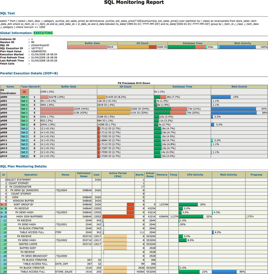
Figure 6-1. An HTML SQL Monitor Report
There are a couple limitations you should keep in mind regarding SQL Monitor Reports. Although SQL statement monitoring happens by default, as already mentioned, there are limits to how much monitoring data remain available. The hidden parameter _sqlmon_max_plan controls the size of the memory area dedicated to holding SQL monitoring information. By default, this parameter value is set to 20 times the number of CPUs. Therefore, if there are many different SQL statements being executed in your environment, it is entirely possible that the SQL statement monitoring data you are looking for may have already been pushed out because of newer SQL monitoring data needing space. Of course, you can increase this value if you want to attempt to keep monitoring data available for longer periods of time. But, as with changing any hidden parameter, you should do so with extreme caution and not without input from Oracle Support.
The second parameter that may cause you to not be able to produce a SQL Monitor Report for a given SQL statement is _sqlmon_max_planlines. This parameter defaults to 300 and limits the number of plan lines beyond which a statement is not monitored. In this case, if you have an extremely long execution plan of more than 300 lines, even if it is hinted with the MONITOR hint or if it runs long enough to be monitored normally automatically, it is not. As soon as the number of lines in the plan exceeds the 300 limit, monitoring is disabled.
You can use either a SQL Monitor Report or dbms_xplan.display_cursor output, as you prefer. I’ve started using SQL Monitor Reports more regularly because they require a bit less overhead to produce (because the STATISTICS_LEVEL parameter doesn’t need to be set to ALL to capture the statistics). Also, if you happen to be working on an Exadata platform, the SQL Monitor Report displays a column to include offload percentage, which tells you when full table scan operations use Exadata smart scan technology, and is a key indicator of performance on Exadata machines. This information isn’t present when using dbms_xplan.
Using Plan Information for Solving Problems
Now that you know how to access the various bits of information, what do you do with them? The plan information, particularly the plan statistics, helps you confirm how the plan is performing. You can use the information to determine whether there are any trouble spots, so you can then adjust the way the SQL is written, add or modify indexes, or even use the data to support a need to update statistics or adjust instance parameter settings.
Determining Index Deficiencies
If, for example, there is a missing or suboptimal index, you can see this in the plan. The next few listings walk through two examples: one shows how to determine whether an index is suboptimal (Listings 6-15 and 6-16) and the other shows how to determine an index is missing (Listing 6-17).
In each of these examples, there are two keys to look for. I made these example queries short and simple to keep the output easy to view, but regardless of how complex the plan, the way to spot a missing or suboptimal index is to look for (1) a TABLE ACCESS FULL operation with a filter predicate that shows a small A-Rows value (in other words, small in comparison with the total rows in the table) and (2) an index scan operation with a large A-Rows value compared with the parent TABLE ACCESS BY INDEX ROWID A-Rows value.
Listing 6-15. Using Plan Information to Determine Suboptimal Indexes
SQL> -- Example 1: sub-optimal index
SQL>
SQL> select /* KM1 */ job_id, department_id, last_name
  2  from employees
  3  where job_id = 'SA_REP'
  4  and department_id is null ;

JOB_ID       DEPARTMENT_ID LAST_NAME
---------- --------------- -------------------------
SA_REP     .               Grant

SQL> @pln KM1

PLAN_TABLE_OUTPUT
-----------------------------------------------------------------------------------
SQL_ID  0g7fpbvvbgvd2, child number 0
-------------------------------------
select /* KM1 */ job_id, department_id, last_name from hr.employees
where job_id = 'SA_REP' and department_id is null

Plan hash value: 2096651594

-------------------------------------------------------------------------
| Id  | Operation              | Name       | E-Rows | A-Rows | Buffers |
-------------------------------------------------------------------------
|   0 | SELECT STATEMENT       |            |        |      1 |       4 |
|*  1 |  TABLE ACCESS BY INDEX | EMPLOYEES  |      1 |      1 |       4 |
|     |      ROWID BATCHED     |            |        |        |         |
|*  2 |   INDEX RANGE SCAN     | EMP_JOB_IX |      6 |     30 |       2 |
-------------------------------------------------------------------------

Predicate Information (identified by operation id):
---------------------------------------------------

   1 - filter("DEPARTMENT_ID" IS NULL)
   2 - access("JOB_ID"='SA_REP')
So, how do we know the EMP_JOB_IX index is suboptimal? In Listing 6-15, notice the A-Rows statistic for each operation. The INDEX RANGE SCAN uses the job_id predicate to return 30 row IDs from the index leaf blocks that match ’SA_REP’. The parent step, TABLE ACCESS BY INDEX ROWID, retrieves rows by accessing the blocks as specified in the 30 row IDs it received from the child INDEX RANGE SCAN operation. When these 30 rows are retrieved, then the next condition for department_id is null must be checked. In the end, after all 30 rows (requiring four buffer accesses, as shown in the Buffers column) have been checked, only one row is actually a match to be returned in the query result set. This means that 97 percent of the rows that were accessed weren’t needed. From a performance perspective, this isn’t very effective. In this example, because the table is small (only 107 rows in five blocks), the problem this could cause isn’t really noticeable in terms of response time. But, why incur all that unnecessary work? That’s where creating a better index comes in. If we simply include both columns in the index definition, the index returns only one row ID, and the parent step does not have to access any data blocks that it has to throw away. Listing 6-16 shows how adding the additional column to the index decreases the total amount of rows accessed.
Listing 6-16. Adding a Column to an Index to Improve a Suboptimal Index
SQL> create index emp_job_dept_ix on employees (department_id, job_id) compute statistics ;
SQL>
SQL> select /* KM2 */ job_id, department_id, last_name
  2  from employees
  3  where job_id = 'SA_REP'
  4  and department_id is null ;

JOB_ID       DEPARTMENT_ID LAST_NAME
---------- --------------- -------------------------
SA_REP     .               Grant

SQL> @pln KM2

PLAN_TABLE_OUTPUT
-------------------------------------------------------------------------------
SQL_ID  a65qqjrawsbfx, child number 0
-------------------------------------
select /* KM2 */ job_id, department_id, last_name from hr.employees
where job_id = 'SA_REP' and department_id is null

Plan hash value: 1551967251

------------------------------------------------------------------------------
| Id  | Operation              | Name            | E-Rows | A-Rows | Buffers |
------------------------------------------------------------------------------
|   0 | SELECT STATEMENT       |                 |        |      1 |       2 |
|   1 |  TABLE ACCESS BY INDEX | EMPLOYEES       |      1 |      1 |       2 |
|     |      ROWID BATCHED     |                 |        |        |         |
|*  2 |   INDEX RANGE SCAN     | EMP_JOB_DEPT_IX |      1 |      1 |       1 |
------------------------------------------------------------------------------

Predicate Information (identified by operation id):
---------------------------------------------------

   2 - access("DEPARTMENT_ID" IS NULL AND "JOB_ID"='SA_REP')
       filter("JOB_ID"='SA_REP')
As you can see, by simply adding the department_id column to the index, the amount of work required to retrieve the query result set is minimized. The number of rowids passed from the child INDEX RANGE SCAN to the parent TABLE ACCESS BY INDEX ROWID step drops from 30 to just one, and the total buffer accesses is cut in half from four to two.
What about when no useful index exists? Again, this is a concern for performance. It may even be more of a concern than having a suboptimal index, because without any useful index at all, the only option the optimizer has is to use a full table scan. As the size of data increases, the responses are likely to keep increasing. So, you may “accidentally” miss creating an index in development when you are dealing with small amounts of data, but when data volumes increase in production, you’ll likely figure out you need an index pretty quick! Listing 6-17 demonstrates how to identify a missing index.
Listing 6-17. Using Plan Information to Determine Missing Indexes
SQL> -- Example 2: missing index
SQL>
SQL> select /* KM3 */ last_name, phone_number
  2  from employees
  3  where phone_number = '650.507.9822';

LAST_NAME                 PHONE_NUMBER
------------------------- --------------------
Feeney                    650.507.9822
SQL>
SQL> @pln KM3

PLAN_TABLE_OUTPUT
-------------------------------------------------------------------
SQL_ID  26ry1z7z20cat, child number 0
-------------------------------------
select /* KM3 */ last_name, phone_number from hr.employees where
phone_number = '650.507.9822'

Plan hash value: 1445457117

-------------------------------------------------------------------
| Id  | Operation         | Name      | E-Rows | A-Rows | Buffers |
-------------------------------------------------------------------
|   0 | SELECT STATEMENT  |           |        |      1 |       7 |
|*  1 |  TABLE ACCESS FULL| EMPLOYEES |      1 |      1 |       7 |
-------------------------------------------------------------------

Predicate Information (identified by operation id):
---------------------------------------------------

   1 - filter("PHONE_NUMBER"='650.507.9822')

SQL> column column_name format a22 heading 'Column Name'
SQL> column index_name heading 'Index Name'
SQL> column column_position format 999999999 heading 'Pos#'
SQL> column descend format a5 heading 'Order'
SQL> column column_expression format a40 heading 'Expression'
SQL>
SQL> break on index_name skip 1
SQL>
SQL> -- Check current indexes
SQL>
SQL> select  lower(b.index_name) index_name, b.column_position,
  2             b.descend, lower(b.column_name) column_name
  3  from       all_ind_columns b
  4  where      b.table_owner = 'HR'
  5  and        b.table_name = 'EMPLOYEES'
  6  order by b.index_name, b.column_position, b.column_name
  7  /

Index Name                           Pos# Order Column Name
------------------------------ ---------- ----- ------------------
emp_department_ix                       1 ASC   department_id

emp_email_uk                            1 ASC   email

emp_emp_id_pk                           1 ASC   employee_id

emp_job_dept_ix                         1 ASC   department_id
                                        2 ASC   job_id

emp_job_ix                              1 ASC   job_id

emp_manager_ix                          1 ASC   manager_id

emp_name_ix                             1 ASC   last_name
                                        2 ASC   first_name
In this example, the access operation chosen was a full table scan. By querying the ALL_IND_COLUMNS view, we can verify which indexes exist and on which columns. In this case, there is no index on the phone_number column, so the optimizer has no other choice than to use a full table scan and then filter the rows to locate any with a matching number. What is a bit difficult to tell just by looking is how much extra work it is to do the full scan and filter. In this case, the EMPLOYEES table has 107 rows, but the estimated number of rows only reflects how many rows are to be returned, not how many have to be accessed to check the filter condition. Because the query returned only one matching row for the phone number specified, this means 106 (virtually all) rows were rejected. Again, why incur all this work if having an index allows just the data you need to be accessed directly? Listing 6-18 shows what happens when the index is available.
Listing 6-18. Creating a New Index to Improve Performance
SQL> -- Create new index on phone_number
SQL>
SQL> create index hr.emp_phone_ix on hr.employees (phone_number) compute statistics ;
SQL>
SQL> select /* KM4 */ last_name, phone_number
  2  from employees
  3  where phone_number = '650.507.9822';

LAST_NAME                 PHONE_NUMBER
------------------------- --------------------
Feeney                    650.507.9822

SQL> @pln KM4

PLAN_TABLE_OUTPUT
----------------------------------------------------------------------------
SQL_ID  cs0bvb2zrsp66, child number 0
-------------------------------------
select /* KM4 */ last_name, phone_number from hr.employees where
phone_number = '650.507.9822'

Plan hash value: 2867517494

----------------------------------------------------------------------------
| Id  | Operation               | Name         | E-Rows | A-Rows | Buffers |
----------------------------------------------------------------------------
|   0 | SELECT STATEMENT        |              |        |      1 |       3 |
|   1 |  TABLE ACCESS BY INDEX  | EMPLOYEES    |      1 |      1 |       3 |
|     |     ROWID BATCHED       |              |        |        |         |
|*  2 |   INDEX RANGE SCAN      | EMP_PHONE_IX |      1 |      1 |       2 |
----------------------------------------------------------------------------

Predicate Information (identified by operation id):
---------------------------------------------------

   2 - access("PHONE_NUMBER"='650.507.9822')
With the index in place, the optimizer chooses it to access the rows needed to satisfy the query. Now, instead of having to check all 107 rows in the table, only the one row that matches the requested phone number is accessed via the index. The number of blocks accessed was cut by more than half from seven to three. Imagine if this table was larger!
Index Deficiencies Wrap-up
In both cases (either finding a missing index or determining the need for a new index), the main thing to watch out for is excess throwaway. The more blocks that have to be accessed to check filter conditions on rows that are ultimately not included in the result set, the poorer the performance becomes. You may not even notice it if data volume is low in the beginning, but the larger the tables become, the more effect accessing unneeded blocks has on response time.
Another way plan information can help you is by making it easy to spot when statistics might be out of date. Listing 6-19 shows an example of how plan information can point out stale statistics.
Listing 6-19. Using Plan Information to Determine When Statistics May Be out of Date
SQL> -- Check current column statistics (collected at 100%)
SQL>
SQL> select column_name, num_distinct, density
  2  from user_tab_cols
  3  where table_name = 'MY_OBJECTS' ;

Column Name            NUM_DISTINCT         DENSITY
------------------- --------------- ---------------
OWNER                            29 .03448275862069
OBJECT_NAME                   44245 .00002260142389
SUBOBJECT_NAME                  161 .00621118012422
OBJECT_ID                     72588 .00001377638177
DATA_OBJECT_ID                 7748 .00012906556531
OBJECT_TYPE                      44 .02272727272727
CREATED                        1418 .00070521861777
LAST_DDL_TIME                  1480 .00067567567568
TIMESTAMP                      1552 .00064432989691
STATUS                            1               1
TEMPORARY                         2              .5
GENERATED                         2              .5
SECONDARY                         2              .5
NAMESPACE                        21 .04761904761905
EDITION_NAME                      0               0

SQL> -- Execute query for object_type = 'TABLE'
SQL>
SQL> select /* KM7 */ object_id, object_name
  2  from my_objects
  3* where object_type = 'TABLE';
...
365056 rows selected.

SQL> @pln KM7

PLAN_TABLE_OUTPUT
---------------------------------------------------------------------------------
SQL_ID  7xphu2p2m9hdr, child number 0
-------------------------------------
select /* KM7 */ object_id, object_name from my_objects where
object_type = 'TABLE'

Plan hash value: 2785906523

------------------------------------------------------------------------------
| Id  | Operation               | Name           | E-Rows | A-Rows | Buffers |
------------------------------------------------------------------------------
|   0 | SELECT STATEMENT        |                |        |   365K |   55697 |
|   1 |  TABLE ACCESS BY INDEX  | MY_OBJECTS     |   1650 |   365K |   55697 |
|     |     ROWID BATCHED       |                |        |        |         |
|*  2 |   INDEX RANGE SCAN      | OBJECT_TYPE_IX |   1650 |   365K |   26588 |
------------------------------------------------------------------------------

Predicate Information (identified by operation id):
---------------------------------------------------

   2 - access("OBJECT_TYPE"='TABLE')
In this example, the optimizer computed that only 1650 rows would be returned by the query for OBJECT_TYPE = 'TABLE' when, in reality, the query returned more than 365,000 rows. Because I built the data for this table, I can tell you that this was because the statistics had been gathered prior to the addition of a few hundred thousand rows. When the plan was chosen, the optimizer didn’t have the updated information and it selected a plan using an index scan on the object_type index based on the old statistics. However, in reality, there were more than 474,000 total rows in the table and more than 365,000 of them matched the filter criteria. So, how do we correct the problem? Listing 6-20 shows one way you can identify the difference between the actual number of rows and the statistics value.
Listing 6-20. Identifying Difference Between Actual Rows and Statistics Rows Value
SQL> -- Compare statistic to actual
SQL>
SQL> select num_rows
  2  from dba_tables
  3  where table_name = 'MY_OBJECTS';

       NUM_ROWS
---------------
          72588

1 row selected.

SQL> select count(*)
  2  from my_objects ;

       COUNT(*)
---------------
         434792

1 row selected.

SQL> -- Update statistics
SQL>
SQL> exec dbms_stats.gather_table_stats(user,'MY_OBJECTS',estimate_percent=>100, cascade=>true,method_opt=>'FOR ALL COLUMNS SIZE 1'),

PL/SQL procedure successfully completed.
SQL> select /* KM8 */ object_id, object_name
  2  from my_objects
  3* where object_type = 'TABLE';
...
365056 rows selected.

SQL> @pln KM8

PLAN_TABLE_OUTPUT
----------------------------------------------------------------------------------------
SQL_ID  2qq7ram92zc85, child number 0
-------------------------------------
select /* KM8 */ object_id, object_name from my_objects where
object_type = 'TABLE'

Plan hash
value: 2785906523

------------------------------------------------------------------------------
| Id  | Operation               | Name           | E-Rows | A-Rows | Buffers |
------------------------------------------------------------------------------
|   0 | SELECT STATEMENT        |                |        |   365K |   54553 |
|   1 |  TABLE ACCESS BY INDEX  | MY_OBJECTS     |   9882 |   365K |   54553 |
|     |     ROWID BATCHED       |                |        |        |         |
|*  2 |   INDEX RANGE SCAN      | OBJECT_TYPE_IX |   9882 |   365K |   25444 |
------------------------------------------------------------------------------

Predicate Information (identified by operation id):
---------------------------------------------------

   2 - access("OBJECT_TYPE"='TABLE')
As this listing shows, when you determine that the actual number of rows in the table is significantly different than the number of rows captured by the statistics, a new collection is made and the query is executed again. This time, the estimate goes up to 9882 rows, but this is still an incorrect estimate compared with the actual rows returned. What happened? You collected fresh statistics and even used a 100 percent estimate, so everything should be correct, right? Well, the problem was that you didn’t collect histogram statistics, which tell the optimizer about the heavy skew in the distribution of values of the object_type column. You need to use a method_opt parameter that collects histograms. Actually, you need to use just the default method_opt parameter, which is FOR ALL COLUMNS SIZE AUTO. This value collects histograms on columns automatically. Listing 6-21 shows what happens after collecting histogram statistics and executing the query again.
Listing 6-21. Collecting Histogram Statistics
SQL> -- Collect histogram statistics
SQL>
SQL> exec dbms_stats.gather_table_stats(user,'MY_OBJECTS',estimate_percent=>100, cascade=>true,method_opt=>'FOR ALL COLUMNS SIZE AUTO'),

PL/SQL procedure successfully completed.

SQL> select /* KM9 */ object_id, object_name
  2  from my_objects
  3* where object_type = 'TABLE';
...
365056 rows selected.

SQL> @pln KM9

PLAN_TABLE_OUTPUT
-------------------------------------------------------------------------------------------
SQL_ID  dbvrtvutuyp6z, child number 0
-------------------------------------
select /* KM9 */ object_id, object_name from my_objects where
object_type = 'TABLE'

Plan hash value: 880823944

--------------------------------------------------------------------
| Id  | Operation         | Name       | E-Rows | A-Rows | Buffers |
--------------------------------------------------------------------
|   0 | SELECT STATEMENT  |            |        |    365K|   30000 |
|*  1 |  TABLE ACCESS FULL| MY_OBJECTS |    365K|    365K|   30000 |
--------------------------------------------------------------------

Predicate Information (identified by operation id):
---------------------------------------------------

   1 - filter("OBJECT_TYPE"='TABLE')
So, you did the collection again and this time used method_opt=>'FOR ALL COLUMNS SIZE AUTO'. This setting allows Oracle to collect a histogram properly on the object_type column. Now when you execute the query, the estimate is right on target and you get a full table scan plan instead. In this case, the full scan operation is the best choice because the query returns nearly 80 percent of all the rows in the table and a full scan accesses fewer blocks than an index scan plan would. We examine histograms and how statistics are used by the optimizer in a later chapter.
By the way, you could also check the STALE_STATS column value for the table in the DBA_TAB_STATISTICS view to determine whether statistics are out of date. This column shows a value of YES if there have been enough changes to the table to exceed a ten-percent threshold.
Summary
There is a wealth of information contained in plan output for every SQL statement. In this chapter, you saw how plan output can be obtained using EXPLAIN PLAN to get only estimated information, or how plan output can be obtained after executing the statement and extracting the plan information from the library cache using DBMS_XPLAN. In addition, plan information can be displayed using a SQL Monitor Report. At times, you may only be able to use EXPLAIN PLAN output, particularly if a query is very long-running and it is not easy or possible to wait to execute the query and get its actual execution data. However, to have the best information possible from which to make decisions about indexing, query syntax changes, or the need to update statistics or parameter settings, the use of actual plan execution statistics is the way to go. And, by using the active SQL Monitoring Report, you can even see the plan data while the statement is still executing, so you don’t have to wait until it completes to determine where the most time and resources are being consumed.
I covered some of the ways you can use plan information to help diagnose and solve performance problems for a SQL statement. By carefully reviewing plan output, you can uncover suboptimal or missing indexes and determine whether statistics are stale and need to be updated. Using the knowledge you’ve gained about the various plan operations for accessing and joining data, and understanding how to read and use plan information effectively, you are equipped not only to solve problems quickly and efficiently when they arise, but also to verify the characteristics and performance footprint of any SQL statement so that you can write well-behaved SQL from the start.