
![]()
As you’ve worked through the chapters of this book, you may have written some code to test the examples. And because you chose this particular book instead of a “Welcome to SQL”–style book, it’s likely you have written quite a few SQL statements before you ever picked it up. As you’ve been reading this book, did some of the chapters remind you of your prior work? If so, how do you feel about the code you’ve written in the past?
If you’re like most developers, there were times when you probably thought, “Hey, considering how little I knew about this functionality back then, I did pretty well.” And there may have been a few times when you cringed a bit, realizing that something you were very proud of at the time wasn’t such a great approach after all. Don’t worry; we all have applications that we would write completely differently if we only knew then what we know now. Besides, it’s always easier to write better code with hindsight or as an armchair code jockey.
If the code you write today is better than the code you wrote yesterday, you’re continuing to evolve and learn, and that is commendable. Realizing our older work could have been done better is an inevitable part of the learning process. As long as we learn from our mistakes and do a little better with the next application or the next bit of code, we’re moving in the right direction.
It’s also true that we need to be able to measure the quality of our current code now, not five years from now when we’ve grown even wiser. We want to find the problems in our code before they affect our users. Most of us want to find all the errors or performance issues before anyone else even sees our work. However, although this kind of attitude may indicate an admirable work ethic, it’s not an advisable or even an achievable goal. What we can achieve is a clear definition of what a specific piece of code needs to accomplish and how we can prove the code meets the defined requirements. Code should have measurable indicators of success that can prove or disprove the fact that we met our goal.
So what are these measurable factors? Although the target measurement varies depending on the application, there are several basic requirements for all application code. First and foremost, the code needs to return accurate results and we need to know that the results will continue to be accurate throughout the system’s life cycle. If end users cannot count on the data returned by a database application, that’s a pretty serious failure.
Performance is another measurable attribute of our code. The target runtimes are highly dependent on the application in question. A database used by a home owner’s association to track who has paid their annual fees is not required to perform at the same level as a database containing the current stock quotes, but the methods used to compare execution plans and measure runtime can be the same. Code quality requires that we understand the application requirements, the function being performed, and the strengths and weaknesses of the specific system. Testing should focus on verifying functionality, pushing the weakest links to their breaking point, and recording all measurements along the way.
For the examples in this chapter, we work with the same OE sample schema that we used for the transaction processing examples in Chapter 14. We make more changes to our schema, adding new data and altering views and reports. We begin by defining the changes to be made and the tests to use to verify the success of those changes.
So here is the backstory: One of our suppliers, identified only as Supplier 103089 in the database, is changing its product numbers for the software we purchase from them to resell to our customers. The new identifiers are appended with a hyphen and a two-character value to identify the software package language. For example, the supplier’s product identifier for all English software packages ends in -EN. The supplier requires its product identifier to be referenced for ordering, software updates, and warranty support. The new product identifiers have an effective date of October 10, 2010. This change presents the following challenges:
- The OE schema includes the supplier’s identifier in the product_information table, but the supplier product identifier is not stored in the sample schema database at all. We must alter the OE schema to add this field and create a numeric value to serve as the current supplier product ID. These changes are a prerequisite to the changes instituted by our supplier.
- After we have added an initial supplier product identifier for all the products we sell, we need to determine how we will add the modified product identifiers for this one supplier. We also need to have a method of controlling the effective date of the new identifiers.
- The purchasing department uses an inventory report to determine which products are getting low on stock. This report needs to reflect the current supplier product identifier until October 10, 2010. After that date, the report should print the new supplier product identifier so purchasing agents can place and verify orders easily.
- The OE system will continue to use our internal product identifier when orders are received from our customers. Orders and invoices must show our product identifier and name, plus the supplier product identifier.
- We have inventory on hand that is packaged with the current supplier product identifier. We can continue to sell those products as is, but our customer invoices must show the actual supplier product ID found on the packaging. This means our inventory system must treat the items labeled with the new numbering scheme as a distinct product.
As we make these changes, there are several basic tests and quality issues to consider. The points that follow are not intended to be all inclusive, because every system has its own unique test requirements; however, there are some quality checks that can be applied to all systems. Let’s use the following as a starting point:
- All objects that were valid before our changes should be valid when our changes are complete. Views, functions, procedures, and packages can be invalidated by a table change, depending on how the code for those objects was written originally. We need to check for invalid schema objects both before and after we make our changes. Objects that are invalidated as an indirect result of our planned modifications should recompile successfully without further changes.
- All data changes and results output must be accurate. Verifying data can be one of the more tedious tasks when developing or altering a database application, and the more data in the system, the more tedious the work. It’s also the most critical test our code must pass. If the data are not accurate, it doesn’t matter if the other requirements have been met or how fast the code executes. If the data being stored or returned cannot be trusted, our code is wrong and we’ve failed this most basic requirement. The simplest approach is to break down data verification into manageable components, beginning by verifying the core dataset, and then expand the test gradually to the more unique use cases (the “edge cases”) until we are certain all data are correct.
- Query performance can be verified by comparing the before and after versions of the execution plan. If the execution plan indicates the process has to work harder after our modifications, we want to be sure that additional work is, in fact, required and is not the result of a mistake. Use of execution plans was addressed in detail in Chapter 6, so we can refer back to that chapter for more information on the topic plus tips on making the best use of the information found in the execution plan.
Later in this chapter, I discuss code instrumentation and the Instrumentation Library for Oracle (ILO). ILO uses Oracle’s dbms_application_info procedures. Although it is possible to use the dbms_application_info procedures on their own, ILO makes it very easy and straightforward to add instrumentation to our code. I added some additional functionality to the ILO package; the updates are available for download at Apress. After the code is instrumented, these additional modules make it possible to build test systems that record processing times as iterative changes are made to the code or system configuration. These performance data make it very clear when changes have had a positive impact on processing times and when another approach should be considered.
Testing Methods
There are as many different approaches to software testing as there are software development—and there have quite possibly been an equal number of battles fought over both topics. Although it may be slightly controversial in a database environment, I advocate an approach known as test-driven development (TDD). TDD originated in the realm of extreme programming, so we need to make some modifications to the process to make it effective for database development, but it offers some very genuine benefits for both new development and modification efforts.
In TDD, developers begin by creating simple, repeatable tests that fail in the existing system but succeed after the change is implemented correctly. This approach has the following benefits:
- To write the test that fails, you have to understand thoroughly the requirements and the current implementation before you even begin to write application code.
- Building the unit test script first ensures that you start by working through the logic of the necessary changes, thereby decreasing the odds that your code has bugs or needs a major rewrite.
- By creating small, reusable unit tests to verify the successful implementation of a change, you build a library of test scripts that can be used both to test the initial implementation of the change and to confirm that the feature is still operating as expected as other system changes are made.
- These small-unit test scripts can be combined to create larger integration testing scripts or can become part of an automated test harness to simplify repetitive testing.
- TDD assists in breaking changes or new development into smaller, logical units of work. The subsets may be easier to understand and explain to other developers, which can be especially important when project members are not colocated.
- When test design is delayed until after development, testing frequently ends up being shortchanged, with incomplete or poorly written tests as a result of schedule constraints. Including test development efforts in the code development phases results in higher quality tests that are more accurate.
As acknowledged earlier, TDD needs some adjustments in a database environment or we run the risk of building yet another black box database application that is bound to fail performance and scalability testing. Whenever you develop or modify an application that stores or retrieves information from a database, as you prepare those first unit tests, you must consider the data model or work with the individuals responsible for that task. In my (sometimes) humble opinion, the data model is the single most important indicator of a database application’s potential to perform. The schema design is crucial to the application’s ability to scale for more users, more data, or both. This does not mean that development cannot begin until there is a flawless entity–relationship model, but it does mean that the core data elements must be understood and the application tables well designed for at least those core elements. And if the database model is not fully developed, then build the application using code that does not result in extensive changes as the data model is refactored.
So exactly what am I suggesting? To put it bluntly, if your application schema continues to be developed progressively, use procedures and packages for your application code. This allows the database to be refactored as data elements are moved or added, without requiring major front-end code rewrites.
![]() Note This is far from being a complete explanation of TDD or database refactoring. I strongly recommend the book Refactoring Databases: Evolutionary Database Design by Scott W. Ambler and Pramodkumar J. Sadalage (Addison-Wesley 2006) for a look at database development using Agile methods.
Note This is far from being a complete explanation of TDD or database refactoring. I strongly recommend the book Refactoring Databases: Evolutionary Database Design by Scott W. Ambler and Pramodkumar J. Sadalage (Addison-Wesley 2006) for a look at database development using Agile methods.
But let’s get back to our application changes, shall we? In the case of the changing supplier product identifier, let’s begin by asking some questions. How will this new data element be used by our company and employees? How will this change impact our OE and inventory data? Will this change impact systems or processes beyond our OE system? At a minimum, our purchasing agents need the supplier’s current product identifier to place an order for new products. Depending on how well recognized the component is, the supplier’s product identifier could be used more widely than we might expect; a specific product or component may even be a selling point with our customers. A great example is CPUs. The make and the model of the processor in the laptop can be far more important than the brand name on the case. If this is true for the products we are reselling, the supplier’s product ID may be represented throughout multiple systems beyond the ordering system, so it is necessary to extend our evaluation to include additional systems and processes.
As noted in the previous section, our first goal is to write the unit tests we need to demonstrate that our application modifications are successful. However, because this is a database application, we need to determine where this data element belongs before we can even begin to write the first unit test. Although the Oracle–provided sample schemas are far from perfect, we cannot refactor the entire schema in this chapter, so there are many data design compromises in the examples. This can also be true in the real world; it is seldom possible to make all the corrections we know should be made, which is why correcting problems in the schema design can be a long, iterative process that requires very careful management.
![]() Note Remember, the focus of this chapter is testing methods. I keep the examples as short as possible to avoid detracting from the core message. This means the examples do not represent production-ready code, nor do the sample schemas represent production-ready data models.
Note Remember, the focus of this chapter is testing methods. I keep the examples as short as possible to avoid detracting from the core message. This means the examples do not represent production-ready code, nor do the sample schemas represent production-ready data models.
Considering the primary OE functions that make use of the supplier product identifier, let’s store the supplier product ID in the product_information table. This table contains other descriptive attributes about the product and it is already used in the output reports that now need to include the newest data element. These are not the sole considerations when deciding where and how to store data, but for our purposes in this chapter, they will do. In the real world, the amount of data to be stored and accessed, the data values to be read most frequently, and how often specific data values are to be updated should all be considered prior to making decisions about where the data belong.
After we’ve decided where to keep the data, we can begin preparing the necessary unit tests for our change. So, what are the unit tests that fail before we add the supplier’s product ID to our schema? Here’s a list of the unit tests I cover in this chapter:
- Include the supplier’s product ID on individual orders and invoices.
- Print the supplier’s product ID on the open order summary report.
- Print a purchasing report that shows the current supplier’s product ID.
If we use a TDD process throughout development, then there are likely to be several generic unit tests that are already written and may be appropriate to include in this round of tests. Typical verification tests may focus on the following tasks:
- Confirm that all objects are valid before and after changes are made.
- Confirm that an insert fails if required constraints are not met.
- Verify that default values are populated when new data records are added.
- Execute a new order transaction with and without products from this specific supplier.
If we are thorough in our initial evaluation and unit test development work, we will know which tests are expected to fail. Other operations, such as the new order transaction I covered in Chapter 14, we expect to succeed, because we did not note that any changes are required for a new order. Should the existing unit tests for creating a new order fail after our changes, this indicates we did not analyze the impact of this latest change as thoroughly as we should have.
Before we make any changes to the database objects,let’s confirm the state of the existing objects. Preferably, all objects must be valid before we start making changes. This is important because it ensures we are aware of any objects that were invalid prior to our changes, and it helps us to recognize when we are responsible for invalidating the objects. Listing 15-1 shows a query to check for invalid objects and the result of the query.
Listing 15-1. Checking for Invalid Objects before Altering Database Objects
SQL> select object_name, object_type, last_ddl_time, status
       from user_objects where status != 'VALID';

no rows selected
Listing 15-2 shows our three unit test scripts. Each of these scripts represents a report that must include the correct supplier product identifier as related to our internal product number. The first test creates a report for a single order, which is essentially the customer’s invoice. The second test is the purchasing report, which must print the correct supplier product identifier plus the inventory on hand. The third unit test is a complete listing of all open orders, and it is built using several views.
Listing 15-2. Unit Test Scripts
--- order_report.sql

set linesize 115
column order_id new_value v_order noprint
column order_date new_value v_o_date noprint
column line_no format 99
column order_total format 999,999,999.99

BREAK ON order_id SKIP 2 PAGE
BTITLE OFF

compute sum of line_item_total on order_id

ttitle left 'Order ID: ' v_order         -
       right 'Order Date: ' v_o_date     -
       skip 2

spool logs/order_report.txt

select h.order_id ORDER_ID, h.order_date, li.line_item_id LINE_NO,
       li.supplier_product_id SUPP_PROD_ID, li.product_name, li.unit_price,
       li.discount_price, li.quantity, li.line_item_total
  from order_detail_header h, order_detail_line_items li
 where h.order_id = li.order_id
   and h.order_id = ‘&Order_Number’
 order by h.order_id, line_item_id ;

spool off

--- purchasing_report.sql

break on supplier skip 1
column target_price format 999,999.99
set termout off

spool logs/purchasing_report.txt

select p.supplier_id SUPPLIER, p.supplier_product_id SUPP_PROD_ID,
       p.product_name PRODUCT_NAME, i.quantity_on_hand QTY_ON_HAND,
       (p.min_price * .5) TARGET_PRICE
  from product_information p, inventories i
 where p.product_id = i.product_id
   and p.product_status = 'orderable'
   and i.quantity_on_hand < 1000
 order by p.supplier_id, p.supplier_product_id ;

spool off

set termout on

--- order_reports_all.sql

set linesize 115
column order_id new_value v_order noprint
column order_date new_value v_o_date noprint
column line_no format 99
column order_total format 999,999,999.99

BREAK ON order_id SKIP 2 PAGE
BTITLE OFF

compute sum of line_item_total on order_id

ttitle left 'Order ID: ' v_order         -
       right 'Order Date: ' v_o_date     -
       skip 2

select h.order_id ORDER_ID, h.order_date,
       li.line_item_id line_no, li.product_name, li.supplier_product_id ITEM_NO,
       li.unit_price, li.discount_price, li.quantity, li.line_item_total
  from order_detail_header h, order_detail_line_item li
 where h.order_id = li.order_id
order by h.order_id, li.line_item_id ;
Listing 15-3 shows the execution of our unit test scripts and the resulting (expected) failures.
Listing 15-3. Initial Unit Test Results
SQL> @ order_report.sql
       li.supplier_product_id,
       *
ERROR at line 2:
ORA-00904: "LI"."SUPPLIER_PRODUCT_ID": invalid identifier

SQL> @purchasing_report.sql
 order by p.supplier_id, p.supplier_product_id
                         *
ERROR at line 6:
ORA-00904: "P"."SUPPLIER_PRODUCT_ID": invalid identifier

SQL> @order_report_all.sql
 li.line_item_id line_no, li.product_name, li.supplier_product_id ITEM_NO,
                                           *
ERROR at line 2:
ORA-00904: "LI"."SUPPLIER_PRODUCT_ID": invalid identifier
Unit tests are typically created for and executed from the application interface, but it’s extremely helpful to create database-only unit tests as well. Having a set of scripts that we can run independently of the application code outside of the database allows us to check database functionality before we hand new code over to the test team. And if the front-end application tests result in unexpected errors, we already have information about a successful database-level execution, which helps both teams troubleshoot problems more efficiently.
Regression Tests
The goal of regression testing is to confirm that all prior functionality continues to work as expected. We must be certain that we do not reintroduce old issues (bugs) into our code as we implement new functionality. Regression tests are most likely to fail when there has not been adequate source code control, so someone inadvertently uses an obsolete piece of code as a starting point.
If unit tests are written for the existing functionality as the first step when the functionality is developed, those unit tests become the regression tests to confirm that each component of the system is still working as expected. In our case, the tests used to verify the order transaction process can be used to verify that orders are still processed as expected. Although I’m cheating a bit, I skip the reexecution of the OE transactions because I spent many pages on this topic in Chapter 14.
As a prerequisite to executing our examples, we need to make several changes to our schema to support storing a supplier product number at all. Let’s add a new varchar2 column in the product_information table to store the supplier_product_id field for each item we sell. We then populate the new column with a value to represent the current supplier product IDs for all the products we sell, and we use the dbms_random package to generate these numbers. When these data exist, our basic unit tests referencing the supplier product identifier should succeed.
However, to support the concept of effective product IDs, we must add new records to the product_information table using our supplier’s new identification values—a new internal product number with the same product description and pricing. Although we could update the existing records, this violates the requirement to reflect accurately the supplier’s product identifier shown on the product packaging in our warehouse. It also results in changing historical data, because we’ve already sold copies of this software to other customers. Although the software in the package is unchanged, the fact that our supplier has relabeled it essentially creates a brand new product, which is why we need these new product records. Let’s enter the new records with a product status of “planned,” because the effective date is in the future. On October 10, 2010, the new parts will be marked as “orderable” and the current parts become “obsolete.”
To manage the effective dates for the changing internal product identifiers, let’s create a new table: product_id_effectivity. Let’s also create a product_id sequence to generate our new internal identifiers, making certain that our sequence begins at a higher value that any of our existing product records. Although I don’t cover it in this chapter, this table could be used by a scheduled process that updates the product_status field in the product_information table to reflect whether a product is planned, orderable, or obsolete. It is the change in product status that triggers which supplier’s product ID is shown on the purchasing report, so purchasing agents can reference the correct number when placing new orders. Listing 15-4 shows the schema changes as they are processed.
Listing 15-4. Schema Changes and New Product Data
SQL> alter table product_information add supplier_product_id varchar2(15);

Table altered.

SQL> update product_information
        set supplier_product_id = round(dbms_random.value(100000, 80984),0) ;

288 rows updated.

SQL> commit;

Commit complete.

SQL> create sequence product_id start with 3525 ;

Sequence created.

SQL> create table product_id_effectivity (
       product_id           number,
       new_product_id       number,
       supplier_product_id  varchar(15),
       effective_date       date) ;

Table created.

SQL> insert into product_id_effectivity
     (select product_id, product_id.nextval,
             round(dbms_random.value(100000, 80984),0)||'-'||
            substr(product_name, instr(product_name,'/',-1,1)+1), '10-oct-10'
        from product_information, dual
       where supplier_id = 103089
         and product_name like '%/%') ;
9 rows created.
SQL> select * from product_id_effectivity ;
PRODUCT_ID NEW_PRODUCT_ID SUPPLIER_PRODUC EFFECTIVE_DATE
---------- -------------- --------------- -------------------
      3170           3525 93206-SP        0010-10-10 00:00:00
      3171           3526 84306-EN        0010-10-10 00:00:00
      3176           3527 89127-EN        0010-10-10 00:00:00
      3177           3528 81889-FR        0010-10-10 00:00:00
      3245           3529 96987-FR        0010-10-10 00:00:00
      3246           3530 96831-SP        0010-10-10 00:00:00
      3247           3531 85011-DE        0010-10-10 00:00:00
      3248           3532 88474-DE        0010-10-10 00:00:00
      3253           3533 82876-EN        0010-10-10 00:00:00
9 rows selected.
SQL> commit ;
Commit complete.
SQL>  insert into product_information (
             product_id, product_name, product_description, category_id,
             weight_class, supplier_id, product_status, list_price, min_price,
             catalog_url, supplier_product_id)
         (select e.new_product_id,
                 p.product_name,
                 p.product_description,
                 p.category_id,
                 p.weight_class,
                 p.supplier_id,
                  'planned',
                 p.list_price,
                 p.min_price,
                 p.catalog_url,
                 e.supplier_product_id
            from product_information p, product_id_effectivity e
           where p.product_id = e.product_id
             and p.supplier_id = 103089) ;
9 rows created.

SQL> select product_id, product_name, product_status, supplier_product_id
       from product_information
      where supplier_id = 103089
      order by product_id ;

PRODUCT_ID PRODUCT_NAME                      PRODUCT_STATUS       SUPPLIER_PRODUC
---------- --------------------------------- -------------------- ---------------
      3150 Card Holder - 25                  orderable            3150
      3170 Smart Suite - V/SP                orderable            3170
      3171 Smart Suite - S3.3/EN             orderable            3171
      3175 Project Management - S4.0         orderable            3175
      3176 Smart Suite - V/EN                orderable            3176
      3177 Smart Suite - V/FR                orderable            3177
      3245 Smart Suite - S4.0/FR             orderable            3245
      3246 Smart Suite - S4.0/SP             orderable            3246
      3247 Smart Suite - V/DE                orderable            3247
      3248 Smart Suite - S4.0/DE             orderable            3248
      3253 Smart Suite - S4.0/EN             orderable            3253
      3525 Smart Suite - V/SP                planned              93206-SP
      3526 Smart Suite - S3.3/EN             planned              84306-EN
      3527 Smart Suite - V/EN                planned              89127-EN
      3528 Smart Suite - V/FR                planned              81889-FR
      3529 Smart Suite - S4.0/FR             planned              96987-FR
      3530 Smart Suite - S4.0/SP             planned              96831-SP
      3531 Smart Suite - V/DE                planned              85011-DE
      3532 Smart Suite - S4.0/DE             planned              88474-DE
      3533 Smart Suite - S4.0/EN             planned              82876-EN

20 rows selected.
After we’ve completed the necessary schema updates, our next step is to check for invalid objects again. All objects were valid when we ran our initial check, but now we altered a table that is likely to be referenced by several other code objects in our schema. If those objects are coded properly, we can recompile them as is and they become valid again. If the code is sloppy (perhaps we used a select * from product_information clause to populate an object that does not have the new field), then the recompile fails and we need to plan for more application modifications. The unit test to look for invalid objects, plus the two recompiles that are required after our changes, are shown in Listing 15-5.
Listing 15-5. Invalid Objects Unit Test and Object Recompile
SQL> select object_name, object_type, last_ddl_time, status
       from user_objects
      where status != 'VALID';

OBJECT_NAME                         OBJECT_TYPE         LAST_DDL_ STATUS
----------------------------------- ------------------- --------- -------
GET_ORDER_TOTAL                     PROCEDURE           04-jul-10 INVALID
GET_LISTPRICE                       FUNCTION            04-jul-10 INVALID

SQL> alter function GET_LISTPRICE compile ;

Function altered.

SQL> alter procedure GET_ORDER_TOTAL compile ;

Procedure altered.

SQL> select object_name, object_type, last_ddl_time, status
       from user_objects
      where status != 'VALID';

no rows selected
Repeating the Unit Tests
After we’ve confirmed that our planned schema changes have implemented successfully and all objects are valid, it’s time to repeat the remaining unit tests. This time, each of the tests should execute and we should be able to verify that the supplier’s product ID is represented accurately in the data results. Results from the second execution of the unit test are shown in Listing 15-6. To minimize the number of trees required to print this book, output from the reports is abbreviated.
Listing 15-6. Second Execution of Unit Tests
SQL> @order_report

Order ID:5041 Order Date: 13 Jul 2010

 NO SUP_PROD_ID PRODUCT_NAME              UNIT_PRICE DISC_PRICE  QTY ITEM_TOTAL
--- ----------- ------------------------- ---------- ---------- ---- ----------
  1 98811       Smart Suite - S4.0/DE         222.00     199.80    5     999.00

SQL> @purchasing_report

  SUPPLIER S_PRODUCT    PRODUCT_NAME            QTY_ON_HAND TARGET_PRICE
---------- ------------ ----------------------- ----------- ------------
    103086 96102        IC Browser Doc - S              623        50.00

    103088 83069        OSI 1-4/IL                       76        36.00

    103089 86151        Smart Suite - S4.0/EN           784        94.00
           89514        Smart Suite - V/DE              290        48.00
           92539        Smart Suite - V/EN              414        51.50
           93275        Smart Suite - V/FR              637        51.00
           95024        Smart Suite - S4.0/SP           271        96.50
           95857        Smart Suite - V/SP              621        66.00
           98796        Smart Suite - S3.3/EN           689        60.00
           98811        Smart Suite - S4.0/DE           114        96.50
           99603        Smart Suite - S4.0/FR           847        97.50
.......

SQL> @order_report_all.sql

Order ID: 2354                                                Order Date: 14 Jul 2002
ID PRODUCT_NAME               ITEM_NO UNIT_PRICE DISCOUNT_PRICE   QTY LINE_ITEM_TOTAL
--- ------------------------ -------- ---------- -------------- ----- ---------------
  1 KB 101/EN                   94979      48.00          45.00    61        2,745.00
  1 KB 101/EN                   98993      48.00          45.00    61        2,745.00
  1 KB 101/EN                   85501      48.00          45.00    61        2,745.00
.......

Order ID: 5016                                                Order Date: 06 Jul 2010
 ID PRODUCT_NAME              ITEM_NO UNIT_PRICE DISCOUNT_PRICE   QTY LINE_ITEM_TOTAL
--- ------------------------ -------- ---------- -------------- ----- ---------------
  1 Inkvisible Pens             86030       6.00           5.40  1000        5,400.00

Order ID: 5017                                                Order Date: 06 Jul 2010
 ID PRODUCT_NAME              ITEM_NO UNIT_PRICE DISCOUNT_PRICE   QTY LINE_ITEM_TOTAL
--- ------------------------ -------- ---------- -------------- ----- ---------------
  1 Compact 400/DQ              87690     125.00         118.75    25        2,968.75

Order ID: 5041                                                Order Date: 13 Jul 2010
 ID PRODUCT_NAME              ITEM_NO UNIT_PRICE DISCOUNT_PRICE   QTY LINE_ITEM_TOTAL
--- ------------------------ -------- ---------- -------------- ----- ---------------
  1 Smart Suite - S4.0/DE       98811     222.00         199.80     5          999.00
Take note that in each case when the product name shows a product that will be affected by our supplier’s new identifiers, our reports still show the current supplier identifier. This is because these reports were prior to the October 10, 2010, effective date. What we have not yet addressed in our testing is a mechanism to set to “obsolete” products referencing the old supplier product identifiers and to make our new products referencing the new supplier product identifier “orderable.” After the effective date passes, we need the purchasing report in particular to reference the new IDs. Order data should continue to represent the item ordered and shipped, which is not necessarily determined by the effective date for the part number change. Instead, we want our sales team to sell the older product first, so we only begin to see the new product identifiers on orders and invoices after the existing inventory is depleted. This thought process should trigger the development of a few more unit tests, such as testing the process to alter product status after a product change effective date had passed, and confirming that the OE system does not make the new product identifiers available for purchase until the old stock has been depleted.
One of the best tools available for evaluating the impact of the changes you make to database objects and code is the execution plan. By recording the execution plan both before and after our changes, we have a detailed measurement of exactly how much work the database needs to complete to process requests for the data in the past, and how much work is required to process those same requests in the future. If the comparison of the before and after versions of the execution plan indicates that a significant amount of additional work is required, it may be necessary to reevaluate the code to determine whether it can be optimized. If the process is already as optimized as it can be, you can then use the information to explain, nicely, to the users that their report may take longer to run in the future because of the added functionality. When you express your findings in these terms, you will discover exactly how much the users value that new functionality, and it is up to them to decide whether the changes are important enough to move to production.
Comparing the execution plans can also make it very clear when there is something wrong with a query. If you find that a process is working much harder to get the data, but the new changes don’t justify the additional work, there is a strong possibility there is an error in the code somewhere.
For the next example, let’s review the execution plans of the complete order report from our unit testing. The execution plan recorded before we made any changes to the database is shown in Listing 15-7. The scripts to gather the execution plans are based on the approach demonstrated in Chapter 6.
Listing 15-7. Order Report Execution Plan (Before)
alter session set statistics_level = 'ALL';

set linesize 105
column order_id new_value v_order noprint
column order_date new_value v_o_date noprint
column ID format 99
column order_total format 999,999,999.99

BREAK ON order_id SKIP 2 PAGE
BTITLE OFF

compute sum of line_item_total on order_id

ttitle left 'Order ID: ' v_order          -
       right 'Order Date: ' v_o_date      -
       skip 2

spool logs/order_report_all_pre.txt
select /* OrdersPreChange */ h.order_id ORDER_ID, order_date,
       li.line_item_id ID, li.product_name, li.product_id ITEM_NO,
       li.unit_price, li.discount_price, li.quantity, li.line_item_total
  from order_detail_header h, order_detail_line_items li
 where h.order_id = li.order_id
 order by h.order_id, li.line_item_id ;

spool off

set lines 150
spool logs/OrdersPreChange.txt

@pln.sql OrdersPreChange

PLAN_TABLE_OUTPUT
------------------------------------------------------------------------------------------
SQL_ID  ayucrh1mf6v4s, child number 0
-------------------------------------
select /* OrdersPreChange */ h.order_id ORDER_ID, order_date,
li.line_item_id ID, li.product_name, li.product_id ITEM_NO,
li.unit_price, li.discount_price, li.quantity, li.line_item_total
from order_detail_header h, order_detail_line_items li  where
h.order_id = li.order_id  order by h.order_id, li.line_item_id

Plan hash value: 3662678147

-------------------------------------------------------------------------------------------
| Id  |Operation                     |Name               |Starts |E-Rows |A-Rows |Buffers |
-------------------------------------------------------------------------------------------
|   0 |SELECT STATEMENT              |                   |     1 |       |   417 |     29 |
|   1 | SORT ORDER BY                |                   |     1 |   474 |   417 |     29 |
|*  2 |  HASH JOIN                   |                   |     1 |   474 |   417 |     29 |
|   3 |   TABLE ACCESS FULL          |PRODUCT_INFORMATION|     1 |   297 |   297 |     16 |
|   4 |   NESTED LOOPS               |                   |     1 |   474 |   417 |     13 |
|   5 |    MERGE JOIN                |                   |     1 |   474 |   417 |      9 |
|*  6 |     TABLE ACCESS BY INDEX ROW|ORDERS             |     1 |    79 |    79 |      2 |
|   7 |      INDEX FULL SCAN         |ORDER_PK           |     1 |   114 |   114 |      1 |
|*  8 |     SORT JOIN                |                   |    79 |   678 |   417 |      7 |
|   9 |      TABLE ACCESS FULL       |ORDER_ITEMS        |     1 |   678 |   678 |      7 |
|* 10 |    INDEX UNIQUE SCAN         |ORDER_STATUS_PK    |   417 |     1 |   417 |      4 |
-------------------------------------------------------------------------------------------

Predicate Information (identified by operation id):
---------------------------------------------------

   2 - access("OI"."PRODUCT_ID"="PI"."PRODUCT_ID")
   6 - filter("O"."SALES_REP_ID" IS NOT NULL)
   8 - access("O"."ORDER_ID"="OI"."ORDER_ID")
       filter("O"."ORDER_ID"="OI"."ORDER_ID")
  10 - access("O"."ORDER_STATUS"="OS"."ORDER_STATUS")

35 rows selected.
The order report is generated by joining two views: the order header information and the order line item details. Let’s assume the report is currently running fast enough to meet user requirements and that there are no indicators that the quantity of data in the underlying tables is expected to increase dramatically in the future. The report is deemed as meeting requirements, and the execution plan is saved for future reference.
This order report was executed as one of our first unit tests to verify that our unit tests work as expected. After we make the required database changes, we execute the order report again and confirm that it completes. The report also seems to complete in about the same amount of time as it did in the past, but let’s take a look at the latest execution plan to determine how the report is really performing. The postchange execution plan is shown in Listing 15-8.
Listing 15-8. Order Report Execution Plan (After)
alter session set statistics_level = 'ALL';

set linesize 115
column order_id new_value v_order noprint
column order_date new_value v_o_date noprint
column ID format 99
column order_total format 999,999,999.99

BREAK ON order_id SKIP 2 PAGE
BTITLE OFF

compute sum of line_item_total on order_id

ttitle left 'Order ID: ' v_order          -
       right 'Order Date: ' v_o_date      -
       skip 2

spool logs/order_report_all_fail.txt

select /* OrdersChangeFail */ h.order_id ORDER_ID, order_date,
       li.line_item_id ID, li.product_name, p.supplier_product_id ITEM_NO,
       li.unit_price, li.discount_price, li.quantity, li.line_item_total
  from order_detail_header h, order_detail_line_items li,
       product_information p
 where h.order_id = li.order_id
   and li.product_id = p.product_id
 order by h.order_id, li.line_item_id ;

spool off

set lines 150
spool logs/OrdersChangeFail.log

@pln.sql OrdersChangeFail

PLAN_TABLE_OUTPUT
-------------------------------------------------------------------------------------------
SQL_ID  avhuxuj0d23kc, child number 0
-------------------------------------
select /* OrdersChangeFail */ h.order_id ORDER_ID, order_date,
li.line_item_id ID, li.product_name, p.supplier_product_id ITEM_NO,
   li.unit_price, li.discount_price, li.quantity, li.line_item_total
from order_detail_header h, order_detail_line_items li,
product_information p  where h.order_id = li.order_id    and
li.product_id = p.product_id  order by h.order_id, li.line_item_id

Plan hash value: 1984333101

-------------------------------------------------------------------------------------------
| Id  |Operation                     |Name               |Starts |E-Rows |A-Rows |Buffers |
-------------------------------------------------------------------------------------------
|   0 |SELECT STATEMENT              |                   |     1 |       |   417 |     45 |
|   1 | SORT ORDER BY                |                   |     1 |   474 |   417 |     45 |
|*  2 |  HASH JOIN                   |                   |     1 |   474 |   417 |     45 |
|   3 |   TABLE ACCESS FULL          |PRODUCT_INFORMATION|     1 |   297 |   297 |     16 |
|*  4 |   HASH JOIN                  |                   |     1 |   474 |   417 |     29 |
|   5 |    TABLE ACCESS FULL         |PRODUCT_INFORMATION|     1 |   297 |   297 |     16 |
|   6 |    NESTED LOOPS              |                   |     1 |   474 |   417 |     13 |
|   7 |     MERGE JOIN               |                   |     1 |   474 |   417 |      9 |
|*  8 |      TABLE ACCESS BY INDEX RO|ORDERS             |     1 |    79 |    79 |      2 |
|   9 |       INDEX FULL SCAN        |ORDER_PK           |     1 |   114 |   114 |      1 |
|* 10 |      SORT JOIN               |                   |    79 |   678 |   417 |      7 |
|  11 |       TABLE ACCESS FULL      |ORDER_ITEMS        |     1 |   678 |   678 |      7 |
|* 12 |     INDEX UNIQUE SCAN        |ORDER_STATUS_PK    |   417 |     1 |   417 |      4 |
-------------------------------------------------------------------------------------------

Predicate Information (identified by operation id):
---------------------------------------------------

   2 - access("PI"."PRODUCT_ID"="P"."PRODUCT_ID")
   4 - access("OI"."PRODUCT_ID"="PI"."PRODUCT_ID")
   8 - filter("O"."SALES_REP_ID" IS NOT NULL)
  10 - access("O"."ORDER_ID"="OI"."ORDER_ID")
       filter("O"."ORDER_ID"="OI"."ORDER_ID")
  12 - access("O"."ORDER_STATUS"="OS"."ORDER_STATUS")

39 rows selected.
Looking at this latest plan, the database is doing much more work after our changes, even though the report is not taking any appreciable amount of extra time to complete. There is no good reason for this to be so; we’ve only added one additional column to a table that was already the central component of the query. Furthermore, the table in question already required a full table scan, because most of the columns are needed for the report. But, the execution plan shows that our report is now doing two full table scans of the product_information table. Why?
In this case, I made a common error deliberately to illustrate how an execution plan can help find quality problems in changed code. Rather than simply add the new column to the existing order_detail_line_item view that is built on the product_information table, the product_information table has been joined to the order_detail_line_item view, resulting in a second full table scan of the central table.
This probably seems like a really foolish mistake to make, but it can be done easily. I’ve seen many developers add a new column to a query by adding a new join to a table or view that was already part of the existing report. This error has a clear and visible impact on an execution plan, especially if the query is complex (and it usually is when this type of error is made). Listing 15-9 shows the execution plan for the same query after the additional join is removed and the column is added to the existing order_detail_line_item view instead.
Listing 15-9. Order Report Execution Plan (Corrected)
alter session set statistics_level = 'ALL';

set linesize 115
column order_id new_value v_order noprint
column order_date new_value v_o_date noprint
column ID format 99
column order_total format 999,999,999.99

BREAK ON order_id SKIP 2 PAGE
BTITLE OFF

compute sum of line_item_total on order_id

ttitle left 'Order ID: ' v_order          -
       right 'Order Date: ' v_o_date      -
       skip 2

spool logs/order_report_all_corrected.txt

select /* OrdersCorrected */ h.order_id ORDER_ID, order_date,
       li.line_item_id ID, li.product_name, li.supplier_product_id ITEM_NO,
       li.unit_price, li.discount_price, li.quantity, li.line_item_total
  from order_detail_header h, order_detail_line_items li
 where h.order_id = li.order_id
 order by h.order_id, li.line_item_id ;

spool off

set lines 150
spool logs/OrdersCorrected_plan.txt

@pln.sql OrdersCorrected

PLAN_TABLE_OUTPUT
--------------------------------------------------------------------------------------------
SQL_ID  901nkw7f6fg4r, child number 0
-------------------------------------
select /* OrdersCorrected */ h.order_id ORDER_ID, order_date,
li.line_item_id ID, li.product_name, li.supplier_product_id ITEM_NO,
    li.unit_price, li.discount_price, li.quantity, li.line_item_total
from order_detail_header h, order_detail_line_items li  where
h.order_id = li.order_id  order by h.order_id, li.line_item_id

Plan hash value: 3662678147
-------------------------------------------------------------------------------------------
| Id  |Operation                     |Name               |Starts |E-Rows |A-Rows |Buffers |
-------------------------------------------------------------------------------------------
|   0 |SELECT STATEMENT              |                   |      1|       |   417 |     29 |
|   1 | SORT ORDER BY                |                   |      1|    474|   417 |     29 |
|*  2 |  HASH JOIN                   |                   |      1|    474|   417 |     29 |
|   3 |   TABLE ACCESS FULL          |PRODUCT_INFORMATION|      1|    297|   297 |     16 |
|   4 |   NESTED LOOPS               |                   |      1|    474|   417 |     13 |
|   5 |    MERGE JOIN                |                   |      1|    474|   417 |      9 |
|*  6 |     TABLE ACCESS BY INDEX ROW|ORDERS             |      1|     79|    79 |      2 |
|   7 |      INDEX FULL SCAN         |ORDER_PK           |      1|    114|   114 |      1 |
|*  8 |     SORT JOIN                |                   |     79|    678|   417 |      7 |
|   9 |      TABLE ACCESS FULL       |ORDER_ITEMS        |      1|    678|   678 |      7 |
|* 10 |    INDEX UNIQUE SCAN         |ORDER_STATUS_PK    |    417|      1|   417 |      4 |
-------------------------------------------------------------------------------------------

Predicate Information (identified by operation id):
---------------------------------------------------

   2 - access("OI"."PRODUCT_ID"="PI"."PRODUCT_ID")
   6 - filter("O"."SALES_REP_ID" IS NOT NULL)
   8 - access("O"."ORDER_ID"="OI"."ORDER_ID")
       filter("O"."ORDER_ID"="OI"."ORDER_ID")
  10 - access("O"."ORDER_STATUS"="OS"."ORDER_STATUS")

35 rows selected.
As you can see by this latest execution plan, our report now performs as expected, with no additional impact to performance or use of system resources.
One of my favorite Oracle features is instrumentation. The database itself is fully instrumented, which is why we can see exactly when the database is waiting and what it is waiting for. Without this instrumentation, a database is something like a black box, providing little information about where resources are spending, or not spending, their time.
Oracle also provides the dbms_application_info package, which we can use to instrument the code we write. This package allows us to label the actions and modules within the code so that we can identify more easily which processes in the application are active. We can also combine our instrumentation data with Oracle’s Active Session History (ASH), Active Workload Repository (AWR), and other performance management tools to gain further insight into our application’s performance while easily filtering out other unrelated processes.
The simplest method I know for adding instrumentation to application code is the ILO, which is available at http://sourceforge.net/projects/ilo/. ILO is open-source software written and supported by my friends at Method-R. Method-R also offers the option to purchase a license for ILO so that it can be used in commercial software products. I’ve been using ILO to instrument code for several years, and I’ve added functionality to the 2.3 version. The enhancements allow me to record the exact start and stop time of an instrumented process using the database’s internal time references. These data can then be used to calculate statistical indicators on process execution times, which helps to highlight potential performance issues before they become major problems. I’ve also added code to enable extended SQL tracing (10046 event) for a specific process by setting an on/off switch in a table. So, if I determine that I need trace data for a specific application process, I can set tracing to ON for that process by its instrumented process name and it is traced every time it executes until tracing is set to OFF again. The configuration module can also be used to set the elapsed time collection ON or OFF, but I usually prefer to leave elapsed time recording on and purge older data when they are no longer useful.
If you’d like to test the ILO instrumentation software as you go through the next few sections, start by downloading ILO 2.3 from SourceForge.net and install it per the instructions. You can then download the code to store elapsed time and set the trace and timing configuration from the Apress download site. Instructions to add the updates are included in the ZIP file.
Adding Instrumentation to Code
After you’ve installed the ILO schema, adding instrumentation to your application is done easily. There are several ways to accomplish this. Of course, you need to determine the best method and the appropriate configuration based on your environment and requirements, but here are a few general guidelines:
- Within your own session, you can turn timing and tracing on or off at any time. You can also instrument any of your SQL statements (1) by executing the ILO call to begin a task before you execute your SQL statement and (2) by executing the call to end the task after the statement. This approach is shown in Listing 15-10.
Listing 15-10. ILO Execution in a Single Session
SQL> exec ilo_timer.set_mark_all_tasks_interesting(TRUE,TRUE);

PL/SQL procedure successfully completed.

SQL> exec ilo_task.begin_task('Month-end','Purchasing'),

PL/SQL procedure successfully completed.

SQL> @purchasing_report

SQL> exec ilo_task.end_task;

PL/SQL procedure successfully completed.

   Selected from ILO_ELAPSED_TIME table:

   INSTANCE: TEST
   SPID: 21509
   ILO_MODULE: Month-end
   ILO_ACTION: Purchasing
   START_TIME: 22-SEP-13 06.08.19.000000 AM
   END_TIME: 22-SEP-13 06.09.06.072642 AM
   ELAPSED_TIME: 46.42
   ELAPSED_CPUTIME: .01
ERROR_NUM: 0 - You can encapsulate your code within a procedure and include the calls to ILO within the procedure itself. This has the added advantage of ensuring that every call to the procedure is instrumented and that the ILO action and module are labeled consistently. Consistent labeling is very important if you want to aggregate your timing data in a meaningful way or to track trends in performance. We look at the billing.credit_request procedure from Chapter 14 with added calls to ILO in Listing 15-11.
Listing 15-11. Incorporating ILO into a Procedure
create or replace procedure credit_request(p_customer_id      IN   NUMBER,
                                           p_amount           IN   NUMBER,
                                           p_authorization    OUT  NUMBER,
                                           p_status_code      OUT  NUMBER,
                                           p_status_message   OUT  VARCHAR2)
 IS

  /*************************************************************************
      status_code values
        status_code status_message
        =========== =======================================================
                  0  Success
             -20105  Customer ID must have a non-null value.
             -20110  Requested amount must have a non-null value.
             -20500  Credit Request Declined.
  *************************************************************************/
   v_authorization NUMBER;
BEGIN
  ilo_task.begin_task('New Order', 'Credit Request'),

  SAVEPOINT RequestCredit;

  IF ( (p_customer_id) IS NULL ) THEN
    RAISE_APPLICATION_ERROR(-20105, 'Customer ID must have a non-null value.', TRUE);
  END IF;

  IF ( (p_amount) IS NULL ) THEN
    RAISE_APPLICATION_ERROR(-20110, 'Requested amount must have a non-null value.', TRUE);
  END IF;

   v_authorization := round(dbms_random.value(p_customer_id, p_amount), 0);

  IF ( v_authorization between 324 and 342 ) THEN
    RAISE_APPLICATION_ERROR(-20500, 'Credit Request Declined.', TRUE);
  END IF;

  p_authorization:= v_authorization;
  p_status_code:= 0;
  p_status_message:= NULL;

  ilo_task.end_task;

EXCEPTION
  WHEN OTHERS THEN
    p_status_code:= SQLCODE;
    p_status_message:= SQLERRM;

    BEGIN
      ROLLBACK TO SAVEPOINT RequestCredit;
    EXCEPTION WHEN OTHERS THEN NULL;
    END;

    ilo_task.end_task(error_num => p_status_code);

END credit_request;
/

Execution Script:

set serveroutput on

DECLARE
  P_CUSTOMER_ID      NUMBER;
  P_AMOUNT           NUMBER;
  P_AUTHORIZATION    NUMBER;
  P_STATUS_CODE      NUMBER;
  P_STATUS_MESSAGE   VARCHAR2(200);

BEGIN
  P_CUSTOMER_ID := '&customer';
  P_AMOUNT := '&amount';

  billing.credit_request(
    P_CUSTOMER_ID => P_CUSTOMER_ID,
    P_AMOUNT => P_AMOUNT,
    P_AUTHORIZATION => P_AUTHORIZATION,
    P_STATUS_CODE => P_STATUS_CODE,
    P_STATUS_MESSAGE => P_STATUS_MESSAGE
  );
commit;

  DBMS_OUTPUT.PUT_LINE('P_CUSTOMER_ID = ' || P_CUSTOMER_ID);
  DBMS_OUTPUT.PUT_LINE('P_AMOUNT = ' || P_AMOUNT);
  DBMS_OUTPUT.PUT_LINE('P_AUTHORIZATION = ' || P_AUTHORIZATION);
  DBMS_OUTPUT.PUT_LINE('P_STATUS_CODE = ' || P_STATUS_CODE);
  DBMS_OUTPUT.PUT_LINE('P_STATUS_MESSAGE = ' || P_STATUS_MESSAGE);

END;
/

Execution:

SQL> @exec_CreditRequest
Enter value for customer: 237
Enter value for amount: 10000

P_CUSTOMER_ID = 237
P_AMOUNT = 10000
P_AUTHORIZATION = 8302
P_STATUS_CODE = 0
P_STATUS_MESSAGE =

PL/SQL procedure successfully completed.

SQL> @exec_CreditRequest
Enter value for customer: 334
Enter value for amount: 500

P_CUSTOMER_ID = 237
P_AMOUNT = 500
P_AUTHORIZATION =
P_STATUS_CODE = -20500
P_STATUS_MESSAGE = ORA-20500: Credit Request Declined.

PL/SQL procedure successfully completed.

   Selected from ILO_ELAPSED_TIME table:

   INSTANCE: TEST
   SPID: 3896
   ILO_MODULE: New Order
   ILO_ACTION: Request Credit
   START_TIME: 22-SEP-13 01.43.41.000000 AM
   END_TIME: 22-SEP-13 01.43.41.587155 AM
   ELAPSED_TIME: .01
   ELAPSED_CPUTIME: 0
ERROR_NUM: 0 - You can create an application-specific wrapper to call the ILO procedures. One benefit of using a wrapper is that you can make sure a failure in ILO does not result in a failure for the application process. Although you do want good performance data, you don’t want to prevent the application from running because ILO isn’t working. A simple wrapper is included with the ILO update download at Apress.
The level of granularity you decide to implement with your instrumentation depends on your goals. For some tasks, it is perfectly acceptable to include multiple processes in a single ILO module or action. For critical code, I recommend that you instrument the individual processes with their own action and module values, which gives more visibility into complex procedures. If you are supporting an application that is not instrumented and it seems like too big a task to go back and instrument all the existing code, consider adding the instrumentation just to the key processes.
Again, how you decide to implement depends on your needs. Instrumentation is exceptionally useful for testing code and configuration changes during development and performance testing. After the calls to ILO have been built into the code, you can turn timing/tracing on or off in production to provide definitive performance data. Overhead is exceedingly low, and being able to enable tracing easily helps you find the problems much more quickly.
Using the ilo_elapsed_time table to store performance data typically allows you to retain critical performance data for longer periods of time. Although it is possible to set longer retention values for AWR data, some sites may not have the resources available to keep as much data as they would like. Because the ILO data are not part of the Oracle product itself, you have the option to customize the retention levels to your needs without endangering any Oracle–delivered capabilities.
![]() Note Keep the ILO code in its own schema and allow other schemas to use the same code base. This keeps the instrumentation code and data consistent, which allows you to roll up performance data to the server level or across other multiple servers when appropriate.
Note Keep the ILO code in its own schema and allow other schemas to use the same code base. This keeps the instrumentation code and data consistent, which allows you to roll up performance data to the server level or across other multiple servers when appropriate.
Testing for Performance
When you add instrumentation to your code, you open the door to all kinds of potential uses for the instrumentation and the data you collect. Earlier in this chapter I talked about building test harnesses by automating many small-unit test scripts and then replaying those tasks to confirm that new and old functionalities are working as expected, and that old bugs have not been reintroduced. If your code is instrumented, you can record the timing for each execution of the test harness and you then have complete information on the exact amount of elapsed time and CPU time required for each labeled module and action.
The ILO package includes an ilo_comment field in addition to the ILO_MODULE and ILO_ACTION labels. In some cases, this field can be used to record some identifying piece of information about a specific process execution. For example, if you add instrumentation to the order transaction from Chapter 14, you can record the order number in the ilo_comment field. Then, if you find an exceptionally long execution in your ilo_elapsed_time table, you can connect that execution time with an order number, which then connects you to a specific customer and a list of ordered items. Combining this information with the very specific timestamp recorded in your table can help you troubleshoot the problem, ensure the transaction did process correctly, and determine the cause of the unusually long execution time.
In other cases, you may want to use the comment field to label a specific set of test results for future reference. When testing changes to an application or instance configuration, it’s always better to make one change and measure the results before making additional adjustments. Otherwise, how will you know which change was responsible for the results you obtained? This can be very difficult to do, unless you’ve created a test harness and measurement tool that can be reexecuted easily and consistently multiple times. By making a single change, reexecuting the complete test package while recording timing data, and labeling the result set of that test execution, you create a series of datasets, each of which shows the impact of a specific change, test dataset, or stress factor. Over time, this information can be used to evaluate the application’s ability to perform under a wide range of conditions.
A sample of data retained from one such test harness is shown in Table 15-1 (time is measured in seconds).
Table 15-1. Repetitive Test Results
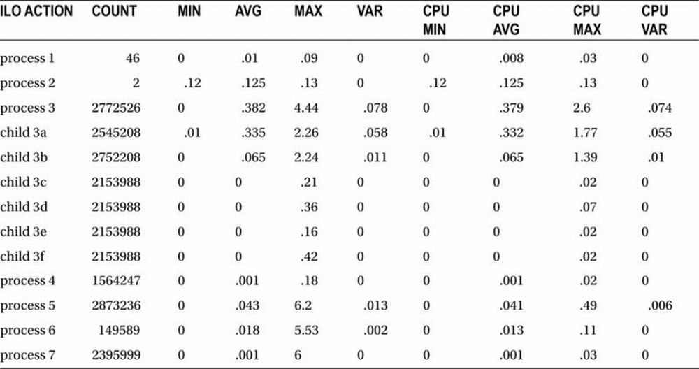
Although the numbers shown in the table aren’t particularly meaningful on their own, if you have this set of numbers representing code executions prior to a change and you have another set of numbers from the same server with the same dataset representing code execution after the code has been changed, you have definitive information regarding the impact of your code changes on the database. Imagine being able to repeat this test quickly and painlessly for subsequent code changes and configuration adjustments, and you just might begin to appreciate the potential of code instrumentation combined with repeatable, automated test processes.
Testing to Destruction
Testing a system to its breaking point can be one of the more entertaining aspects of software testing, and meetings to brainstorm all the possible ways to break the database are seldom dull. Early in my career, I developed and managed an Oracle Database application built using client/server technology. (Yes, this was long ago and far away.) The application itself was a problem tracking tool that allowed manufacturing workers to record issues they found and to send those problems to Engineering for review and correction. The initial report landed in Quality Engineering, where it was investigated and assigned to the appropriate Engineering group. As each Engineering department signed off on its work, the request moved on to the next group. The application was reasonably successful, so it ended up on many workstations throughout a very large facility.
If you ever want to see “testing to destruction” in action, try supporting a database application installed on the workstations of hundreds of electrical, hydraulic, and structural engineers. In a fairly short period of time, I learned that engineers do everything in their power to learn about the computers on their desks, and they considered breaking those computers and the applications on them to be an educational experience. I can’t say that I disagree with them; sometimes, taking something apart just so you can build it again really is the best way to understand the guts of the tool.
However, after several months of trying to support this very inquisitive group of people, I developed a new approach to discourage excessive tampering. By keeping a library of ghosted drives containing the standard workstation configuration with all the approved applications, I could replace the hard drive on a malfunctioning computer in less than ten minutes, and the engineer and I could both get back to work. Because everyone was expected to store their work on the server, no one could really object to my repair method. However, most engineers did not like losing their customized desktops, so they soon quit trying quite so hard to break things.
Although I loved to grumble at those engineers, I really owe them a very big thank you, for now whenever I need to think about how to test a server or application to destruction, all I need to do is think about those engineers and wonder what they would do. And never discount even the craziest ideas; if you can think of it, someone is likely to try it. As you work to identify your system’s weak links, consider everything on the following list, and then think of some more items:
- Data entry: What happens when a user or program interface sends the wrong kind of data or too much data?
- Task sequences: What happens when a user skips a step or performs the tasks out of order?
- Repeating/simultaneous executions: Can the user run the same process simultaneously? Will that action corrupt data or will it just slow down the process?
- Unbounded data ranges: Can the user request an unreasonable amount of data? What happens if the user enters an end range that is prior to the start range (such as requesting a report on sales from July 1, 2010, to June 30, 2010)?
- Resource usage: Excessive use of CPU, memory, temporary storage, and undo space can impact many users at the same time. Your DBA should limit usage with resource caps appropriately, but you still need to identify all the potential ways users and processes can grab more than their fair share.
I bet some of you could add some very interesting options for other ways to break systems. Can you also identify the ways to prevent those problems? Although finding the best correction is a bit harder and not as entertaining, every time you can make it difficult for a user to break your code, you create a more robust system—one that needs less support and less maintenance over the long run.
Every system has its own weakest links. When you’ve identified those weaknesses, assemble your unit tests into a test harness that pushes that resource beyond its limits so you can see how the system responds. In general, it seems that memory and IO usage are the primary stressors for a database system. However, lately I’ve been working on an Oracle 11g database with spatial functionality and, in this case, CPU processing is the system’s bottleneck. When we designed the system capacity tests, we made certain that the spatial processes would be tested to the extreme, and we measured internal database performance using the ILO data as shown in the last section. We also had external measurements of the total application and system performance, but having the ILO elapsed time data provided some unique advantages over other test projects in which I’ve participated.
First and foremost, the ILO data provide specific measurements of the time spent in the database. This makes it easier to troubleshoot performance issue that do show up, because you can tell quickly when the process is slow in the database and when it is not. A second advantage is that the recorded timestamps give a very specific indicator of exactly when a problem occurred, what other processes were running at the same time, and the specific sequencing of the application processes. With this information, you can easily identify the point when the system hits the knee in its performance curve. And because the elapsed time module in ILO uses dbms_utility.get_time and dbms_utility.get_cpu_time, you can record exactly how much time your process was active in the database and what portion of that time was spent on CPU.
These detailed performance data are also useful for troubleshooting, because the low-level timestamps assist in narrowing down the time frame for the problem. When you know the specific time frame you need to research, you can review a much smaller quantity of AWR or StatsPack data to determine what happened and find the answers quickly. When the window is small enough, any problem is visible almost immediately. We look at a specific case in the next section.
Troubleshooting through Instrumentation
Sometimes it can be difficult to identify the cause of small problems. When you don’t know the source of the problem, you also don’t know the potential impact the problem can have on your application. In one such case, developers had noticed timeouts from the database at random intervals, yet the process they suspected of causing the issue showed no sign of the errors and the database appeared to be working well below its potential.
About a week after a new test server was installed, a review of the ilo_elapsed_time table showed that most tasks were performing well, except there were two processes that had overrun the 30-second timeout clock on the application. The error numbers recorded on the tasks showed the front-end application had ended the connection; this message was consistent with a possible timeout, but it was not very helpful. The captured ILO data are shown in Table 15-2.
Table 15-2. Timeout Errors
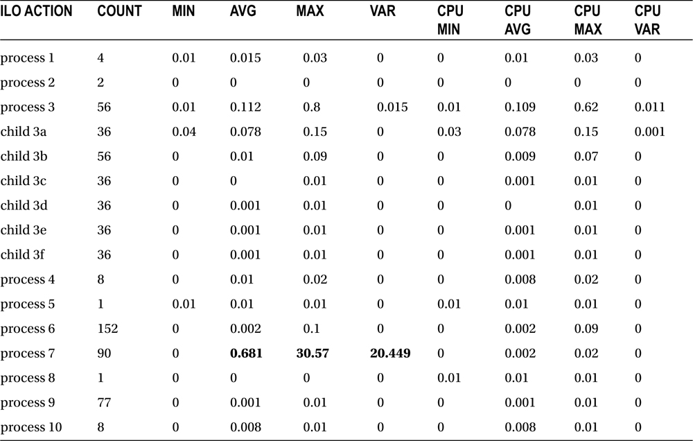
Take a look at process 7. Note that the maximum completion time does exceed 30 seconds, and the variance in processing times is relatively high when compared with other processes in the application. The process spends almost no time on CPU, so this is a problem worth investigating. Where is this time going? It’s also interesting to note that this was not a process that anyone would have expected to have a performance issue. Process 3 had been the target of previous timeout investigations; it has to perform considerably more work than process 7.
Next, let’s take a look at Table 15-3, which contains the results of a query looking for all cases when process 7 exceeded 30 seconds.
Table 15-3. Processes Exceeding 30 Seconds
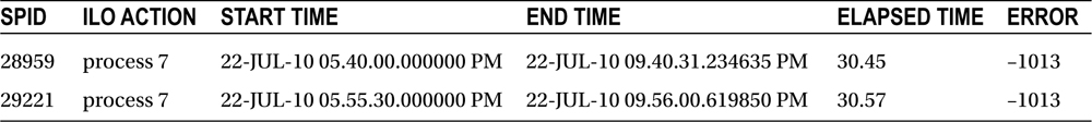
The start and stop times shown in Table 15-3 reflect the connection pool start and stop times, which is a much wider window than you need to troubleshoot this problem. Internal database and CPU clock times are also recorded in the ilo_elapsed_time table, and these are the values that are used to calculate the elapsed times as shown in Table 15-4. Table 15-4 also shows the sequential execution of the processes. Notice that process 7 was executed repeatedly within intervals of just a few seconds.
Table 15-4. Sequential Listing of Processes with Internal Clock Times
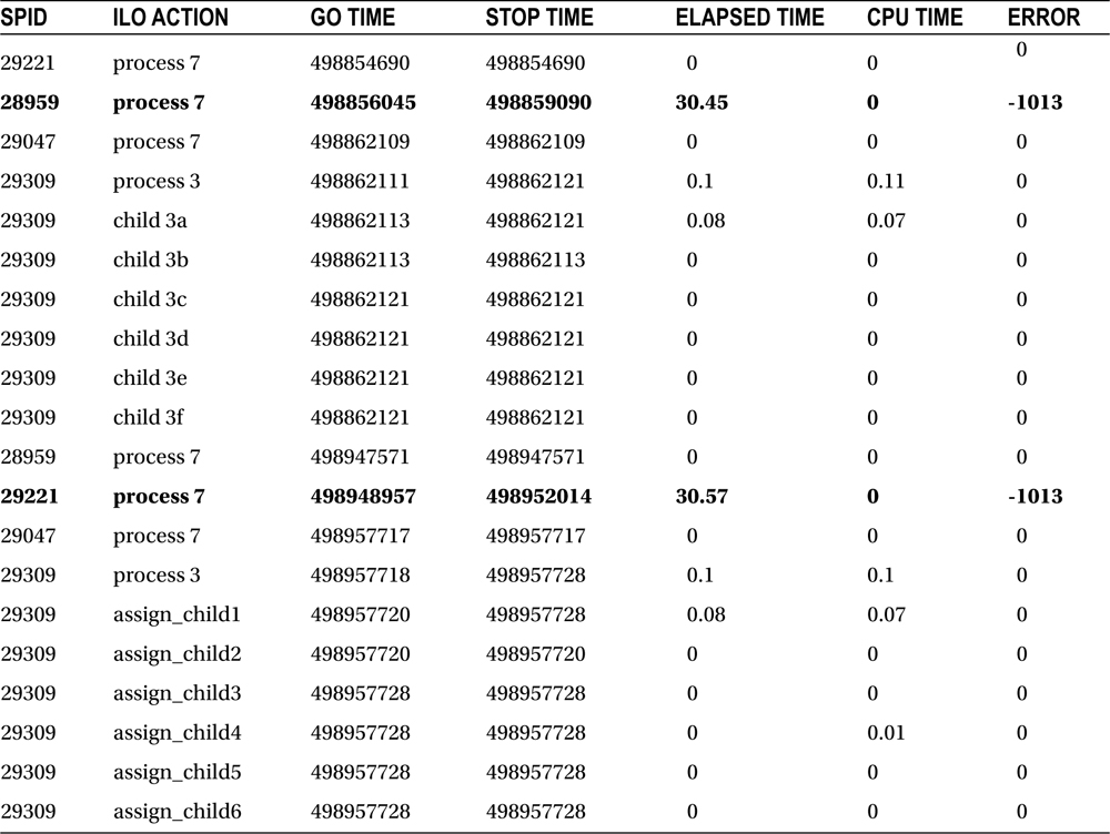
Looking at the two processes that exceeded 30 seconds, we can note a very small time frame when both errors occurred. The next step is to check the AWR for that particular time frame. On review of the AWR data shown in Listing 15-12, the problem is immediately clear.
Listing 15-12. AWR Output for One-Hour Time Frame
Top 5 Timed Foreground Events
∼∼∼∼∼∼∼∼∼∼∼∼∼∼∼∼∼∼∼∼∼∼∼∼∼∼∼∼∼
                                                 Avg
                                                wait  % DB
Event                           Waits Time(s)   (ms)  time Wait Class
------------------------------ ------ ------- ------ ----- ----------
enq: TX - row lock contention       2      61  30511  78.6 Application
DB CPU                                     12         15.0
SQL*Net break/reset to client  21,382       5      0   6.6 Application
log file sync                      32       0      1    .1 Commit
SQL*Net message to client      10,836       0      0    .0 Network
Between the series of events shown in Table 15-2 and the AWR output shown in Listing 15-12, the cause of the timeouts becomes clear. Process 7 was called two or even three times, when only one execution was necessary. If those calls came in fast enough, the second process attempted to update the same row, creating a lock and preventing the first process from committing. When process 1 could not commit in 30 seconds, the process terminated and the second (or third) process could save its changes successfully. Because the application has a built-in timeout, this problem is a minor one, and a self-correcting one at that.
Tables 15-1 to 15-4 show data from a newly installed server with only a few executions. I selected this particular dataset because it is easy to use as an example, but it does make it appear as if it would have been possible to spot this problem with almost any other troubleshooting tool. However, consider this: When these same data are reviewed on more active test servers over longer periods of time, timeouts for this process may occur on one day in any given month, and there are likely to be no more the four to six processes that exceed 30 seconds on that day. This process may execute hundreds of thousands of times over two or three months on a busy test server. And then there are test results like those shown in Table 15-1. In that case, the process is executed millions of times without a single timeout. Trying to spot this problem from an AWR report and then identifying the process that caused the application lock would take a bit more time with that many executions. And although this problem is not significant right now, it has the potential to cause the application to miss required performance targets. As a result of the data recorded by the instrumentation, the problem can be monitored and addressed before this happens.
Although this is a simple example, identifying these kinds of problems can be difficult, especially during typical development test cycles. Early in unit testing, tests are not usually executed in rapid succession, so some problems may not appear until later. And when testing has moved on to load testing, an occasionally longer running process or two may not be noticed among millions of executions. Yet, by using the ILO execution times to abbreviate the amount of AWR performance data that must be reviewed, problems like this can be identified and diagnosed in just a few moments. And although access to AWR and ASH data may not be available to you in all development environments, the instrumentation data you create are available.
Summary
I covered a wide range of information in this chapter, including execution plans and instrumentation, performance and failures, testing theory and practical application. Each of these topics could have been a chapter or even an entire book in its own right, which is why there are already many, many books out there that address these topics.
What I hope you take away from this chapter is the recognition that each system has its own strengths and limitations, so any testing and measurement approach should be customized to some extent for specific system needs and performance requirements. No single testing method can be completely effective for all systems, but the basic approach is fairly straightforward. Break down the work into measurable test modules, then measure, adjust, and measure again. Whenever possible, minimize the changes between test iterations, but keep the test realistic. You can test the functionality of your code with unit tests on a subset of the data, but testing performance requires a comparable amount of data on a comparably configured system. Verifying that a report runs exceptionally fast on a development server with little data and no other users doesn’t prove anything if that report is to be run on a multiuser data warehouse. Understanding what you need to measure and confirm is crucial to preparing an appropriate test plan. Be sure to consider testing and performance early during the code development process. This does not necessarily mean that you need to write a perfectly optimized piece of code right out of the gate, but you should be aware of the limitations your code is likely to face in production, then write the code accordingly. It also doesn’t hurt to have a few alternatives in your back pocket so you are prepared to optimize the code and measure it once again.