
![]()
Core SQL
Whether you’re relatively new to writing SQL or you’ve been writing it for years, learning to write “good” SQL is a process that requires a strong knowledge foundation of core syntax and concepts. This chapter provides a review of the core concepts of the SQL language and its capabilities, along with descriptions of the common SQL commands with which you should already be familiar. For those of you who have worked with SQL previously and have a good grasp on the basics, this chapter will be a brief refresher to prepare you for the more detailed treatment of SQL we examine in later chapters. If you’re a new SQL user, you may want to read Beginning Oracle SQL first to make sure you’re comfortable with the basics. Either way, Chapter 1 “level sets” you with a whirlwind tour of the five core SQL statements and provides a quick review of the tool we’ll be using to execute SQL: SQL*Plus.
The SQL Language
The SQL language was originally developed during the 1970s by IBM and was called Structured English Query Language, or SEQUEL. The language was based on the model for relational database management systems (RDBMSs) developed by E. F. Codd in 1969. The acronym was later shortened to SQL as a result of a trademark dispute. In 1986, the American National Standards Institute (ANSI) adopted SQL as a standard, and in 1987, the International Organization for Standardization (otherwise known as the ISO) did so as well. A piece of not-so-common knowledge is that the official pronunciation of the language was declared to be “ess queue ell” by ANSI. Most people, including me, still use the “see-qwell” pronunciation just because it flows a bit easier linguistically.
The purpose of SQL is simply to provide an interface to a database—in our case, Oracle. Every SQL statement is a command, or instruction, to the database. SQL differs from other programming languages such as C and Java in that it is intended to process data in sets, not individual rows. The language also doesn’t require that you provide instructions on how to navigate to the data; this happens transparently, under the covers. But, as you’ll see in the chapters ahead, knowing about your data and how and where they are stored is very important if you want to write efficient SQL in Oracle.
Although there are minor differences in how vendors (such as Oracle, IBM, and Microsoft) implement the core functionality of SQL, the skills you learn in one database transfer to another. Basically, you can use the same SQL statements to query, insert, update, and delete data and create, alter, and drop objects regardless of the database vendor.
Although SQL is the standard for use with various RDBMSs, it is not particularly relational in practice (I expand on this a bit later in the book). I recommend that you read C. J. Date’s book SQL and Relational Theory (O’Reilly Media, 2011) for a detailed review of how SQL and relational theory intersect. Keep in mind that the SQL language doesn’t always follow the relational model precisely; it doesn’t implement some elements of the relational model at all, and it implements other elements improperly. The fact remains that because SQL is based on this model, you must understand SQL and the relational model as well as know how to write SQL as correctly and efficiently as possible.
Interfacing to the Database
Numerous ways have been developed throughout the years for transmitting SQL to a database and getting results back. The native interface to the Oracle database is the Oracle Call Interface (OCI). The OCI powers the queries that are sent internally by the Oracle kernel to the database. You use the OCI any time you use one of Oracle’s tools, such as SQL*Plus or SQL Developer. Various other Oracle tools, including SQL*Loader, Data Pump, and Real Application Testing (RAT), use OCI as well as language-specific interfaces, such as Oracle JDBC-OCI, ODP.Net, Oracle Precompilers, Oracle ODBC, and the Oracle C++ Call Interface (OCCI) drivers.
When you use programming languages such as COBOL or C, the statements you write are known as embedded SQL statements and are preprocessed by a SQL preprocessor before the application program is compiled. Listing 1-1 shows an example of a SQL statement that could be used within a C/C++ block.
Listing 1-1. Embedded SQL Statement Used within a C/C++ Block
{
int a;
/* ... */
EXEC SQL SELECT salary INTO :a
    FROM hr.employees
   WHERE employee_id = 108;
/* ... */
printf("The salary is %d
", a);
/* ... */
}
Other tools, such as SQL*Plus and SQL Developer, are interactive tools. You enter and execute commands, and the output is displayed back to you. Interactive tools don’t require you to compile your code explicitly before running it; you simply enter the command you wish to execute. Listing 1-2 shows an example of using SQL*Plus to execute a statement.
Listing 1-2. Using SQL*Plus to Execute a SQL Statement
SQL> select  salary
  2  from    hr.employees
  3  where   employee_id = 108;

         SALARY
---------------
          12000
In this book, we’ll use SQL*Plus for our example listings for consistency’s sake, but keep in mind that whichever method or tool you use to enter and execute SQL statements, everything ultimately goes through the OCI. The bottom line is that the tool you use doesn’t matter; the native interface is the same for all.
Review of SQL*Plus
SQL*Plus is a command-line tool provided with every Oracle installation regardless of platform (Windows, Unix). It is used to enter and execute SQL commands and to display the resulting output in a text-only environment. The tool allows you to enter and edit commands, save and execute commands individually or via script files, and display the output in nicely formatted report form. To start SQL*Plus you simply start sqlplus from your host’s command prompt.
Connect to a Database
There are multiple ways to connect to a database from SQL*Plus. Before you can connect, however, you likely need to have entries for the databases to which you need to connect entered in the $ORACLE_HOME/network/admin/tnsnames.ora file. Two common ways to supply your connection information when you start SQL*Plus are shown in Listing 1-3; another is to use the SQL*Plus connect command after SQL*Plus starts, as shown in Listing 1-4.
Listing 1-3. Connecting to SQL*Plus from the Windows Command Prompt
$ sqlplus hr@ora12c

SQL*Plus: Release 12.1.0.1.0 Production on Tue May 7 12:32:36 2013

Copyright (c) 1982, 2013, Oracle.  All rights reserved.
Enter password:

Last Successful login time: Tue May 07 2013 12:29:09 -04:00
Connected to:
Oracle Database 12c Enterprise Edition Release 12.1.0.1.0 - 64bit Production
With the Partitioning, OLAP, Advanced Analytics and Real Application Testing options

SQL>
Listing 1-4. Connecting to SQL*Plus and Logging in to the Database from the SQL> Prompt
$ sqlplus /nolog

SQL*Plus: Release 12.1.0.1.0 Production on Tue May 7 12:34:21 2013

Copyright (c) 1982, 2013, Oracle.  All rights reserved.

SQL> connect hr@ora12c
Enter password:
Connected.
SQL>
When starting SQL*Plus using the 12c version, you will notice a new feature that displays your last login time by default. If you don’t want this to appear, simply use the option –nologintime.
To start SQL*Plus without being prompted to log in to a database, start SQL*Plus with the /nolog option.
Configuring the SQL*Plus Environment
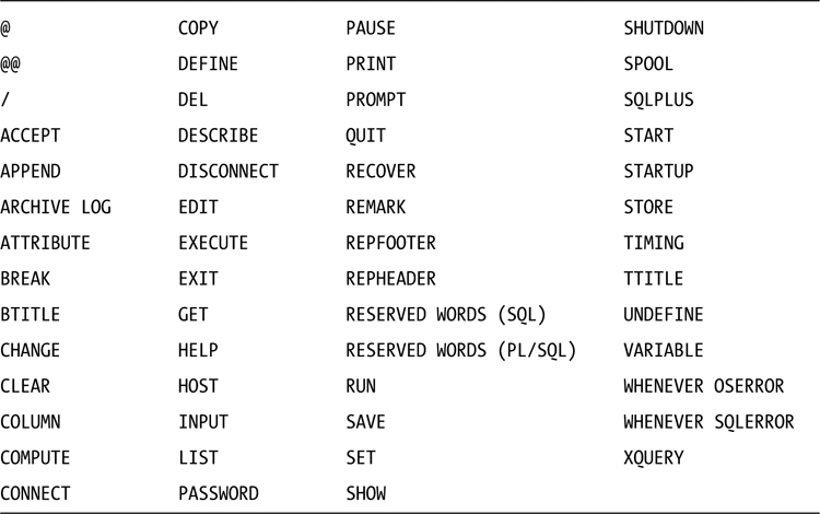
SQL*Plus has numerous commands that allow you to customize the working environment and display options. The SQL*Plus help data must be installed by the database administrator or it may not be available. There are three help script files found in $ORACLE_HOME/SQLPLUS/ADMIN/HELP/ that drop, create, and populate the SQL*Plus help tables: HLPBLD.SQL, HELPDROP.SQL, and HELPUS.SQL. Listing 1-5 shows the SQL*Plus commands available after entering the SQL*Plus help index command at the SQL> prompt.
Listing 1-5. SQL*Plus Command List
SQL> help index
Enter Help [topic] for help.
The set command is the primary command used for customizing your environment settings. Listing 1-6 shows the help text for the set command.
Listing 1-6. SQL*Plus SET Command
SQL> help set

 SET
 ---

 Sets a system variable to alter the SQL*Plus environment settings
 for your current session. For example, to:
     -   set the display width for data
     -   customize HTML formatting
     -   enable or disable printing of column headings
     -   set the number of lines per page

 SET system_variable value
 where system_variable and value represent one of the following clauses:

APPI[NFO]{OFF|ON|text}                       NEWP[AGE] {1|n|NONE}
ARRAY[SIZE] {15|n}                                  NULL text
AUTO[COMMIT] {OFF|ON|IMM[EDIATE]|n}          NUMF[ORMAT] format
AUTOP[RINT] {OFF|ON}                         NUM[WIDTH] {10|n}
AUTORECOVERY {OFF|ON}                        PAGES[IZE] {14|n}
AUTOT[RACE] {OFF|ON|TRACE[ONLY]}                    PAU[SE] {OFF|ON|text}
   [EXP[LAIN]] [STAT[ISTICS]]                RECSEP {WR[APPED]|EA[CH]|OFF}
BLO[CKTERMINATOR] {.|c|ON|OFF}                      RECSEPCHAR {_|c}
CMDS[EP] {;|c|OFF|ON}                        SERVEROUT[PUT] {ON|OFF}
COLSEP {_|text}                                             [SIZE {n | UNLIMITED}]
CON[CAT] {.|c|ON|OFF}                                [FOR[MAT]  {WRA[PPED] |
COPYC[OMMIT] {0|n}                                          WOR[D_WRAPPED] |
COPYTYPECHECK {ON|OFF}                               TRU[NCATED]}]
DEF[INE] {&|c|ON|OFF}                        SHIFT[INOUT] {VIS[IBLE] |
DESCRIBE [DEPTH {1|n|ALL}]                                         INV[ISIBLE]}
   [LINENUM {OFF|ON}] [INDENT {OFF|ON}]      SHOW[MODE] {OFF|ON}
ECHO {OFF|ON}                                       SQLBL[ANKLINES] {OFF|ON}
EDITF[ILE] file_name[.ext]                   SQLC[ASE] {MIX[ED] |
EMB[EDDED] {OFF|ON}                                  LO[WER] | UP[PER]}
ERRORL[OGGING] {ON|OFF}                             SQLCO[NTINUE] {> | text}
   [TABLE [schema.]tablename]                SQLN[UMBER] {ON|OFF}
   [TRUNCATE] [IDENTIFIER identifier]        SQLPLUSCOMPAT[IBILITY]
                                                            {x.y[.z]}
ESC[APE] {|c|OFF|ON}                        SQLPRE[FIX] {#|c}
ESCCHAR {@|?|%|$|OFF}                        SQLP[ROMPT] {SQL>|text}
EXITC[OMMIT] {ON|OFF}                        SQLT[ERMINATOR] {;|c|ON|OFF}
FEED[BACK] {6|n|ON|OFF}                             SUF[FIX] {SQL|text}
FLAGGER {OFF|ENTRY|INTERMED[IATE]|FULL}      TAB {ON|OFF}
FLU[SH] {ON|OFF}                                    TERM[OUT] {ON|OFF}
HEA[DING] {ON|OFF}                                  TI[ME] {OFF|ON}
HEADS[EP] {||c|ON|OFF}                       TIMI[NG] {OFF|ON}
INSTANCE [instance_path|LOCAL]                      TRIM[OUT] {ON|OFF}
LIN[ESIZE] {80|n}                                   TRIMS[POOL] {OFF|ON}
LOBOF[FSET] {1|n}                                   UND[ERLINE] {-|c|ON|OFF}
LOGSOURCE [pathname]                         VER[IFY] {ON|OFF}
LONG {80|n}                                                 WRA[P] {ON|OFF}
LONGC[HUNKSIZE] {80|n}                       XQUERY {BASEURI text|
MARK[UP] HTML [OFF|ON]                              ORDERING{UNORDERED|
   [HEAD text] [BODY text] [TABLE text]             ORDERED|DEFAULT}|
   [ENTMAP {ON|OFF}]                                NODE{BYVALUE|BYREFERENCE|
   [SPOOL {OFF|ON}]                                 DEFAULT}|
   [PRE[FORMAT] {OFF|ON}]                           CONTEXT text}
SQL>
Given the number of commands available, you can customize your environment easily to suit you best. One thing to keep in mind is that the set commands aren’t retained by SQL*Plus when you exit/close the tool. Instead of typing in each of the set commands you want to apply each time you use SQL*Plus, you can create a file named login.sql. There are actually two files that SQL*Plus reads by default each time you start it. The first is glogin.sql and it can be found in the directory $ORACLE_HOME/sqlplus/admin. If this file is found, it is read and the statements it contains are executed. This allows you to store the SQL*Plus commands and SQL statements that customize your experience across SQL*Plus sessions.
After reading glogin.sql, SQL*Plus looks for the login.sql file. This file must exist in either the directory from which SQL*Plus was started or in a directory included in the path to which the environment variable SQLPATH points. Any commands in login.sql will take precedence over those in glogin.sql. Since version 10g, Oracle reads both glogin.sql and login.sql each time you either start SQL*Plus or execute the connect command from within SQL*Plus. Prior to 10g, the login.sql script was only executed when SQL*Plus started. The contents of a common login.sql file are shown in Listing 1-7.
Listing 1-7. A Common login.sql File
SET LINES 3000
--Sets width of display line (default 80 characters)
SET PAGES 1000
-Sets number of lines per page (default 14 lines)
SET TIMING ON
--Sets display of elapsed time (default OFF)
SET NULL <null>
--Sets display of nulls to show <null> (default empty)
SET SQLPROMPT '&_user@&_connect_identifier> '
--Sets the prompt to show connected user and instance
Note the use of the variables _user and _connect_identifier in the SET SQLPROMPT command. These are two examples of predefined variables. You may use any of the following predefined variables in your login.sql file or in any other script file you may create:
- _connect_identifier (connection identifier used to make the database connection)
- _date (current date)
- _editor (the editor that is started when you use the EDIT command)
- _o_version (current version of the installed Oracle database)
- _o_release (full release number of the installed Oracle database)
- _privilege (privilege level of the current connection)
- _sqlplus_release (full release number of the installed SQL*Plus component)
- _user (username used to make the connection)
Executing Commands
There are two types of commands that can be executed within SQL*Plus: SQL statements and SQL*Plus commands. The SQL*Plus commands shown in Listings 1-5 and 1-6 are specific to SQL*Plus and can be used for customizing the environment and executing commands that are specific to SQL*Plus, such as DESCRIBE and CONNECT. Executing a SQL*Plus command requires only that you type the command at the prompt and press Enter. The command is executed automatically. On the other hand, to execute SQL statements, you must use a special character to indicate you wish to execute the entered command. You may use either a semicolon or a forward slash to do this. A semicolon may be placed directly at the end of the typed command or on a following blank line. The forward slash must be placed on a blank line to be recognized. Listing 1-8 shows how these two execution characters are used.
Listing 1-8. Execution Character Usage
SQL>select empno, deptno from scott.emp where ename = 'SMITH' ;
     EMPNO     DEPTNO
---------- ----------
      7369         20
SQL>select empno, deptno from scott.emp where ename = 'SMITH'
  2  ;
     EMPNO     DEPTNO
---------- ----------
      7369         20
SQL>select empno, deptno from scott.emp where ename = 'SMITH'
  2  /
     EMPNO     DEPTNO
---------- ----------
      7369         20
SQL>select empno, deptno from scott.emp where ename = 'SMITH'
  2
SQL>/
     EMPNO     DEPTNO
---------- ----------
      7369         20
SQL>select empno, deptno from scott.emp where ename = 'SMITH'/
  2
SQL>l
  1* select empno, deptno from scott.emp where ename = 'SMITH'/
SQL>/
select empno, deptno from scott.emp where ename = 'SMITH'/
                                                         *
ERROR at line 1:
ORA-00936: missing expression
Notice the fifth example that puts / at the end of the statement. The cursor moves to a new line instead of executing the command immediately. Then, if you press Enter again, the statement is entered into the SQL*Plus buffer but is not executed. To view the contents of the SQL*Plus buffer, the list command is used (abbreviated to l). If you then attempt to execute the statement in the buffer using /, which is how the / command is intended to be used, you get an error because, originally, you placed / at the end of the SQL statement line. The forward slash is not a valid SQL command and thus causes an error when the statement attempts to execute.
Another way to execute commands is to place them in a file. You can produce these files with the text editor of your choice outside of SQL*Plus or you may invoke an editor directly from SQL*Plus using the EDIT command. The EDIT command either opens a named file or creates a file if it doesn’t exist. The file must be in the default directory or you must specify the full path of the file. To set the editor to one of your choice, simply set the predefined _editor variable using the following command: define _editor='/<full path>/myeditor.exe'. Files with the extension .sql will execute without having to include the extension and can be run using either the @ or START command. Listing 1-9 shows the use of both commands.
Listing 1-9. Executing .sql Script Files
SQL> @list_depts
    DEPTNO DNAME          LOC
---------- -------------- -------------
        10 ACCOUNTING     NEW YORK
        20 RESEARCH       DALLAS
        30 SALES          CHICAGO
        40 OPERATIONS     BOSTON
SQL>
SQL> start list_depts
    DEPTNO DNAME          LOC
---------- -------------- -------------
        10 ACCOUNTING     NEW YORK
        20 RESEARCH       DALLAS
        30 SALES          CHICAGO
        40 OPERATIONS     BOSTON
SQL>
SQL>l
  1* select * from scott.dept
SQL>
SQL*Plus has many features and options—far too many to cover here. For what we need in this book, the previous overview should suffice. However, the Oracle documentation provides guides for SQL*Plus use and there are numerous books, including Beginning Oracle SQL (as mentioned earlier), that go in to more depth if you’re interested.
The Five Core SQL Statements
The SQL language contains many different statements. In your professional career you may end up using just a small percentage of what is available to you. But isn’t that the case with almost any product you use? I once heard a statistic that most people use 20 percent or less of the functionality available in the software products or programming languages they use regularly. I don’t know whether this is actually true, but in my experience, it seems fairly accurate. I have found the same basic SQL statement formats in use within most applications for almost 20 years. Very few people ever use everything SQL has to offer—and they often implement improperly those features they do use frequently. Obviously, we will not be able to cover all the statements and their options found in the SQL language. This book is intended to provide you with deeper insight into the most commonly used statements and to help you understand how to apply them more effectively.
In this book, we will examine five of the most frequently used SQL statements. These statements are SELECT, INSERT, UPDATE, DELETE, and MERGE. Although we’ll address each of these core statements in some fashion, our focus is primarily on the SELECT statement. Developing a good command of these five statements will provide a strong foundation for your day-to-day work with the SQL language.
The SELECT statement is used to retrieve data from one or more tables or other database objects. You should already be familiar with the basics of the SELECT statement, so instead of reviewing the statement from the beginner’s point of view, I want to review how a SELECT statement processes logically. You should have already learned the basic clauses that form a common SELECT statement, but to build the foundation mind-set you need to write well-formed and efficient SQL consistently, you need to understand how SQL processes.
How a query statement is processed logically may be quite different from its actual physical processing. The Oracle cost-based optimizer (CBO) is responsible for generating the actual execution plan for a query, and we will examine what the optimizer does, and how it does it and why. For now, note that the optimizer determines how to access tables and the order in which to process them, and how to join multiple tables and apply filters. The logical order of query processing occurs in a very specific order. However, the steps the optimizer chooses for the physical execution plan can end up actually processing the query in a very different order. Listing 1-10 shows a query stub that contains the main clauses of a SELECT statement with step numbers assigned to each clause in the order it is processed logically.
Listing 1-10. Logical Query Processing Order
5      SELECT  <column list>
1      FROM            <source object list>
1.1    FROM            <left source object> <join type>
                   JOIN <right source object> ON <on predicates>
2      WHERE           <where predicates>
3      GROUP BY        <group by expression(s)>
4      HAVING          <having predicates>
6      ORDER BY        <order by list>
You should notice right away that SQL differs from other programming languages in that the first written statement (SELECT) is not the first line of code that is processed; the FROM clause is processed first. Note that I show two different FROM clauses in this listing. The one marked 1.1 is provided to show the difference when ANSI syntax is used. It may be helpful to imagine that each step in the processing order creates a temporary dataset. As each step is processed, the dataset is manipulated until a final result is formulated. It is this final result set of data that the query returns to the caller.
To walk through each part of the SELECT statement in more detail, you need to use the query in Listing 1-11 that returns a result set that contains a list of female customers that have placed more than four orders.
Listing 1-11. Female Customers Who Have Placed More Than Four Orders
SQL> select c.customer_id, count(o.order_id) as orders_ct
  2  from oe.customers c
  3  join oe.orders o
  4  on c.customer_id = o.customer_id
  5  where c.gender = 'F'
  6  group by c.customer_id
  7  having count(o.order_id) > 4
  8  order by orders_ct, c.customer_id
  9  /
CUSTOMER_ID  ORDERS_CT
----------- ----------
        146          5
        147          5
The FROM Clause
The FROM clause lists the source objects from which data are selected. This clause can contain tables, views, materialized views, partitions, or subpartitions, or may specify a subquery that identifies objects. If multiple source objects are used, this logical processing phase also applies to each join type and ON predicate. We explore join types in more detail later, but note that, as joins are processed, they occur in the following order:
- Cross join, also called a Cartesian product
- Inner join
- Outer join
In the example query in Listing 1-11, the FROM clause lists two tables: customers and orders. They are joined on the customer_id column. So, when this information is processed, the initial dataset that is produced by the FROM clause includes rows in which customer_id matches in both tables. The result set contains 105 rows at this point. To verify this is true, simply execute only the first four lines of the example query, as shown in Listing 1-12.
Listing 1-12. Partial Query Execution through the FROM Clause Only
SQL> select c.customer_id cust_id, o.order_id ord_id, c.gender
  2  from oe.customers c
  3  join oe.orders o
  4  on c.customer_id = o.customer_id;

CUST_ID ORD_ID G  CUST_ID ORD_ID G  CUST_ID ORD_ID G
------- ------ -  ------- ------ -  ------- ------ -
    147   2450 F      101   2430 M      109   2394 M
    147   2425 F      101   2413 M      116   2453 M
    147   2385 F      101   2447 M      116   2428 M
    147   2366 F      101   2458 M      116   2369 M
    147   2396 F      102   2431 M      116   2436 M
    148   2451 M      102   2414 M      117   2456 M
    148   2426 M      102   2432 M      117   2429 M
    148   2386 M      102   2397 M      117   2370 M
    148   2367 M      103   2437 F      117   2446 M
    148   2406 M      103   2415 F      118   2457 M
    149   2452 M      103   2433 F      118   2371 M
    149   2427 M      103   2454 F      120   2373 M
    149   2387 M      104   2438 F      121   2374 M
    149   2368 M      104   2416 F      122   2375 M
    149   2434 M      104   2355 F      123   2376 F
    150   2388 M      104   2354 F      141   2377 M
    151   2389 M      105   2439 F      143   2380 M
    152   2390 M      105   2417 F      144   2445 M
    153   2391 M      105   2356 F      144   2422 M
    154   2392 F      105   2358 F      144   2382 M
    155   2393 M      106   2441 M      144   2363 M
    156   2395 F      106   2418 M      144   2435 M
    157   2398 M      106   2359 M      145   2448 M
    158   2399 M      106   2381 M      145   2423 M
    159   2400 M      107   2442 F      145   2383 M
    160   2401 M      107   2419 F      145   2364 M
    161   2402 M      107   2360 F      145   2455 M
    162   2403 M      107   2440 F      119   2372 M
    163   2404 M      108   2443 M      142   2378 M
    164   2405 M      108   2420 M      146   2449 F
    165   2407 M      108   2361 M      146   2424 F
    166   2408 F      108   2357 M      146   2384 F
    167   2409 M      109   2444 M      146   2365 F
    169   2411 F      109   2421 M      146   2379 F
    170   2412 M      109   2362 M      168   2410 M
105 rows selected.
![]() Note I formatted the result of this output manually to make it fit nicely on the page. The actual output was displayed over 105 separate lines.
Note I formatted the result of this output manually to make it fit nicely on the page. The actual output was displayed over 105 separate lines.
The WHERE Clause
The WHERE clause provides a way to limit conditionally the rows emitted to the query’s final result set. Each condition, or predicate, is entered as a comparison of two values or expressions. The comparison matches (evaluates to TRUE) or does not match (evaluates to FALSE). If the comparison is FALSE, then the row is not included in the final result set.
I need to digress just a bit to cover an important aspect of SQL related to this step. Actually, the possible values of a logical comparison in SQL are TRUE, FALSE, and UNKNOWN. The UNKNOWN value occurs when a null is involved. Nulls compared with anything or nulls used in expressions evaluate to null, or UNKNOWN. A null represents a missing value and can be confusing because of inconsistencies in how nulls are treated within different elements of the SQL language. I address how nulls affect the execution of SQL statements throughout the book, although I mention the topic only briefly at this point. What I stated previously is still basically true; comparisons return either TRUE or FALSE. What you’ll find is that when a null is involved in a filter comparison, it is treated as if it is FALSE.
In our example, there is a single predicate used to limit the result only to females who have placed orders. If you review the intermediate result after the FROM clause was processed (see Listing 1-12), you’ll note that only 31 of the 105 rows were placed by female customers (gender = ‘F’). Therefore, after the WHERE clause is applied, the intermediate result set is reduced from 105 rows to 31 rows.
After the WHERE clause is applied, the detailed result set is ready. Note that I use the phrase detailed result set. What I mean is the rows that satisfy the query requirements are now available. Other clauses may be applied (GROUP BY, HAVING) that aggregate and limit the final result set further that the caller receives, but it is important to note that, at this point, all the data your query needs to compute the final answer are available.
The WHERE clause is intended to restrict, or reduce, the result set. The less restrictions you include, the more data your final result set contains. The more data you need to return, the longer the query takes to execute.
The GROUP BY Clause
The GROUP BY clause aggregates the filtered result set available after processing the FROM and WHERE clauses. The selected rows are grouped by the expression(s) listed in this clause to produce a single row of summary information for each group. You may group by any column of any object listed in the FROM clause, even if you don’t intend to display that column in the list of output columns. Conversely, any nonaggregate column in the select list must be included in the GROUP BY expression.
There are two additional operations that can be included in a GROUP BY clause: ROLLUP and CUBE. The ROLLUP operation is used to produce subtotal values. The CUBE operation is used to produce cross-tabulation values. If you use either of these operations, you get more than one row of summary information. Both these operations are discussed in detail in Chapter 7.
In the example query, the requested grouping is customer_id. This means that there is only one row for each distinct customer_id. Of the 31 rows that represent the females who placed orders that made it through the WHERE clause processing, there are 11 distinct customer_id values, as shown in Listing 1-13.
Listing 1-13. Partial Query Execution through the GROUP BY Clause
SQL> select c.customer_id, count(o.order_id) as orders_ct
  2  from oe.customers c
  3  join oe.orders o
  4  on c.customer_id = o.customer_id
  5 where gender = 'F'
  6 group by c.customer_id;

CUSTOMER_ID  ORDERS_CT
----------- ----------
        156          1
        123          1
        166          1
        154          1
        169          1
        105          4
        103          4
        107          4
        104          4
        147          5
        146          5
11 rows selected.
Notice that the output from the query, although grouped, is not ordered. The display makes it appear as though the rows are ordered by order_ct, but this is more coincidence and not guaranteed behavior. This is an important item to remember; the GROUP BY clause does not ensure ordering of data. If you want the list to display in a specific order, you have to specify an ORDER BY clause.
The HAVING Clause
The HAVING clause restricts the grouped summary rows to those for which the condition(s) in the clause are TRUE. Unless you include a HAVING clause, all summary rows are returned. The GROUP BY and HAVING clauses are actually interchangeable positionally (it doesn’t matter which one comes first). However, it seems to make more sense to code them with the GROUP BY clause first, because GROUP BY is processed logically first. Essentially, the HAVING clause is a second WHERE clause that is evaluated after GROUP BY occurs, and is used to filter on grouped values. Because the WHERE clause is applied before the GROUP BY occurs, you cannot filter grouped results in the WHERE clause; you must use the HAVING clause instead.
In our example query, the HAVING clause, HAVING COUNT(o.order_id) > 4, limits the grouped result data of 11 rows down to two rows. You can confirm this by reviewing the list of rows returned after GROUP BY is applied, as shown in Listing 1-13. Note that only customers 146 and 147 have placed more than four orders. The two rows that make up the final result set are now ready.
The SELECT List
The SELECT list is where the columns included in the final result set from your query are provided. A column can be an actual column from a table, an expression, or even the result of a SELECT statement, as shown in Listing 1-14.
Listing 1-14. Example Query Showing SELECT List Alternatives
SQL> select c.customer_id, c.cust_first_name||' '||c.cust_last_name,
  2  (select e.last_name from hr.employees e where e.employee_id = c.account_mgr_id) acct_mgr)
  3  from oe.customers c;

    CUSTOMER_ID CUST_NAME                                 ACCT_MGR
--------------- ----------------------------------------- --------------
            147 Ishwarya Roberts                          Russell
            148 Gustav Steenburgen                        Russell
...
            931 Buster Edwards                            Cambrault
            981 Daniel Gueney                             Cambrault
319 rows selected.
When another SELECT statement is used to produce the value of a column, the query must return only one row and one column value. These types of subqueries are referred to as scalar subqueries. Although this can be very useful syntax, keep in mind that the scalar subquery is executed once for each row in the result set. There are optimizations available that may eliminate some duplicate executions of the subquery, but the worst-case scenario is that each row requires this scalar subquery to be executed. Imagine the possible overhead involved if your result set had thousands, or millions, of rows! I review scalar subqueries later in the book and discuss how to use them optimally.
Another option you may need to use in the SELECT list is the DISTINCT clause. The example provided here doesn’t use it, but I want to mention it briefly. The DISTINCT clause causes duplicate rows to be removed from the dataset produced after the other clauses have been processed.
After the SELECT list is processed, you now have the final result set for your query. The only thing that remains to be done, if it is included, is to sort the result set into a desired order.
The ORDER BY Clause
The ORDER BY clause is used to order the final set of rows returned by the statement. In this case, the requested sort order was to be by orders_ct and customer_id. The orders_ct column is the value computed using the COUNT aggregate function in the GROUP BY clause. As shown in Listing 1-13, there are two customers that each placed more than four orders. Because each customer placed five orders, the order_ct is the same, so the second ordering column determines the final display order. As shown in Listing 1-15, the final sorted output of the query is a two-row dataset ordered by customer_id.
Listing 1-15. Example Query Final Output
SQL> select c.customer_id, count(o.order_id) as orders_ct
  2  from oe.customers c
  3  join oe.orders o
  4  on c.customer_id = o.customer_id
  5  where c.gender = 'F'
  6  group by c.customer_id
  7  having count(o.order_id) > 4
  8  order by orders_ct, c.customer_id
  9  /
CUSTOMER_ID  ORDERS_CT
----------- ----------
        146          5
        147          5
When ordered output is requested, Oracle must take the final set of data after all other clauses have been processed and sort them as specified. The size of the data that needs to be sorted is important. When I say size, I mean total bytes of data in the result set. To estimate the size of the dataset, multiply the number of rows by the number of bytes per row. The bytes per row are determined by summing the average column lengths of each of the columns in the SELECT list.
The example query requests only the customer_id and orders_ct column values in the SELECT list. Let’s use ten as our estimated bytes-per-row value. In Chapter 6, I show you where to find the optimizer’s estimate for this value. So, given that we only have two rows in the result set, the sort size is actually quite small, approximately 20 bytes. Remember, this is only an estimate, but the estimate is an important one.
Small sorts should be accomplished entirely in memory whereas large sorts may have to use temporary disk space to complete the sort. As you may likely deduce, a sort that occurs in memory is faster than a sort that must use disk. Therefore, when the optimizer estimates the effect of sorting data, it has to consider how big the sort is to adjust how to accomplish getting the query result in the most efficient way. In general, consider sorts as a fairly expensive overhead to your query processing time, particularly if the size of your result set is large.
The INSERT statement is used to add rows to a table, partition, or view. Rows can be inserted in either a single-table or multitable method. A single-table insert inserts values into one row of one table either by specifying the values explicitly or by retrieving the values using a subquery. The multitable insert inserts rows into one or more tables and computes the row values it inserts by retrieving the values using a subquery.
Single-Table Inserts
The first example in Listing 1-16 illustrates a single-table insert using the VALUES clause. Each column value is entered explicitly. The column list is optional if you include values for each column defined in the table. However, if you only want to provide values for a subset of the columns, you must specify the column names in the column list. A good practice is to include the column list regardless of whether you specify values for all the columns. Doing so acts to self-document the statement and also helps reduce possible errors that might occur in the future should someone add a new column to the table.
Listing 1-16. Single-Table Insert
SQL> insert into hr.jobs (job_id, job_title, min_salary, max_salary)
  2  values ('IT_PM', 'Project Manager', 5000, 11000) ;
1 row created.

SQL> insert into scott.bonus (ename, job, sal)
  2  select ename, job, sal * .10
  3  from scott.emp;

14 rows created.
The second example in Listing 1-16 illustrates an insert using a subquery, which is a very flexible option for inserting rows. The subquery can be written to return one or more rows. Each row returned is used to supply column values for the new rows to be inserted. The subquery can be as simple or as complex as needed to satisfy your needs. In this example, we use the subquery to compute a 10 percent bonus for each employee based on his or her current salary. The bonus table actually has four columns, but we only populate three of them with this insert. The comm column isn’t populated with a value from the subquery and we do not include it in the column list. Because we don’t include this column, the value for it is null. Note that if the comm column had a NOT NULL constraint, you would get a constraint error and the statement would fail.
Multitable Inserts
The multitable insert example in Listing 1-17 illustrates how rows returned from a single subquery can be used to insert rows into more than one table. We start with three tables: small_customers, medium_customers, and large_customers. Let’s populate these tables with customer data based on the total amount of orders a customer has placed. The subquery sums the order_total column for each customer, and then the insert places a row conditionally in the proper table based on whether the customer is considered to be small (less than $10,000 of total orders), medium (between $10,000 and $99,999.99), or large (greater than or equal to $100,000).
Listing 1-17. Multitable Insert
SQL> select * from small_customers ;

no rows selected

SQL> select * from medium_customers ;

no rows selected

SQL> select * from large_customers ;

no rows selected

SQL> insert all
  2  when sum_orders < 10000 then
  3  into small_customers
  4  when sum_orders >= 10000 and sum_orders < 100000 then
  5  into medium_customers
  6  else
  7  into large_customers
  8  select customer_id, sum(order_total) sum_orders
  9  from oe.orders
 10  group by customer_id ;

47 rows created.

SQL> select * from small_customers ;

CUSTOMER_ID SUM_ORDERS
----------- ----------
        120        416
        121       4797
        152     7616.8
        157     7110.3
        160      969.2
        161        600
        162        220
        163        510
        164       1233
        165       2519
        166        309
        167         48

12 rows selected.

SQL> select * from medium_customers ;

CUSTOMER_ID SUM_ORDERS
----------- ----------
        102    69211.4
        103    20591.4
        105    61376.5
        106    36199.5
        116      32307
        119    16447.2
        123    11006.2
        141    38017.8
        142    25691.3
        143    27132.6
        145    71717.9
        146    88462.6
        151      17620
        153    48070.6
        154      26632
        155    23431.9
        156      68501
        158    25270.3
        159    69286.4
        168      45175
        169    15760.5
        170      66816

22 rows selected.

SQL> select * from large_customers ;

CUSTOMER_ID SUM_ORDERS
----------- ----------
        101   190395.1
        104   146605.5
        107   155613.2
        108   213399.7
        109   265255.6
        117   157808.7
        118   100991.8
        122   103834.4
        144   160284.6
        147   371278.2
        148   185700.5
        149   403119.7
        150   282694.3

13 rows selected.
Note the use of the ALL clause after the INSERT keyword. When ALL is specified, the statement performs unconditional multitable inserts, which means that each WHEN clause is evaluated for each row returned by the subquery regardless of the outcome of a previous condition. Therefore, you need to be careful about how you specify each condition. For example, if I had used WHEN sum_orders < 100000 instead of the range I specified, the medium_customers table would have included the rows that were also inserted into small_customers.
Specify the FIRST option to cause each WHEN to be evaluated in the order it appears in the statement and to skip subsequent WHEN clause evaluations for a given subquery row. The key is to remember which option, ALL or FIRST, best meets your needs, then use the one most suitable.
The UPDATE Statement
The UPDATE statement is used to change the column values of existing rows in a table. The syntax for this statement is composed of three parts: UPDATE, SET, and WHERE. The UPDATE clause specifies the table to update. The SET clause specifies which columns are changed and the modified values. The WHERE clause is used to filter conditionally which rows are updated. This clause is optional; if it is omitted, the update operation is applied to all rows of the specified table.
Listing 1-18 demonstrates several different ways an UPDATE statement can be written. First, I create a duplicate of the employees table called employees2, then I execute several different updates that accomplish basically the same task: the employees in department 90 are updated to have a 10 percent salary increase and, in the case of example 5, the commission_pct column is also updated. The following list includes the different approaches taken:
- Example 1: Update a single column value using an expression.
- Example 2: Update a single column value using a subquery.
- Example 3: Update a single column using a subquery in the WHERE clause to determine which rows to update.
- Example 4: Update a table using a SELECT statement to define the table and the column values.
- Example 5: Update multiple columns using a subquery.
Listing 1-18. UPDATE Statement Examples
SQL> -- create a duplicate employees table
SQL> create table employees2 as select * from employees ;
Table created.

SQL> -- add a primary key
SQL> alter table employees2
  1  add constraint emp2_emp_id_pk primary key (employee_id) ;

Table altered.

SQL> -- retrieve list of employees in department 90
SQL> select employee_id, last_name, salary
  2  from employees where department_id = 90 ;

    EMPLOYEE_ID LAST_NAME                          SALARY
--------------- ------------------------- ---------------
            100 King                                24000
            101 Kochhar                             17000
            102 De Haan                             17000

3 rows selected.

SQL> -- Example 1: Update a single column value using an expression

SQL> update employees2
  2  set salary = salary * 1.10 -- increase salary by 10%
  3  where department_id = 90 ;

3 rows updated.

SQL> commit ;

Commit complete.

SQL> select employee_id, last_name, salary
  2  from employees2 where department_id = 90 ;

EMPLOYEE_ID LAST_NAME  SALARY
----------- ---------- ------
        100 King        26400 -- previous value 24000
        101 Kochhar     18700 -- previous value 17000
        102 De Haan     18700 -- previous value 17000

3 rows selected.

SQL> -- Example 2: Update a single column value using a subquery

SQL> update employees
  2  set salary = (select employees2.salary
  3                  from employees2
  4                 where employees2.employee_id = employees.employee_id
  5                   and employees.salary != employees2.salary)
  6  where department_id = 90 ;

3 rows updated.

SQL> select employee_id, last_name, salary
  2  from employees where department_id = 90 ;

    EMPLOYEE_ID LAST_NAME                          SALARY
--------------- ------------------------- ---------------
            100 King                                26400
            101 Kochhar                             18700
            102 De Haan                             18700

3 rows selected.

SQL> rollback ;

Rollback complete.

SQL> -- Example 3: Update single column using subquery in
SQL> -- WHERE clause to determine which rows to update

SQL> update employees
  2  set salary = salary * 1.10
  3  where department_id in (select department_id
  4                            from departments
  5                           where department_name = 'Executive') ;

3 rows updated.
SQL> select employee_id, last_name, salary
  2  from employees
  3  where department_id in (select department_id
  4                            from departments
  5                           where department_name = 'Executive') ;

    EMPLOYEE_ID LAST_NAME                          SALARY
--------------- ------------------------- ---------------
            100 King                                26400
            101 Kochhar                             18700
            102 De Haan                             18700

3 rows selected.
SQL> rollback ;
Rollback complete.

SQL> -- Example 4: Update a table using a SELECT statement
SQL> -- to define the table and column values

SQL> update (select e1.salary, e2.salary new_sal
  2            from employees e1, employees2 e2
  3           where e1.employee_id = e2.employee_id
  4             and e1.department_id = 90)
  5  set salary = new_sal;

3 rows updated.

SQL> select employee_id, last_name, salary, commission_pct
  2  from employees where department_id = 90 ;

    EMPLOYEE_ID LAST_NAME                          SALARY  COMMISSION_PCT
--------------- ------------------------- --------------- ---------------
            100 King                                26400
            101 Kochhar                             18700
            102 De Haan                             18700

3 rows selected.
SQL> rollback ;
Rollback complete.

SQL> -- Example 5: Update multiple columns using a subquery

SQL> update employees
  2  set (salary, commission_pct) = (select employees2.salary, .10 comm_pct
  3                  from employees2
  4                 where employees2.employee_id = employees.employee_id
  5                   and employees.salary != employees2.salary)
  6  where department_id = 90 ;

3 rows updated.
SQL> select employee_id, last_name, salary, commission_pct
  2  from employees where department_id = 90 ;

    EMPLOYEE_ID LAST_NAME                          SALARY  COMMISSION_PCT
--------------- ------------------------- --------------- ---------------
            100 King                                26400              .1
            101 Kochhar                             18700              .1
            102 De Haan                             18700              .1

3 rows selected.

SQL> rollback ;

Rollback complete.

SQL>
The DELETE Statement
The DELETE statement is used to remove rows from a table. The syntax for this statement is composed of three parts: DELETE, FROM, and WHERE. The DELETE keyword stands alone. Unless you decide to use a hint, which we examine later, there are no other options associated with the DELETE keyword. The FROM clause identifies the table from which rows are to be deleted. As the examples in Listing 1-19 demonstrate, the table can be specified directly or via a subquery. The WHERE clause provides any filter conditions to help determine which rows are deleted. If the WHERE clause is omitted, the DELETE operation deletes all rows in the specified table.
Listing 1-19. DELETE Statement Examples
SQL> select employee_id, department_id, last_name, salary
  2  from employees2
  3  where department_id = 90;
    EMPLOYEE_ID   DEPARTMENT_ID LAST_NAME                          SALARY
--------------- --------------- ------------------------- ---------------
            100              90 King                                26400
            101              90 Kochhar                             18700
            102              90 De Haan                             18700

3 rows selected.
SQL> -- Example 1: Delete rows from specified table using
SQL> -- a filter condition in the WHERE clause
SQL> delete from employees2
  2  where department_id = 90;

3 rows deleted.

SQL> select employee_id, department_id, last_name, salary
  2  from employees2
  3  where department_id = 90;

no rows selected

SQL> rollback;

Rollback complete.

SQL> select employee_id, department_id, last_name, salary
  2  from employees2
  3  where department_id = 90;

    EMPLOYEE_ID   DEPARTMENT_ID LAST_NAME                          SALARY
--------------- --------------- ------------------------- ---------------
            100              90 King                                26400
            101              90 Kochhar                             18700
            102              90 De Haan                             18700

3 rows selected.

SQL> -- Example 2: Delete rows using a subquery in the FROM clause
SQL> delete from (select * from employees2 where department_id = 90);

3 rows deleted.

SQL> select employee_id, department_id, last_name, salary
  2  from employees2
  3  where department_id = 90;

no rows selected

SQL> rollback;

Rollback complete.

SQL> select employee_id, department_id, last_name, salary
  2  from employees2
  3  where department_id = 90;

    EMPLOYEE_ID   DEPARTMENT_ID LAST_NAME                          SALARY
--------------- --------------- ------------------------- ---------------
            100              90 King                                26400
            101              90 Kochhar                             18700
            102              90 De Haan                             18700

3 rows selected.

SQL> -- Example 3: Delete rows from specified table using
SQL> -- a subquery in the WHERE clause
SQL> delete from employees2
  2  where department_id in (select department_id
  3                       from departments
  4                      where department_name = 'Executive'),

3 rows deleted.

SQL> select employee_id, department_id, last_name, salary
  2  from employees2
  3  where department_id = 90;

no rows selected

SQL> rollback;

Rollback complete.

SQL>
Listing 1-19 demonstrates several different ways a DELETE statement can be written. Note that I am using the employees2 table created in Listing 1-18 for these examples. The following are the different delete methods that you can use:
- Example 1: Delete rows from a specified table using a filter condition in the WHERE clause.
- Example 2: Delete rows using a subquery in the FROM clause.
- Example 3: Delete rows from a specified table using a subquery in the WHERE clause.
The MERGE Statement
The MERGE statement is a single command that combines the ability to update or insert rows into a table by deriving conditionally the rows to be updated or inserted from one or more sources. It is used most frequently in data warehouses to move large amounts of data, but its use is not limited only to data warehouse environments. The big value-add this statement provides is that you have a convenient way to combine multiple operations into one, which allows you to avoid issuing multiple INSERT, UPDATE, and DELETE statements. And, as you’ll see later in the book, if you can avoid doing work you really don’t have to do, your response times will likely improve.
The syntax for the MERGE statement is as follows:
MERGE <hint>
INTO <table_name>
USING <table_view_or_query>
ON (<condition>)
WHEN MATCHED THEN <update_clause>
DELETE <where_clause>
WHEN NOT MATCHED THEN <insert_clause>
[LOG ERRORS <log_errors_clause> <reject limit <integer | unlimited>];
To demonstrate the use of the MERGE statement, Listing 1-20 shows how to create a test table and then insert or update rows appropriately into that table based on the MERGE conditions.
Listing 1-20. MERGE Statement Example
SQL> create table dept60_bonuses
  2  (employee_id       number
  3  ,bonus_amt         number);

Table created.

SQL> insert into dept60_bonuses values (103, 0);

1 row created.

SQL> insert into dept60_bonuses values (104, 100);

1 row created.

SQL> insert into dept60_bonuses values (105, 0);

1 row created.

SQL> commit;

Commit complete.

SQL> select employee_id, last_name, salary
  2  from employees
  3  where department_id = 60 ;

    EMPLOYEE_ID LAST_NAME                          SALARY
--------------- ------------------------- ---------------
            103 Hunold                               9000
            104 Ernst                                6000
            105 Austin                               4800
            106 Pataballa                            4800
            107 Lorentz                              4200

5 rows selected.

SQL> select * from dept60_bonuses;

    EMPLOYEE_ID       BONUS_AMT
--------------- ---------------
            103               0
            104             100
            105               0

3 rows selected.

SQL> merge into dept60_bonuses b
  2  using (
  3    select employee_id, salary, department_id
  4    from employees
  5    where department_id = 60) e
  6  on (b.employee_id = e.employee_id)
  7  when matched then
  8    update set b.bonus_amt = e.salary * 0.2
  9     where b.bonus_amt = 0
 10    delete where (e.salary > 7500)
 11  when not matched then
 12    insert (b.employee_id, b.bonus_amt)
 13    values (e.employee_id, e.salary * 0.1)
 14    where (e.salary < 7500);

4 rows merged.

SQL> select * from dept60_bonuses;

    EMPLOYEE_ID       BONUS_AMT
--------------- ---------------
            104             100
            105             960
            106             480
            107             420

4 rows selected.

SQL> rollback;

Rollback complete.

SQL>
The MERGE accomplished the following:
- Two rows were inserted (employee_ids 106 and 107).
- One row was updated (employee_id 105).
- One row was deleted (employee_id 103).
- One row remained unchanged (employee_id 104).
Without the MERGE statement, you would have had to write at least three different statements to complete the same work.
Summary
As you can tell from the examples shown so far, the SQL language offers many alternatives that can produce the same result set. What you may have also noticed is that each of the five core statements can use similar constructs, such as subqueries. The key is to learn which constructs are the most efficient under various circumstances. We look at how to do this later.
If you had any trouble following the examples in this chapter, make sure to take the time to review either Beginning Oracle SQL (mentioned earlier) or The SQL Reference Guide in the Oracle documentation. The rest of this book assumes you are comfortable with the basic constructs for each of the five core SQL statements: SELECT, INSERT, UPDATE, DELETE, and MERGE.