

118 EMPIRICAL RESULTS
10
0
10
4
10
8
10
12
10
16
0 0.25
(a)
0.5
α
0.75 1
Total wealth achieved
OLMAR Market
BCRP
10
0
10
3
10
6
10
9
0
(b)
0.50.25 0.75 1
Total wealth achieved
α
OLMAR
Market
BCRP
10
0
10
1
10
2
10
3
0 0.25 0.5
(c)
0.75 1
Total wealth achieved
α
OLMAR Market
BCRP
OLMAR Market
BCRP
1
25
5
0
(d)
0.50.25 0.75 1
Total wealth achieved
α
00.25
(e)
α
0.5 0.75 1
OLMAR Market
BCRP
25
5
Total wealth achieved
1
1
2
3
0
(f)
0.25 0.5 0.75 1
Total wealth achieved
α
OLMAR Market
BCRP
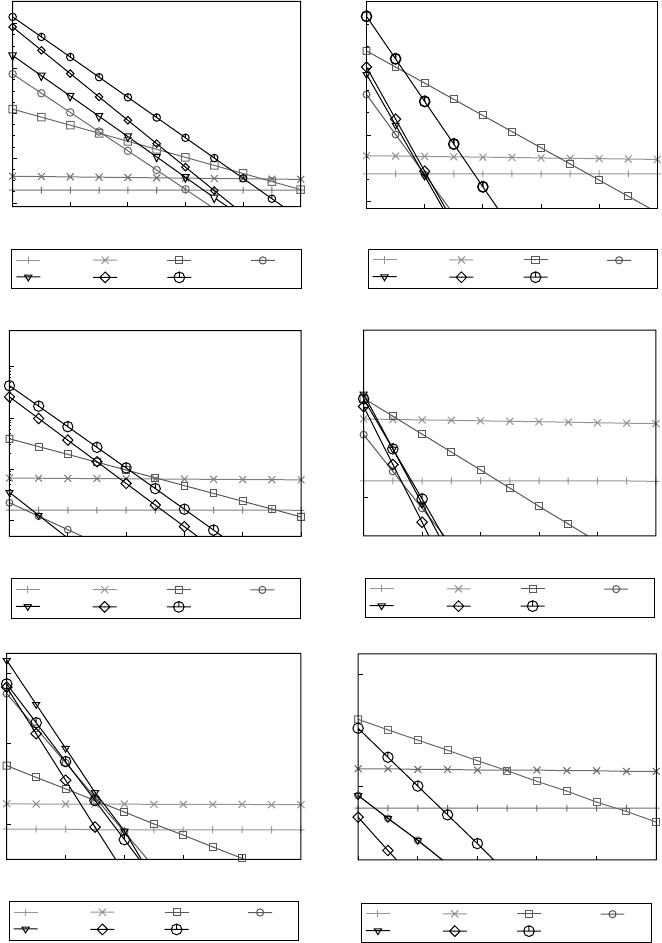
Figure 13.10 Parameter sensitivity of OLMAR-2 with respect to α with fixed ( = 10):
(a) NYSE (O); (b) NYSE (N); (c) TSE; (d) SP500; (e) MSCI; and (f) DJIA.
First, the transaction cost is an important and unavoidable issue that should be
addressed in practice. To test the effects of transaction cost on the proposed strategies,
we adopt the proportional transaction cost model stated in Section 2.2. Figure 13.11
depicts the effects of proportional transaction cost when the algorithms are applied
on the six datasets, where the transaction cost rate γ varies from 0% to 1%. We
present only the results achieved by three representative algorithms (CORN, PAMR,
T&F Cat #K23731 — K23731_C013 — page 118 — 9/28/2015 — 21:35
EXPERIMENT 4 119
10
0
10
4
10
8
10
12
10
16
0 0.2 0.4 0.6 0.8 1
Total wealth achieved
Transaction costs (γ%)
(a)
Β
ΝΝ
Market
CORN
BCRP
PAMR
Anticor
OLMAR
10
9
10
6
10
3
10
0
0 0.2 0.4 0.6 0.8 1
Total wealth achieved
Transaction costs (γ%)
(b)
Β
ΝΝ
Market
CORN
BCRP
PAMR
Anticor
OLMAR
10
3
10
2
10
1
10
0
0 0.2 0.4 0.6 0.8 1
Total wealth achieved
Transaction costs (γ%)
(c)
Β
ΝΝ
Market
CORN
BCRP
PAMR
Anticor
OLMAR
1
5
20
0
0.2 0.4
(d)
0.6 0.8 1
Total wealth achieved
Transaction costs (γ%)
Β
ΝΝ
Market
CORN
BCRP
PAMR
Anticor
OLMAR
1
5
20
0 0.2 0.4 0.6 0.8 1
Total wealth achieved
Transaction costs (γ%)
(e)
Β
ΝΝ
Market
CORN
BCRP
PAMR
Anticor
OLMAR
1
2
4
0 0.2 0.4
(f)
0.6 0.8 1
Total wealth achieved
Transaction costs (γ%)
Β
ΝΝ
Market
CORN
BCRP
PAMR
Anticor
OLMAR
Figure 13.11 Scalability of the proposed strategies with respect to the transaction cost rate (γ):
(a) NYSE (O); (b) NYSE (N); (c) TSE; (d) SP500; (e) MSCI; and (f) DJIA.
T&F Cat #K23731 — K23731_C013 — page 119 — 9/28/2015 — 21:35
120 EMPIRICAL RESULTS
and OLMAR) and ignore the results of CWMR, whose curves often overlap that
of PAMR. For comparison, we also plot the results achieved by two state-of-the-art
strategies (Anticor and B
NN
) and two benchmarks (BCRP and Market). Since most
follow the winner approaches try to approach BCRP, we ignore their figures.
From the figures, we can observe that the proposed algorithms can withstand
reasonable transaction cost rates, on most datasets. For example, the break-even rates
with respect to the market index vary from 0.2% to 0.8%, except DJIA, on which only
OLMAR can withstand around 0.3%. As CORN and PAMR/CWMR fail to beat the
markets on the DJIA dataset without transaction costs, their failures with transaction
costs can be naturally expected. On the other hand, the behaviors of the proposed
algorithms diverge. With a similar pattern-matching principle, CORN often performs
similar to B
NN
, while both of them generally underperform the mean reversion algo-
rithms. Since the three mean reversion algorithms (PAMR, CWMR, and OLMAR)
revert to the mean more actively than Anticor and thus result in more drastic portfolio
rebalances, they surpass Anticor with low or medium transaction costs and underper-
form Anticor with high transaction costs. Note that the transaction cost rate in the
real market is low
∗
; thus, the results clearly indicate the practical applicability of the
proposed strategies even when we consider reasonable transaction costs.
Second, margin buying is another practical concern for a real-world portfo-
lio selection task. To evaluate the impact of margin buying, we adopt the model
described in Section 2.2 and present the cumulative wealth achieved by the com-
peting approaches with or without margin buying in Table 13.3. The results clearly
show that if margin buying is allowed, the profitability of the proposed algorithms
on most datasets increases. Similar to the results without margin buying, certain pro-
posed algorithms often achieve the best results with margin buying. In summary, the
proposed strategies can be extended to handle the margin-buying issue and benefit
from it, and thus are practically applicable.
13.5 Experiment 5: Evaluation of Computational Time
Our next experiment is to evaluate the computational time costs of different
approaches, which is also an important issue in developing a practical trading strategy.
As previously analyzed, CORN has a batch-learning step on each period and is time
consuming in both its sample selection step and portfolio optimization step,
†
while
PAMR, CWMR, and OLMAR are online learning algorithms and cost linear time
per iteration. Table 13.4 presents the computational time cost (in seconds) of three
performance-comparable approaches (Anticor, B
K
, and B
NN
) on the six datasets. All
the experiments were conducted on an Intel Core 2 Quad 2.66 GHz processor with
4 GB RAM, using MATLAB
2009b on Windows XP.
‡
∗
For example, without considering taxesand bid–ask, Interactive Broker(www.interactivebrokers.com)
charges $0.005 per share. Since the average price of Dow Jones Composites is around $50.00 (as of June
2011), the transaction cost rate is about 0.01%.
†
In its MATLAB implementation, the latter step costs more than 80% of the total time.
‡
We use MATLAB function tic/toc to measure the time. There are preprocessing (such as data loader,
variable initialization, etc.) and postprocessing (such as result analysis, etc.), whose time is all excluded
from the time statistics in Table 13.4.
T&F Cat #K23731 — K23731_C013 — page 120 — 9/28/2015 — 21:35

EXPERIMENT 5 121
Table 13.3 Cumulative wealth achieved by various strategies on the six datasets without and
with margin loans (MLs)
NYSE (O) NYSE (N) TSE
Algorithms No ML With ML No ML With ML No ML With ML
Market 14.50 15.75 18.06 17.68 1.61 1.71
Best-stock 54.14 54.14 83.51 173.18 6.28 10.53
BCRP 250.6 3755.09 120.32 893.63 6.78 21.23
UP 27.41 62.99 31.49 57.03 1.60 1.69
EG 27.09 63.28 31.00 55.55 1.59 1.68
ONS 109.19 517.21 21.59 228.37 1.62 0.88
Anticor 2.41E+08 1.05E+15 6.21E+06 5.41E+09 39.36 18.69
B
K
1.08E+09 6.29E+15 4.64E+03 3.72E+06 1.62 1.53
B
NN
3.35E+11 3.17E+20 6.80E+04 5.58E+07 2.27 2.17
CORN 1.48E+13 6.59E+25 5.37E+05 7.31E+07 3.56 5.00
PAMR 5.14+15 5.57E+25 1.25E+06 1.12E+09 264.86 720.42
CWMR 6.49E+15 6.59E+25 1.41E+06 7.31E+07 332.62 172.36
OLMAR 3.68E+16 5.67E+30 2.54E+08 1.73E+12 424.80 31.63
SP500 MSCI DJIA
Algorithms No ML With ML No ML With ML No ML With ML
Market 1.34 1.03 0.91 0.69 0.76 0.59
Best-stock 3.78 3.78 1.50 1.50 1.19 1.19
BCRP 4.07 6.48 1.51 1.54 1.24 1.24
UP 1.62 1.75 0.92 0.71 0.81 0.66
EG 1.63 1.70 0.93 0.72 0.81 0.65
ONS 3.34 7.76 0.86 0.33 1.53 2.21
Anticor 5.89 10.73 3.22 3.40 2.29 2.89
B
K
2.24 1.88 2.64 6.56 0.68 0.56
B
NN
3.07 3.29 14.47 150.49 0.88 0.67
CORN 6.35 14.59 26.10 835.08 0.84 0.55
PAMR 5.09 15.91 15.23 68.83 0.68 0.84
CWMR 5.90 23.50 17.28 76.29 0.68 0.88
OLMAR 5.83 5.60 16.39 57.79 2.12 1.46
From the results, we can clearly see that CORN and the state-of-the-art algorithms
have high costs, and in all cases the proposed PAMR, CWMR, and OLMAR take
significantly less computational time than others. Even though the computational
time in daily back-tests, especially per trading day, is small, it is important in certain
scenarios such as high-frequency trading (Aldridge 2010), where transactions may
occur in fractions of a second. Nevertheless, the results obviously demonstrate the
computational efficiency of three proposed mean reversion strategies, which further
enhances their real-world large-scale applicability.
T&F Cat #K23731 — K23731_C013 — page 121 — 9/28/2015 — 21:35

122 EMPIRICAL RESULTS
Table 13.4 Computational time cost (in seconds) on the six real datasets
Algorithms NYSE (O) NYSE (N) TSE SP500 MSCI DJIA
Anticor 2.57E+03 1.93E+03 2.15E+03 387 306 175
B
K
7.89E+04 5.78E+04 6.35E+03 1.95E+03 2.60E+03 802
B
NN
4.93E+04 3.39E+04 1.32E+03 2.91E+03 2.55E+03 1.28E+03
CORN 8.78E+03 1.03E+04 1.59E+03 563 444 172
PAMR 8 7 2 1.1 1.0 0.3
CWMR 12 11 3 1.4 1.3 0.5
OLMAR 4 3 0.7 0.6 0.5 0.3
13.6 Experiment 6: Descriptive Analysis of Assets and Portfolios
Existing experiments on related studies (refer to Experiments 1 to 5) focus on com-
paring different algorithms based on various preceding aspects. In this section, we
perform a preliminary analysis of the behaviors of asset returns and portfolios, which
may reflect some insights into future study. While the analysis on different datasets is
similar, we focus on the standard benchmark dataset, NYSE (O) (Cover 1991).
∗
We
also append the data statistics and top five average allocations of our strategies and
the state-of-the-art algorithms on other datasets,
†
such as Appendix C.
Before analyzing their portfolios, we list some descriptive statistics on NYSE (O),
including each asset’s cumulative return over the whole periods, their (arithmetic)
return mean and standard deviation, and their autocorrelation with lag 1, in Table 13.5.
Then, we plot some representative approaches’ mean weights and standard devi-
ations in Figure 13.12, and list the top five average weights in Table 13.6. First, let
us analyze the BCRP strategy, whose portfolio has the same weights for every period
and thus has zero standard deviation. BCRP is essentially different from the best stock
strategy (asset #30), as the weight on the stock is zero. Interestingly, BCRP focuses
on the five most volatile stocks (refer to the highest Std values in Table 13.5), which
means that the portfolio selections are undiversified and verifies the “volatility pump-
ing” (Luenberger 1998) nature. Even though asset #23 does not perform as good as
most assets, its high volatility makes it the second weighted asset. This shows that
exploiting volatile stocks, even though some of them may perform poorly, can give
good performance.
For both EG and ONS, their portfolios have much lower volatility than other
strategies. In particular, EG’s portfolios always slightly drift around the initial uni-
form portfolio (for NYSE (O),
1
36
1). Such a phenomenon can be explained by its
learning rate (λ > 0), which has to be small such that the algorithm is universal.
However, decreasing the learning rate (λ → 0) ultimately approaches the algorithm
to uniform CRP.
‡
Our observation on EG’s portfolios verifies the previous analysis
on its parameter, in Section 4.2.
∗
Due to the table constraints, we use indices to represent individual assets, whose symbols are available
at http://stevenhoi.org/olps
†
We ignore TSE, which has too much assets (m =88) to show.
‡
Uniform CRP will be constant at uniform portfolio. This is approachable but not achievable as λ > 0.
T&F Cat #K23731 — K23731_C013 — page 122 — 9/28/2015 — 21:35
..................Content has been hidden....................
You can't read the all page of ebook, please click here login for view all page.