
![]()
This chapter discusses hash indexes, the new type of indexes introduced in the In-Memory OLTP Engine. It will show their internal structure and explain how SQL Server works with them. You will learn about the most critical property of hash indexes, bucket_count, which defines the number of hash buckets in the index hash array. You will see how incorrect bucket count estimations affect system performance. Finally, this chapter talks about the SARGability of hash indexes and statistics on memory-optimized tables.
Hashing Overview
Hashing is a widely-known concept in Computer Science that performs the transformation of the data into short fixed-length values. Hashing is often used in scenarios when you need to optimize point-lookup operations that search within the set of large strings or binary data using equality predicate(s). Hashing significantly reduces an index key size, making them compact, which, in turn, improves the performance of lookup operations.
A properly defined hashing algorithm, often called a hash function, provides relatively random hash distribution. A hash function is always deterministic, which means that the same input always generates the same hash value. However, a hash function does not guarantee uniqueness, and different input values can generate the same hashes. That situation is called collision and the chance of it greatly depends on the quality of the hash algorithm and the range of allowed hash keys. For example, a hash function that generates a 2-byte hash has a significantly higher chance of collision compared to a function that generates a 4-byte hash.
Hash tables, often called hash maps, are the data structures that store hash keys, mapping them to the original data. The hash keys are assigned to buckets, in which original data can be found. Ideally, each unique hash key is stored in the individual bucket; however, when the number of buckets in the table is not big enough, it is entirely possible that multiple unique hash keys would be placed into the same bucket. Such situation is also often referenced as a hash collision in context of hash tables.
![]() Tip The HASHBYTES function allows you to generate hashes in T-SQL using one of the industry standard algorithms such as MD5, SHA2_512, and a few others. However, the output of the HASHBYTES function is not ideal for point-lookup optimization due to the large size of the output. You can use a CHECKSUM function that generates a 4-byte hash instead.
Tip The HASHBYTES function allows you to generate hashes in T-SQL using one of the industry standard algorithms such as MD5, SHA2_512, and a few others. However, the output of the HASHBYTES function is not ideal for point-lookup optimization due to the large size of the output. You can use a CHECKSUM function that generates a 4-byte hash instead.
You can index the hash generated by the CHECKSUM function and use it as the replacement for the indexes on uniqueidentifier columns. It is also useful when you need to perform point-lookup operations on the large (>900 bytes) strings or binary data, which cannot be indexed. I discussed this scenario in Chapter 6 of my book Pro SQL Server Internals.
Much Ado About Bucket Count
In the In-Memory OLTP Engine, hash indexes are, in a nutshell, hash tables with buckets implemented as array of a predefined size. Each bucket contains a pointer to a data row. SQL Server applies a hash function to the index key values, and the result of the function determines to which bucket a row belongs. All rows that have the same hash value and belong to the same bucket are linked together through a chain of index pointers in the data rows.
Figure 4-1 illustrates an example of a memory-optimized table with two hash indexes defined. You saw this diagram in the previous chapter; it’s displayed here for reference purposes. Remember that in this example we assumed that a hash function generates a hash value based on the first letter of the string. Obviously, a real hash function used in In-Memory OLTP is much more random and does not use character-based hashes.

Figure 4-1. A memory-optimized table with two hash indexes
The number of buckets is the critical element in hash index performance. An efficient hash function allows you to avoid most collisions during hash key generation; however, you will have collisions in the hash table when the number of buckets is not big enough, and SQL Server has to store different hashes together in the same buckets. Those collisions lead to longer row chains, which requires SQL Server to scan more rows during the query processing.
Bucket Count and Performance
Let’s consider a hash function that generates a hash based on the first two letters of the string and can return 26 * 26 = 676 different hash keys. This is a purely hypothetical example, which I am using just for illustration purposes.
Assuming that the hash table can accommodate all 676 different hash buckets and you have the data shown in Figure 4-2, you will need to traverse at most two rows in the chain when you run a query that looks for a specific value.

Figure 4-2. Hash table lookup: 676 buckets
The dotted arrows in Figure 4-2 illustrate the steps needed to look up the rows for Ann. The process requires you to traverse two rows after you find the right hash bucket in the table.
However, the situation changes if your hash table does not have enough buckets to separate unique hash keys from each other. Figure 4-3 illustrates the situation when a hash table has only 26 buckets and each of them stores multiple different hash keys. Now the same lookup of the Ann row requires you to traverse the chain of nine rows total.

Figure 4-3. Hash table lookup: 26 buckets
The same principle applies to the hash indexes where choosing an incorrect number of buckets can lead to serious performance issues.
Let’s create two non-durable memory-optimized tables, and populate them with 1,000,000 rows each, as shown in Listing 4-1. Both tables have exactly the same schema with a primary key constraint defined as the hash index. The number of buckets in the index is controlled by the bucket_count property. Internally, however, SQL Server rounds the provided value to the next power of two, so the HashIndex_HighBucketCount table would have 1,048,576 buckets in the index and the HashIndex_LowBucketCount table would have 1,024 buckets.
Table 4-1 shows the execution time of the INSERT statements in my test environment. As you can see, inserting data into the HashIndex_HighBucketCount table is about 27 times faster compared to the HashIndex_LowBucketCount counterpart.
Table 4-1. Execution Time of INSERT Statements
dbo.HashIndex_HighBucketCount (1,048,576 buckets) | dbo.HashIndex_LowBucketCount (1024 buckets) |
|---|---|
3,578 ms | 99,312 ms |
Listing 4-2 shows the query that returns the bucket count and row chains information using the sys.dm_db_xtp_hash_index_stats view. Keep in mind that this view scans the entire table, which is time consuming when the tables are large.
Figure 4-4 shows the output of the query. As you can see, the HashIndex_HighBucketCount table has on average one row in the row chains, while the HashIndex_LowBucketCount table has almost a thousand rows per chain. It is worth noting that even though the hash function used by In-Memory OLTP provides relatively good random data distribution, some level of hash collision is still present.

Figure 4-4. sys.dm_db_xtp_hash_index_stats output
The incorrect bucket count estimation and long row chains can significantly affect performance of both reader and writer queries. You have already seen the performance impact for the insert operation. Now let’s look at a select query.
Listing 4-3 shows the code that triggers 65,536 Index Seek operations in each memory-optimized table. I wrote this query in very inefficient way just to be able to demonstrate the impact of the long row chains.
You can confirm that the queries traversed the row chains 65,536 times by analyzing the execution plan shown in Figure 4-5.

Figure 4-5. Execution plan of the queries
Table 4-2 shows the queries’ execution time in my environment where the query against HashIndex_LowBucketCount table was about 20 times slower.
Table 4-2. Execution Time of SELECT Statements
dbo.HashIndex_HighBucketCount (1,048,576 buckets) | dbo.HashIndex_LowBucketCount (1024 buckets) |
|---|---|
644 ms | 13,524 ms |
While you can clearly see that underestimation of the bucket counts can degrade system performance, overestimation is not good either. First, every bucket uses 8 bytes to store the memory pointer, and a large number of unused buckets is a waste of precious system memory. For example, defining the index with bucket_count=100000000 will introduce 134,217,728 buckets, which will require 128MB of RAM. This does not seem much in the scope of the single index; however, it could become an issue as the number of indexes grows up.
Moreover, SQL Server needs to scan all buckets in the index when it performs an Index Scan operation, and extra buckets add some overhead to the process. Listing 4-4 shows the queries that demonstrate such an overhead.
Table 4-3 shows the execution time in my environment. As you see, the overhead of scanning extra buckets is not significant; however, it still exists.
Table 4-3. Execution Time of SELECT Statements
dbo.HashIndex_HighBucketCount (1,048,576 buckets) | dbo.HashIndex_LowBucketCount (1024 buckets) |
|---|---|
313 ms | 280 ms |
Choosing the Right Bucket Count
Choosing the right number of buckets in a hash index is a tricky but very important subject. To make matters worse, you have to make the right decision at the design stage; it is impossible to alter the index and change the bucket_count once a table is created.
In ideal situation, you should have the number of buckets that would exceed cardinality (number of unique keys) of the index. Obviously, you should take future system growth and projected workload changes into consideration. It is not a good idea to create an index based on the current data cardinality if you expect the system to handle much more data in the future.
![]() Note Microsoft suggests setting the bucket_count to be between one and two times the number of distinct values in the index. You can read more at https://msdn.microsoft.com/en-us/library/dn494956.aspx.
Note Microsoft suggests setting the bucket_count to be between one and two times the number of distinct values in the index. You can read more at https://msdn.microsoft.com/en-us/library/dn494956.aspx.
Low-cardinality columns with a large number of duplicated values are usually bad candidates for hash indexes. The same data values generate the same hash and, therefore, rows will be linked to long row chains. Obviously, there are always exceptions, and you should analyze the queries and workload in your system, taking into consideration the data modification overhead introduced by the long row chains.
In existing indexes, you can analyze the output of the sys.dm_db_xpt_hash_index_stats view to determine if the number of buckets in the index is sufficient. If the number of empty buckets is less than 10 percent of the total number of buckets in the index, the bucket count is likely to be too low. Ideally, at least 33 percent of the buckets in the index should be empty.
With all that being said, it is often better to err on the side of caution and overestimate rather than underestimate the number. Even though overestimation impacts the performance of the Index Scan, this impact is much lower compared to the one introduced by long row chains. Obviously, you need to remember that every bucket uses 8 bytes of memory whether it is empty or not.
Changing the Bucket Count in the Index
As you already know, it is impossible to alter the table and change the bucket_count in the index after the table is created. The only option of changing it is to recreate the table, which is impossible to do while keeping the table online.
To make matter worse, the sp_rename stored procedure does not work with memory-optimized tables. It is impossible to create a new memory-optimized table with the desired structure, dump data there, and drop an old table and rename a new table afterwards. You will need to recreate an old table and copy data the second time if you want to keep the table name intact.
![]() Tip You can use synonyms referencing the new table under the old table name, making it transparent to the code. You can read more about synonyms at https://msdn.microsoft.com/en-us/library/ms187552.aspx.
Tip You can use synonyms referencing the new table under the old table name, making it transparent to the code. You can read more about synonyms at https://msdn.microsoft.com/en-us/library/ms187552.aspx.
When you want to keep the table name intact, you can export data to and import data from the flat files using the bcp utility. Alternatively, you can create and use either an on-disk or memory-optimized table as a temporary staging place.
Obviously, a memory-optimized table is the faster choice compared to an on-disk table; however, you should consider memory requirements during the process. Even though the garbage collector eventually deallocates deleted rows from the memory, it would not happen instantly after you dropped the table. You should have enough memory to accommodate at least two extra copies of the data to be on the safe side.
Do not create any unnecessary indexes on the staging table. Use heaps in the case of an on-disk table or a single primary key constraint with a memory-optimized table. This will help you to reduce memory consumption and speed up the process.
Finally, avoid using non-durable memory-optimized tables to stage the data. Even though this could significantly speed up the process and reduce transaction log overhead, you can lose the data if an unexpected crash or failover occurred during the data movement.
![]() Tip You can reduce transaction log overhead by staging data in another database temporarily created for such a purpose. You will still write the data to transaction log in the staging database; however, those log records won’t need to be backed up or transmitted over the network to the secondary servers. It is also beneficial to use the SELECT INTO operator when copying data into an on-disk table to make the operation minimally logged.
Tip You can reduce transaction log overhead by staging data in another database temporarily created for such a purpose. You will still write the data to transaction log in the staging database; however, those log records won’t need to be backed up or transmitted over the network to the secondary servers. It is also beneficial to use the SELECT INTO operator when copying data into an on-disk table to make the operation minimally logged.
Hash Indexes and SARGability
In the database world, queries are treated as SARGable (Search ARGument Able) when they and their predicates allow the Database Engine to utilize Index Seek operations during query execution.
Hash indexes have different SARGability rules as compared to B-Tree indexes defined on on-disk tables. They are efficient only in the case of a point-lookup equality search, which allows SQL Server to calculate the corresponding hash value of the index key(s) and find a bucket that references the desired chain of rows.
In the case of composite hash indexes, SQL Server calculates the hash value for the combined value of all key columns. A hash value calculated on a subset of the key columns would be different and, therefore, a query should have equality predicates on all key columns for the index to be useful.
This behavior is different from indexes on on-disk tables. Consider the situation where you want to define an index on (LastName, FirstName) columns. In the case of on-disk tables, that index can be used for an Index Seek operation, regardless of whether the predicate on the FirstName column is specified in the where clause of a query. Alternatively, a composite hash index on a memory-optimized table requires queries to have equality predicates on both LastName and FirstName in order to calculate a hash value that allows for choosing the right hash bucket in the index.
Let’s create on-disk and memory-optimized tables with composite indexes on the (LastName, FirstName) columns, populating them with the same data as shown in Listing 4-5.
For the first test, let’s run select statements against both tables, specifying both LastName and FirstName as predicates in the queries, as shown in Listing 4-6.
As you can see in Figure 4-6, SQL Server is able to use an Index Seek operation in both cases.

Figure 4-6. Composite hash index: execution plans when queries use both index columns as predicates
In the next step, let’s check what happens if you remove the filter by FirstName from the queries. The code is shown in Listing 4-7.
In the case of the on-disk index, SQL Server is still able to utilize an Index Seek operation. This is not the case for the composite hash index defined on the memory-optimized table. You can see the execution plans for the queries in Figure 4-7.

Figure 4-7. Composite hash index: execution plans when queries use the leftmost index column only
Statistics on Memory-Optimized Tables
Even though SQL Server creates index- and column-level statistics on memory-optimized tables, it does not update the statistics automatically. This behavior leads to a very interesting situation: indexes on memory-optimized tables are created with the tables and, therefore, the statistics are created at the time when the tables are empty and are never updated automatically afterwards.
You can validate it by running the DBCC SHOW_STATISTICS statement shown in Listing 4-8.
The output shown in Figure 4-8 illustrates that the statistics is empty.

Figure 4-8. Output of DBCC SHOW_STATISTICS statement
You need to keep this behavior in mind while designing a statistics maintenance strategy in the system. You should update the statistics after the data is loaded into the table when SQL Server or the database restarts. Moreover, if the data in a memory-optimized table is volatile, which is usually the case, you should manually update statistics on a regular basis.
You can update individual statistics with the UPDATE STATISTICS command. Alternatively, you can use the sp_updatestats stored procedure to update all statistics in the database. The sp_updatestats stored procedure always updates all statistics on memory-optimized tables, which is different from how it works for on-disk tables, where such a stored procedure skips statistics that do not need to be updated.
SQL Server always performs a full scan while updating statistics on memory-optimized tables. This behavior is also different from on-disk tables, whereas SQL Server samples the data by default. Finally, you need to specify the NORECOMPUTE option when you run CREATE STATISTICS or UPDATE STATISTICS statements. Listing 4-9 shows an example.
If you run the DBCC SHOW_STATISTICS statement from Listing 4-8 again, you should see that the statistics have been updated (see Figure 4-9).

Figure 4-9. Output of DBCC SHOW_STATISTICS statement after the statistics are updated
Missing statistics can introduce suboptimal execution plans with the nested loop joins when SQL Server chooses inner and outer inputs for the operator. As you know, the nested loop join algorithm processes the inner input for every row from the outer input, and it is more efficient to put smaller input to the outer side. Listing 4-10 shows the algorithm for the inner nested loop join as the reference.
Missing statistics can lead to a situation when SQL Server choses the inner and outer inputs incorrectly, which can lead to highly inefficient plans.
Let’s create two tables, populating them with some data, as shown in Listing 4-11.
The data in both tables distributed unevenly. You can confirm it by running the query in Listing 4-12. Figure 4-10 illustrates the data distribution in the tables.

Figure 4-10. Missing statistics and inefficient execution plans: data distribution
As the next step, let’s run two queries that join the data from the tables as it is shown in Listing 4-13. Both queries will return just a single row.
As you can see in Figure 4-11, SQL Server generated identical execution plans for both queries using the T1 table in the outer part of the join. This plan is very efficient for the first query; there is the only one row with T1Col = 2 and, therefore, SQL Server had to perform an inner input lookup just once. Unfortunately, it is not the case for the second query, which leads to 4,095 Index Seek operations on the T2 table.

Figure 4-11. Missing statistics and inefficient execution plans: execution plans
Let’s update statistics on both tables, as shown in Listing 4-14.
Figure 4-12 illustrates that the statistics have been updated.
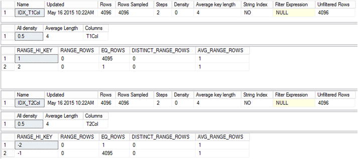
Figure 4-12. Missing statistics and inefficient execution plans: index statistics
Now, if you run the queries from Listing 4-13 again, SQL Server can generate an efficient execution plan for the second query, as shown in Figure 4-13.

Figure 4-13. Missing statistics and inefficient execution plans: execution plans after statistics update
![]() Note You can read more about statistics on memory-optimized tables at http://msdn.microsoft.com/en-us/library/dn232522.aspx.
Note You can read more about statistics on memory-optimized tables at http://msdn.microsoft.com/en-us/library/dn232522.aspx.
Summary
Hash indexes consist of an array of hash buckets, each of which stores the pointer to the chain of rows with the same index key column(s) hash. Hash indexes help to optimize point-lookup operations when queries search for the rows using equality predicates. In case of composite hash indexes, the query should have equality predicates on all key columns for the index to be useful.
Choosing the right bucket count is extremely important. Underestimations lead to long row chains, which could seriously degrade performance of the queries. Overestimations increase memory consumption and decrease performance of the index scans.
Low-cardinality columns lead to the long row chains and are usually bad candidates for hash indexes.
You should analyze index cardinality and consider future system growth when choosing the right bucket count. Ideally, you should have at least 33 percent of buckets empty. You can get information about buckets and row chains with the sys.dm_db_xtp_hash_index_stats view.
SQL Server creates statistics on the indexes on memory-optimized tables; however, statistics are not updated automatically. You should update statistics manually using the UPDATE STATISTICS statement or the sp_updatestats procedure on a regular basis.