Technology and Invention: A Combinatorial Process

Ray Kurzweil, the noted inventor and futurist, once said that the exponential growth curves exhibited by current technological trends is based on the tendency of technology to ‘feed off’ technology. In light of the pace of change that we currently witness, this can be accepted as a fair statement if we are to accept that every technology that has been invented, is being invented and will be invented follows the very same formula - they are combinations of technologies that already existed and do not come out of sheer inspiration alone.

This might seem like a common-sense statement to some and in the past, philosophers, historians, sociologists and economists, such as Lewis Mumford, George Basalla, Joel Mokyr and Paul Romer, have come up with anecdotal theories that state this as a concept. But if we are to respect the Popperian scientific method to making a claim, then we need to consult the research that pertains to this subject to prove our hypothesis. More importantly, if we are to state that technology is created by combining bits and pieces of previous technological inventions, then we also need to extend this hypothesis to the process of invention as it is invention that generates new technologies.

Studies done by researchers from the Santa Fe Institute and the Oxford Martin School have found that invention, and thus almost any technology by proxy, exhibits this combinatory phenomenon. In a 2015 paper published by the Royal Society,¹ titled, ‘Invention as a combinatorial process: evidence from US patents’, the researchers studied US patent records from 1790 to 2010 in an attempt to conceptualize invention, which is how we get new technologies. Patents were considered as the ‘carriers’ of technology or as the ‘footprints’ of invention, as they leave behind a documentary trail in the way technologies evolve. By executing this study, the researchers were able to show that invention was the manner in which technologies (either very new or previously in use), were brought together and combined in ways not previously seen (Youn et.al, 2015). As per this study, and others² that have begun investigating the concept of combinatorial evolution ³ of technology, invention can be conceptualised as combinatorial possibilities. In other words, invention is simply the novel combination of existing technological capabilities and is evolutionary⁴ in nature.

This tendency of technology to build itself on previous or existing technologies is very similar to biological evolution. Kevin Kelly makes the analogy between biological evolution and technological evolution in a more succinct manner. As per his research, the long-term co-evolutionary trends seen in natural and technological paradigms share five common salient features: Specialisation, Diversity, Ubiquity, Socialization and Complexity. These five features are exhibited by any technology. As FinTech is one of the protagonists in this book and in modern capitalism, let’s analyse the evolution of this technology:

Financial technology finds its roots in the history of computing (refer Notes: A brief history of computing). Initially computers were made for very specific or specialised operations . For example, early computers such as the Differential Analyser, invented by Vannevar Bush in the mid 1930’s, were analog computation machines⁵ that were created to solve ordinary differential equations to help calculate the trajectories of shells. As World War Two broke out, these advances in computing were adopted and developed by various militaries to communicate sensitive information by integrating the techniques of cryptography - a kind of natural selection. To combat this, pioneers such as Alan Turing and his mentor Max Newman, set about designing and building automated machines (Turing Machines) that could decrypt these camouflaged communiqués. This effectively changed the use of the computer and increased the diversity of the kinds of computers.

After the war, advances by notable inventors such as John Mauchly, Presper Eckert and John von Neumann (a veritable polymath) led to the creation of the EDVAC (Electronic Discrete Variable Automatic Computer) , the first binary computer. With binary computers coming of age, there was an increasing need to develop software to give instructions to computers. Punch cards were soon replaced by logic gates (from Boolean algebra) and languages such as COBOL and FORTRAN (FORmula TRANslation), helped in the creation of early operating systems. As software design began to evolve so did the functionality of computers. Programming languages and such as BASIC, LISP, SIMULA, C, C++, UML, Unix, Linux, etc., helped in the construction of distributed communication networks, the internet and ultimately the worldwide web. As the cost of transistors began to drop (Moore’s Law), more tasks got computerized leading to the ubiquity of computers in almost all functions of business and life.

This ubiquitousness gradually entered the sector of trade and thus finance. As trade is a fundamental social interaction, the socializationof computers for communication and value exchange was a natural evolutionary technological development. Increased socialization via digital channels over the past two decades has led to more interconnections between different nodes and led to a complex interwoven structure, where there is no central point that holds the entire edifice in place. As the developmental process of computing continues to become increasingly distributed, the future of computing (and Fintech by extension), is bound to increase in complexity. Selection, diversity, incremental variation and temporal progression (Wagner & Rosen, 2014) will be the hallmarks of tomorrow’s technology and captialism.

It is the final stage of complexitythat poses the greatest intellectual challenge to our understanding of modern day capitalism. As the previous chapters have shown, the increased complexity that has arisen with the socialization and financialisation of banking and commerce has created a system that is opaque and difficult to regulate. The entry of new technologies in the financial system, such as the Blockchain, will help us gain more transparency but will also further add complexity to the system, as every participating node will become a point of both communication and value exchange. If regulators face difficulties identifying points of systemic risk and malicious players in an economy today, the problem is bound to get increasingly complicated in a more inclusive and complex cashless system.

Secondly, we also need to consider the accelerating consilience of technology. The concept of accelerating consilience of technology needs to be highlighted as it sets the stage for understanding the reason why there is a disconnect between the way economics and technology is studied and analysed. This disconnect is especially important as the pace of technological evolution and the disruptive impact it has on the economy is getting shorter and quicker as seen in Figure 4-1.

Figure 4-1. The quickening pace of Konratiev waves Source: The Economist, ‘Innovation in Industry - Catch the Wave’, 1999.⁶

As technology continues to accelerate, it has a profound impact on the economy as technological performance results in reduction of production costs. Wright’s law (1936) and Moore’s Law (1965) shows that as technological performance increases, it is accompanied with a reduction in the cost of production (Figure 4-2). Theodore Wright (who created Wright’s Law) predicted in 1936 that as technologies improve exponentially with time, costs would decrease as a power law of cumulative production. Some recent research from MIT and the Santa Fe institute shows that a combination of an exponential decrease in cost and an exponential increase in production would make Moore’s law and Wright’s law indistinguishable (as originally pointed out by Sahal) (Nagy et al., 2013).

Figure 4-2. Technology curves and their economic effect on the cost of production. Left image: Wright’s Law (1936); Right image: Moore’s Law (1965) Sources: Left image - Wikipedia; Right image - http://dx.doi.org/10.1371/journal.pone.0052669

This link between the combinatorial evolution of technology and the effect it has on a networked economy is key to understanding not just the economic impact of technological progress, but also in understanding a key tenet of modern day capitalism - technology and the economy follow the same patterns of evolution as seen in ecological systems, and in doing so, increase the complexity of the system.

The Blockchain (which itself is a combination of cryptography, computer science, game theory and monetary economics), is just one element that is increasing the complexity of economics. Other technologies, which have also been discussed in this book, show that most new businesses being created today do not depend on a single technology to propose value to clients. It is because of this accelerating consilience that new businesses are able to scale faster than in comparison to the path that was followed by older incumbents.

If the economy were to be looked at as a network of production agents where each node is an industry, then owing to the consilience of technology, the goods produced by one industry are used as inputs to another industry. As technology from one industry begins to combine with that of another, innovations occur which lead to production cost reductions and the emergence of new technologies. As the inputs get cheaper or better in terms of efficiency, it leads to the creation of new goods. As new products become ubiquitous, improved social connections (including management styles), lead to better distribution of the technology and the associated economies of scale. The greater the connection between the industries, i.e.: the more networked the structure of the economy, the faster this phenomenon repeats itself leading to exponential changes in technological evolution and production cost reductions (Also refer, Farmer and Lafond, 2015).

We can infer from the above statement, that technology and investment decisions are in a constant state of change and are rarely static. But while the endogenous role of technology in the economy has gained increased traction in academic circles, the study of economics has yet to make the transition towards treating change in the economy as an entropic system immersed in an ecological environment. Even one of the most highly cited papers on this subject, ‘Endogenous Technological Change’ (1990), by Paul M. Romer, the current Chief Economist of the World Bank, is modelled around finding the state of equilibrium in light of technological change.⁷

As these physical flows of technology are accompanied by monetary flows, the economic impact of technological change are two sides of the same coin. As technological complexity continues to increase, the networked economy of modern day capitalism is bound to get more complex as well. But in spite of this increasing complexity and the accompanying entropy that is tied to it, the economic models that are used today are still based on states of equilibrium.

Therefore, if we are to fix the disconnected views we have about technology and economics, we need to rethink economic theory. As a system gets more complex, new bonds are formed, old bonds are destroyed and the repercussions of these creative - destructive movements create a state of constant change or entropy. So why is it that when we learn about economics, we are taught theories of equilibrium and rational expectations , when the changes occurring are entropic and mostly unforeseen, i.e. not rationally expected? If technology creates complexity, why is that the theories of economics are based on states of equilibrium in spite of the fact that changing nature of technology is highly endogenous to economics and capitalism? A primary reason for this mode of thinking is based on how we cognitively interpret the world and why we are constantly trying to predict the future. Sidebar 4-1 offers some neuroscience insights.

Sidebar 4-1: A Rationale for Rational Expectations:

Sources: ‘How to Create a Mind: The Secret of Human Thought Revealed’, Ray Kurzweil (2014); ‘Neuroscience for Organizational Change’, Hilary Scarlett, (2016); ‘Social Cognitive Neuroscience of Leading Organizational Change’, Robert A. Snyder, (2016).

Rational Expectations is based on the innate working methodology of the human brain. We must remember that the human brain did not evolve in the current cosmopolitan and urban environment. It was designed in the treacherous environment of the Savannah thousands of years ago, and evolved to achieve two primary objectives: How to survive and how to predict.

Survival is the brain’s natural state and is based on a trade-off between Risk and Reward. As there were more risks in the early environments of humans, it was more important to identify risk to survive. As a result, the brain is more attuned to this state. When presented with any situation, the brain analyses any potential risks to survival and this primary instinct is faster to kick in, has stronger impulses and sensations and lasts longer as a memory. When certain stimuli trigger the reward network of the brain, studies show that the brain reacts slower (as it is not our natural state). The sensation is also milder and relatively short-lived (you forget praise after a few days, but not abuse).

To be able to survive in the face of constant risk, the brain had to be able to predict. In fact, the brain can be seen as a constant prediction machine that is continuously trying to find safety and avoid risk. Our brain’s neocortex constantly predicts what it expects to encounter. It is an ingenious tool that recognises, remembers and predicts patterns sans arrêt and develops hypothesises of what we will experience. As Ray Kurzweil puts it, predicting the future is actually the primary reason that we have a brain. The statement below exemplifies how the brain is constantly predicting, even when there is no sign of apparent danger:

“I cnduo’t bvleiee taht I culod aulaclty uesdtannrd waht I was rdnaieg. Unisg the icndeblire pweor of the hmuan mnid, aocdcrnig to rseecrah at Cmabrigde Uinervtisy, it dseno’t mttaer in waht oderr the lterets in a wrod are, the olny irpoamtnt tihng is taht the frsit and lsat ltteer be in the rhgit pclae. The rset can be a taotl mses and you can sitll raed it whoutit a pboerlm”.

But the exercise of prediction is a fatiguing one. The brain constitutes only 2% of our body mass but consumes 20% of our energy. As a result, the brain tries to save energy by taking cognitive shortcuts. It attempts to make predictions using abstract concepts and even if we are exposed to events with multidimensional aspects, the brain represents the pattern of events in a one-dimensional sequence of lower-level patterns. In other words, the innate built-in predictors of our brain try to save energy by thinking in terms of linearity. Our brains are most comfortable making predictions that possess a linear function.

Consider this simple example: a bat and ball cost €1.10. The bat costs €1 more than the ball. So how much does the ball cost? In most cases, the first answer that our minds instinctively predict is 10 cents. But if we were to work out this simple calculation, we would find that the actual cost of the ball is 5 cents. ((Bat + Ball = 1.10); As (Bat = 1+Ball); This means ((Bat + Ball) = (2 Ball + 1) = 1.10); Therefore, 2 Ball = 0.10; Ball = 0.05).

The historic tendency of the brain to prefer linear predictability could be why we have struggled in our modifying our method of economic thinking in the context of technological change. Both these subjects may have displayed linear growth trends in the past. But as we have discussed in the introduction to this chapter, technology is based on consilience the integration of older technologies.

As technology gets increasingly digitized, the consilience of technology is accelerating and evolving at an exponential rate. The logarithmic curve seen in Figure 4-3 is representative of this fact

Figure 4-3. Moore’s Law: Over 199 Years And Going Strong Image Source: BCA Research Special Report, ‘Human Intelligence and Economic Growth - From 50,000 B.C. to the Singularity’ (2013).

As the graph shows, these exponential curves are relatively recent in the history of economics. When Adam Smith published the ‘Wealth of Nations’, in 1776, the subject of economics represented linear scales. Technology evolved at a much slower pace (refer to Figure 4-1) and this made the social science of economics develop models that were well suited to linear technological growth curves and our linear way of predictive thinking. For a long time, this was the status quo and the Rational Expectations theory (RET) was not an error but a natural representation of simpler economies.

But as technology evolves and begins to grow at exponential rates, the increasing complexity that it is creating is challenging this theory. RET is based on the theory of perfect competition in economics which postulates perfect knowledge. But as interactions grow increasingly, the view the participants have of the economic system is always partial and distorted due to information asymmetries. So how can we ‘rationally’ expect anything when we do not have ‘perfect’ knowledge?

The information provided by the Blockchain will help us address this issue to a certain extent, as will new data analysis techniques . But the exercise of knowing everything about the economy seems like an asymptotic pursuit of perfection. It for this reason that when looking at the economy, we need to predict in terms of probability of the outcomes rather than creating exact linear models. The task of rethinking economics via this lens will be a daunting challenge, but remains feasible in my opinion. One of the most surprising results of recent research in neuroscience is the neuroplasticity (see notes) of the brain. The brain is constantly updating its cognitive map, or belief system, based on new information. As new ideas take hold, older beliefs are upgraded or discarded. Economics maybe an old discipline of study, but science shows us that we can still teach an old dog new tricks.

Economic Entropy versus Economic Equilibrium

Technology is generally studied as per the scientific method since science is the creative engine of technology. The scientific method was best described by the philosopher Karl Popper, who stated that any science should be scrutinized by decisive experimentation to determine a scientific law. As per this method, also known as Popperian falsifiability , the empirical truth of any scientific law cannot be verified beyond a shadow of a doubt and cannot be known with absolute certainty. They can only be falsified by testing - Even a single failed test is enough to falsify and no number of conforming instances is sufficient to verify. Scientific laws, and thus the study of technology, are hypothetical in character and their validity remains subject to testing.

While the scientific method largely applies to the natural sciences, its rigors ensure the establishment of facts. But while we hold the natural sciences to such exacting standards, we do not extend the same discipline of analysis to the social sciences, especially to economics. Indeed, for the past several decades, mainstream economics has been less concerned with describing reality and has preferred to base its theories on an idealised version of the world. The reason for this could possibly be traced backed to the neuroscience findings we have discussed in Sidebar 4-1. Conventional economics, after all, is searching for an answer to a difficult question that is very centric to human society - it wishes to know how agents in the economy (banks, firms, investors and consumers) might react to the general pattern of the economy they are creating together. Linear models that are easier to digest offer a delicious simplicity.

As a result, to answer this question, contemporary economics has preferred to dogmatically adhere to theories based on what it considers are reasonable axioms. The most eminent of these theories is the Efficient Market Hypothesis (EMH ) which sees the economy as a perfect, rational, mechanistic entity, where asset prices fully reflect all available information. Agents thus logically behave (perform actions, create strategies, make forecasts) in aggregate patterns that would represent all the information at their disposal. As a result, as per RET, all agents have a single optimum view of the future and over time all market participants converge around that view. If one agent were to execute an action that was contrary to this view, another agent would behave in a way to leverage that action to his or her interest and offset the discrepant action. The result is an economy that is static in origin and always trying to achieve equilibrium.

This theory of economics, although very eloquent, is quite absurd. It is completely divorced from actual data and any kind of scientific method. While EMH states that agents are ‘utility maximising’ and make decisions based on RET, almost no agent has the time nor the resources to go through the optimisation process and calculate the best course of action. Even if agents had all the information, the complexity of the decision-making process at hand (especially in light of the information overload provided by today’s technologies), means that computation of such a task is bound to be restricted to ‘good enough’ rather than the ‘best one under all circumstances’. Moreover, agents can make choices for moral or superstitious values that might have nothing to do with rationality. But neither the EMH, the RET or any mathematical framework of economics take these conditions into consideration. Not only are they devoid of good scientific practices, they are detached from human interests and societal reality.

Economics is a social science because it involves people and social interactions that are demonstrated in acts of trade and social allegiances. Although every participant is working towards his or her individual benefit, their view of the world is always incomplete and their actions are always biased. Owing to this, they will not take the appropriate action as stipulated by EMH and RET . George Soros defines this incomplete view of the world as the ‘principle of fallibility’ and the biased decision making process as the ‘principle of reflexivity’ in his ‘Theory of Reflexivity’.

Soros first published his theory of Reflexivity in his book, ‘The Alchemy of Finance’, in 1987. The book was a big success as fund managers and investors clamoured to discover what his investment secrets were. But very little attention was paid to his philosophy of Reflexivity. In a lecture⁸ he gave following the publication of his book, Soros himself said, “the philosophical arguments [in his book] did not make much of an impression. They were largely dismissed as the conceit of a man who has been successful in business and fancied himself as a philosopher”. However, the theory is interesting because of the principle role uncertainty plays in it.

Uncertainty is something that is normally reserved to risk assessment . EMH and RET do not stipulate exacting codes of conduct or modes of operation to encompass the concept of uncertainty. However, uncertainty needs to addressed at a fundamental level as the economic decisions made by agents bask in uncertainty. Agents making decisions (be it buying, selling, producing, strategizing, or forecasting), also have to anticipate the future decisions that other agents are going to make. Market prices, after all, are the agents weighted-average view of what is going to happen in the future. As the future is contingent on accurately anticipated decisions of others, uncertainty poses a central role in logical economic decision making.

RET circumvents this problem by postulating that in every market, there is a single optimal set of expectations and agent’s views will converge around it. But this hypothesis bears no resemblance to reality. In practice, every agent has different interests and since these interests cannot be known, agents have to make their decisions in conditions of uncertainty as there is no other choice. Their decisions are bound to be based on information asymmetries and personal biases. This is seen in the form of asset price distortions, fluctuating stock prices and currency volatility. Soros called this phenomenon of volatility and distortion owing to personal decision making the ‘ human uncertainty principle’.

The human uncertainty principle and the volatility that is brings along with it, are the fundamental reasons why the economy is never in a state of equilibrium. Individual decisions made by agent’s cause price distortions which set in motion boom-bust phenomena, leading to the creation of bubbles, crises and recessions. The past four decades have seen 8 major crises,⁹ or a crisis every five years on average. If there is anything that is constant in the economy, it the fact that it is in a constant state of entropy.

Thus, the first point to consider when deciding how to rethink the study of the economics is to acknowledge that agents in an economy react to the outcomes that have been created by others as well as themselves. As these decisions lead to volatility, an economy should not be looked at as a machine-like system operating at equilibrium, but more like an ecology where actions, strategies, and beliefs compete simultaneously creating new behaviours in the process. In other words, an economy is always forming and evolving, and not necessarily in equilibrium.

Secondly, we need to consider the relationship between technology and the economy , for while the economy creates technology, it is also created by technology, as has been explained earlier. The impact of technolgy on the economy has also been discussed in a number of recent works such as Brynjolfsson’s and McAfee’s Race Against the Machine (2011). The economy is therefore not just a container of technology but also an expression of them (Arthur, 2014). As technology changes, markets, regulations and policies need to change as well. In essence, technological change restructures the economy.

Owing to the constant change that is predicated by uncertain agent decisions and technological evolution, the economy is in fact usually in disequilibrium and behaves more like an organic entity in a vibrant ecology, where structures are constructed and reconstructed, and where openness to change is emphasised. Just as technology is endogenous to the economy, so is disequilibrium. Equilibrium could exist, but it is a temporary state of existence. Non-equilibrium is the natural state of affairs.

If the economy is seen in this light, then the reactions of technology with agents and the following assemblages and adaptations that are seen in an economy are reflective of the study of complex systems, an academic discipline that observes the deep laws of complexity and emergence in any system. Complexity theory was born in the 1970’s (Wilson, 1998) and was originally inspired by 19^th century physics, specifically the fields of classical mechanics, statistical non-equilibrium physics and thermodynamics (Helbing and Kirman, 2014). The main tenets of complexity theory borrow their conceptions from chaos theory, self-criticality and adaptive landscapes, to bring into focus the way complex systems grow, persist and collapse.

The first scholars of complexity theory began their formulations at the Santa Fe institute, and based their study of complex systems on abstract non-linear transformative computer simulations. They attempted to recreate the same phenomenon seen in complex systems, be it rain forests or collisions of protons in the large hadron collider (LHC ¹⁰), in massive computer-aided simulations. By adopting this approach, they attempted to achieve a higher level of understanding comprehensive systems consistent in the real world. In the past, this group of scientists were largely ignored by mainstream academia as traditional academics found their conclusions too vague and metaphoric.

This was partly due to two reasons - the lack of data and slow computing power provided insufficient evidence to support their theories. But over the past two decades this has changed. Increasing amounts of data and exponential rises in computing power, now allow practitioners of this discipline to recreate and study complex operations, such as, simulating the remnants left behind after proton bombardments. As the study of complexity gained traction, a few of the members of the Santa Fe institute began to ponder if the methods and tools at their disposal would allow them to study the interactions that were occurring in a complex economic system? A result of this thought experiment led to the creation of complexity economics in the early 1990’s.¹¹

Complexity economics does not attempt to sidestep the complexity and entropy of a dynamic, vibrant and ever changing economic ecosystem. On the contrary, the very basis of complexity economics is to use tools and methods that inculcate non-equilibrium phenomenon. The mathematics of complexity science is based on non-linearly interacting components (agents), where the system spends long periods of time far from equilibrium. The system may exhibit multiple states of equilibria, but these states are unstable and temporary as feedback and emergent properties (such as new technology), produce counter-intuitive behavioural traits. The system is studied as a highly connected network with no top-bottom control parameters, and where agents are unable to behave as they prefer since they cannot act independently.

All these features are observed in our current economic and financial markets, especially when considering the emergence and growing popularity of distributed value exchange networks. But in spite of this, owing to our dependence and attachment to out-dated dogmas of economic thought, we continue to delude ourselves in thinking that the economy functions in a state of equilibrium, and study the subject based on this convenient view.

It is surprising that this mode of thinking is the dominant view not only in academia, but also in economic governance. One might think that if commercial banks were investing millions of dollars in Blockchain technology, then policy makers would also be updating their methods and models of analysis according to the capabilities of the new systems. Would it not be sensible to prepare for a Blockchain future by developing tools and methods that are capable of leveraging the real-time transactional data between multiple economic agents who are making Knightian decisions¹² on a transparent cashless Blockchain? The answer of course, is no.

In spite of the similarities between complex economic systems and our current (and future) economic system, we continue to use models based on the general equilibrium economic theory, the most popular of which, is the Dynamic Stochastic General Equilibrium Model (DSGE ). DSGE based models have been dominant tools in macroeconomic modelling, economic forecasting and policy construction since the early 1980’s and continues to play this role today - For example, in 2009 the Reserve Bank of New Zealand developed and adopted the KITT (Kiwi Inflation Targeting Technology) DSGE model as their main forecasting and scenario tool (Beneš et al., 2009). Hence, to fully understand why we need to consider the use of complexity based models, in the context of the Blockchain, it is essential for us to first review equilibrium economic models.

The Mathematical Wizardry of Equilibrium Economic Models

Today, most central banks use DSGE models for monetary policy analysis and business cycle forecasting. As we have seen in Chapter 3, it is monetary and fiscal policy that play a determining role in guiding the state of markets and the prosperity of a nation. Thus, owing to their fundamental role in monetary policy decision making, it is important to understand the history, abilities and limitations of these models.

Currently, most central banks, such as the Federal Reserve and the ECB,¹³ use two kinds of models to study and build forecasts about the economy (Axtell and Farmer, 2015). The first, statistical models , fit current aggregate data of variables such as GDP, interest rates, and unemployment to empirical data in order to predict/suggest what the near future holds. The second type of models (which are more widely used), are known as “Dynamic Stochastic General Equilibrium” (DSGE) models . These models are constructed on the basis that the economy would be at rest (i.e.: static equilibrium) if it wasn’t being randomly perturbed by events from outside the economy.

Although DSGE models are dynamic macroeconomic models of business cycle behaviour, their foundations are derived from microeconomics as they assume that the economy is based on optimising agents who make decisions based on rational expectations to maximize their objectives based on constraints¹⁴ (Slobodyan and Wouters, 2012). The agents in the models are represented as households and firms - households consume goods, provide labour, invest and trade in bonds and accumulate capital in the form of real estate or liquidity. On the flipside, firms manufacture goods, provide employment and try to maximize profits based on their constraints. The interactions between firms and households result in guiding the economy through various stages of the business cycle and the central bank changes the nominal interest rate in response to changes in inflation, output, or other economic conditions. The central bank thus acts as a reactionary entity (in the context of the Taylor rule ¹⁵) in DSGE models. To account for fiscal shocks, the models contain some portion of ‘non-optimizing’ households which deplete all their earnings. In the language of political correctness, these households are referred to as hand-to- mouth households. Notice the emphasis on business cycles, assumptions and rational expectations.

The origins of these models can be traced back to the 1940’s, following the publication of Keynes’ General Theory (1936). Following the publication of this seminal work, governmental and academic bodies began the construction of large-scale macroeconomic models based on this style. Specific or ad-hoc rules were postulated, converted into variables and equations were created based on Keynesian macroeconomic theory . For close to three decades, these neo-Keynesian modelswere the mainstay of macroeconomic decision making.

But as the 1960’s ended and the 1970’s rolled in, advances in technology challenged the assumptions on which these models were built. As these models depended on a direct trade-off between inflation and unemployment, they were unable to appropriately consider the labour replacement function of technology. Secondly, they were incapable of integrating variables that represented microeconomic changes such as the elastic substitution of goods, the elasticity of labour supply (especially as technology replaced physical labour making economies more service oriented rather than manufacturing intensive), etc. Finally, they did not recognize that the decision-making rules of economic agents would vary systematically with changes in monetary policy. This final flaw is often referred to as the Lucas Critique.

The Lucas Critique and the introduction of Rational Expectations (following a seminal paper by Muth in 1961), led to demise of neo-Keynesian models. In its stead, DSGE models came into being. The first DSGE models were known as Real Business Cycle (RBC) modelswere introduced in the early 1980’s and were based on the concepts detailed by Finn E. Kydland and Edward C. Prescott in 1982. RBC models were based on the assumptions of perfect competition on the goods and labor markets and flexible prices and wages, and increasingly gained traction thanks to their success in matching some business cycle patterns (Slanicay, 2014). These models saw business cycle fluctuations as the efficient response to exogenous changes which implied that business cycles were created by ‘real’ forces and that productivity shocks were created by technological progress.

But in spite of the theoretical underpinning that technology was the main source of business fluctuations, after a period of use, the RBC model began to lose favour with academics and policy makers. A host of empirical studies found that the contribution of technology shocks to the business cycle fluctuations was relatively small and the predictions made by RBC models with regards to labour and productivity in response to technology shocks began to be rejected. A second reason for their rejection was their view on monetary policy - In most RBC models, monetary policy was taken to have no effect on real variables even in the short run. This was at odds with the longstanding belief of that monetary policy had the power to influence productivity output and unemployment in the short term (Christiano et al., 1998)(Also see ‘The Trouble With Macroeconomics’, Romer (2016) .

Owing to these differences, the RBC models began to undergo a phase of evolution which led to the creation of another class of DSGE models also known as New Keynesian models (NK models). These models were build on top of the existing framework of RBC models but their construction was also influenced by a new theory that had begun to gain increasing traction in the field of economics at that time - contract theory. This theory might be familiar to most readers, as two of the three¹⁶ economists who developed the theory received the Nobel Memorial Prize in Economic Sciences in October 2016.

Contract theory introduced the concepts of price and wage rigidities (See Sidebar 4-2 and ‘Theories of Wage Rigidity’, Stiglitz, 1984) in NK models . The older RBC models were thus enhanced with some Keynesian assumptions, namely competition on goods, labour and rigidities. By including nominal price and wage rigidities into the model, changes in short-term nominal interest rate were not offset by identical changes in the inflation, which caused real interest rate to vary over time. As a shift in the real interest rate affects consumption and investment, productivity outputs and employment levels adjusted in relation to the new level of aggregate demand. Monetary policy was thus no longer neutral in the short term, as it was in the older RBC models .

The evolution of DSGE models however, is still far from complete. Although contract theory allows for the introduction of rigidities and allows monetary policy to be an effective tool in the short-term, empirical facts have shown that there are gaps with the models prognostications. Recently, economists such as Gregory Mankiw, Ricardo Reis and Laurence Ball have shown that the sticky price effects in these models don’t explain observed persistent inflation (See Mankiw & Reis, 2001, 2002). This has led to the introduction on a new kind of rigidity - sticky information. As per sticky information, knowledge about macroeconomic conditions disseminate slowly through the economy which effects the decision-making process of household and firms, and thus effects wages and prices (Reis, 2006). This insight has also led to the creation of SIGE (Sticky Information General Equilibrium) models , a new variant of DSGE models.

All DSGE models share the core assumptions on the behaviour of households and firms and were constructed to represent the self-regulating spirit of markets and economies. However, they are still predicated on a state of equilibrium. While firms adjust to new demand levels and changing interest rates, in the long run, all prices and wages are said to adjust and return the economy to ‘its natural equilibrium’ (Slanicay, 2014). As per these models, in the case of an unanticipated shock, the economy would deviate from its equilibrium, but after a certain amount of time it would revert back to the equilibrium. The length of the adjustment process is influenced by the degree of nominal and real rigidities (Goodfriend and King, 1997) and the graduality of the adjustment process would make room for potential welfare enhancing economic (monetary) policy which would minimize the distortions, and thus stabilize the economy around its equilibrium (Slanicay, 2014).

The extensive use of DSGE models in the past few decades have not been without strife. As the economy has gotten increasing interconnected, greater amounts of data are available to agents. Consequently, the rational expectations of agents have begun to fluctuate with greater intensity than before. As the expectations of firms and households are unobservable older DSGE models cannot distinguish whether changes in activity are a function of altered expectations today or lagged responses to past plans. For example, they cannot determine whether a rise in business capital investment is attributable to revised expectations about sales or is part of a sequence of gradual capital acquisitions related to earlier investment plans (Brayton et al., 1997).

As a result of this, the Federal Reserve began developing and using a new tool for macroeconomic policy analysis in 1996 (it has undergone periodic revisions) and is referred to today as the FRB/US model. As per the description given on the Board of Governors of the Federal Reserve System , ‘One distinctive feature compared to dynamic stochastic general equilibrium (DSGE) models is the ability to switch between alternative assumptions about expectations formation of economic agents. Another is the model’s level of detail: FRB/US contains all major components of the product and income sides of the U.S. national accounts’. (Text in italics taken from an article published on the Board of Governors of the Federal Reserve website in April 2014. See website link below¹⁷).

Owing to the scope and scale of the model, the FRB/US model can be considered the most advanced macroeconomic policy tool in use today (although there are various critiques of this model dating back to the 1970s when the conceptualisation of this model first began). But the FRB/US model is still ‘a large- scale estimated general equilibrium model of the U.S. economy’ (Federal Reserve Board, 2014). The key words to be underlined in the previous phrase are ‘estimated’ and ‘equilibrium’. Almost every model that has existed since the 1960’s till today are based on these two terms. Whether we use Traditional structural models, Rational expectations structural models, Equilibrium business-cycle models, or Vector Auto Regression (VAR) models (See Notes ‘Types of Macroeconomic Models’), the base parameters on which these models are build are assumptions, estimations and equilibrium.

Secondly there is not real inclusion of the financial market. The family of DSGE macroeconomic models, which we have rapidly covered, emerged as a synthesis between the Chicago school of thought and the new Keynesian approach over the period of the Great Moderation (1983‐2008). This was a period during which the relative stability of the economy allowed for policy approaches that could only rely in the use of monetary policy (i.e.: the rate of interest). This was because the Chicago led thought considered that all that was needed to face business cycles and/or recessive trends was an active monetary policy. Some thought that not even that was needed since they believed that free market adjustment will always find the way out (Garcia, 2011). This belief was also shared by the new‐neo‐Keynesians, who believed that fiscal policy was not needed to deal with business cycle or recessive trends. Hence both schools of thought converged in the idea that all that was needed to avert the risks of business cycles or recessive trends was a clever monetary policy guided by a monetary rule (García,2010). The result was the gradual crowding out of fiscal policy and even less attention to fiscal policy alternatives. However, the crisis has shown us how ineffective economic policy can be if it guided only by fiscal policy. It is also one the main reasons for proposing a Blockchain based fiscal policy system. (Also see: ‘The Case for Monetary Finance ¹⁸ - An Essentially Political Issue’, Turner, 2015).

This wide-spread accepted assumption that financial markets would function as the best determinants of price based on agents making logical decisions, and hence there was no need to factor in models of financial markets was directly related to the EMH. If markets effectively reflect the prices of assets, then why bother modelling the financial sector? This rationale was based on two assumptions - firstly, that the financial sector always tends to be in equilibrium, and secondly, that financial markets are complete, i.e.: unbalances (defaults, insolvencies, illiquidity, etc.) are balanced over time. But as we have seen in the previous chapters, this is not reflective of reality. Thus, it is unsurprising to learn that DSGE models are unable to capture the full view of international financial linkages (Tovar, 2008).

The RET premise is another pitfall of DSGE models. There is sufficient scientific evidence, notably from Douglass C. North, winner of the 1993 Nobel Prize for Economics, that under uncertainty, there is no certitude of rational behaviour. In his own words,

“Frank Knight (1933) made a fundamental distinction between risk and uncertainty. In the case of the former, probability distributions of outcomes could be derived with sufficient information and therefore choices [are] made on the basis of that probability distribution (the basis of insurance). But in the case of uncertainty no such probability distribution is possible and in consequence, to quote two of economics most eminent practitioners “no theory can be formulated in this case” (Arrow, 1951 p. 417) and again “In cases of uncertainty, economic reasoning will be of little value” (Lucas, 1981, P 224). But human beings do construct theories all the time in conditions of pure uncertainty-- and indeed act on them … It is the widespread existence of myths, taboos, prejudices and simply half-baked ideas that serve as the basis of decision making. Indeed, most of the fundamental economic and political decisions that shape the direction of polities and economies are made in the face of uncertainty.” (Douglass C. North, ‘Economics and Cognitive Science’, Procedia - Journal of Social and Behavioural Sciences, 2010).

Another Nobel prize winner, Daniel Kahneman,¹⁹ stated a similar point in his Prospect Theory. Kahneman was able to prove empirically that decisions under uncertainty did not point towards a ‘rational behaviour of agents’ and that it was risk aversion that dominated behaviour. Albert Bandura, Professor Emeritus of Social Science in Psychology at Stanford University, makes a similar claim in his Social Cognitive Theory, in which he states that,

"Rationality depends on reasoning skills which are not always well developed or used effectively. Even if people know how to reason they make faulty judgments when they base their reasoning on incomplete or erroneous information, or they fail to consider the full consequences of different choices. They often misread events through cognitive biases in ways that give rise to faulty beliefs about themselves and the world around them. When they act on their misconceptions, which appear subjectively rational to them, they are viewed by others as behaving in an unreasonable or foolish manner. Moreover, people often know what they ought to do but are swayed by compelling circumstances or emotional factors to behave otherwise.” (Bandura, ‘Social Cognitive Theory’, 1998).

It is important to emphasis the role of RET in the context of DSGE models as they act as an input variable in these models. As it was seen in both the DSGE and the FRB/US model , agent expectations are the main channel through which policy affects the economy (Sbordone et al., 2010). But if the structural parameters are based on wrongly assumed microfoundations, the model is bound to make bad predictions and have errors even though it is technically Lucas-robust.

Finally, it is their attachment to equilibrium that is the bane of these models. DSGE models are based on the absolute belief that the market adjustment will always tend to equilibrium. This belief is based in four principles : (i) Under budget constraints, consumers always maximize their individual utility; (ii) Under resource constraints, producers always maximize their profits; (iii) Markets may become turbulent owing to exogenous shocks. But this always returns to a state of equilibrium after a few quarters; and (iv) Agents make decisions based on rational expectations. Hence, even if a shock were to move the economy from steady state growth, within a few quarters the market would make a dynamic adjustment process and return to its previous state.

DSGE models are therefore based on an assumption of a steady state equilibrium of the economy . They allow for real amounts of time being taken to move towards that steady state and also allow for dynamic interaction between three integrated blocks supply, demand and monetary policy. Hence, the “dynamic” aspect of the DSGE label - in the sense that expectations about the future are a crucial determinant of today’s outcomes (Sbordone et al., 2010). They also allows for a random (i.e. stochastic) element in the path being taken towards that steady state. But the underlying premise is the existence of an omni-present state of equilibrium. Figure 4-4 offers a graphical interpretation:

Figure 4-4. The Basic Structure of DSGE Models Image source: ‘Policy Analysis Using DSGE Models: An Introduction’, Federal Reserve Bank of New York

The reason these models always tend to equilibrium, it is because they are built to perform in this way and not because they are accurately interpreting the real economy. Willem Buiter, Chief Economist of Citigroup, points that one of the main reasons for this mode of construction is because policy decisions tend to create non-linear behaviours. As the interactions of this non-linearity with agent uncertainty creates complex mathematical problems, DSGE modellers removed the non-linearity elements and reduced the complex evolution of random variables into a linear system with additive stochastic variations. In an article titled, ‘DSGE models and central banks’, Camilo E. Tovar, a senior economist at the IMF also supports this argument by stating that, ‘there are important concerns related to the degree of misspecification of current DSGE models.... DSGE models are too stylized to be truly able to describe in a useful manner the dynamics of the data’ (Tovar, 2008). In the same article, published by the Bank of International Settlements, he also states that, ‘Possibly the main weaknesses in current DSGEs is the absence of an appropriate way of modelling financial markets’.

The premises on which these models are constructed are however representative of a bigger problem. In a short article titled, ‘The unfortunate uselessness of most ‘state of the art’ academic monetary economics’, posted on the website of the Centre for Economic Policy Research (CEPR) , Willem Buiter explains what are the consequences of using DSGE models based on linearity an equilibrium,

‘When you linearize a model, and shock it with additive random disturbances, an unfortunate by-product is that the resulting linearized model behaves either in a very strongly stabilising fashion or in a relentlessly explosive manner. There is no ‘bounded instability’ in such models. The dynamic stochastic general equilibrium (DSGE) crowd saw that the economy had not exploded without bound in the past, and concluded from this that it made sense to rule out, in the linearized model, the explosive solution trajectories. What they were left with was something that, following an exogenous random disturbance, would return to the deterministic steady state pretty smartly. No L-shaped recessions. No processes of cumulative causation and bounded but persistent decline or expansion. Just nice V-shaped recessions....

… ‘The practice of removing all non-linearities and most of the interesting aspects of uncertainty from the models that were then let loose on actual numerical policy analysis was a major step backwards. I trust it has been relegated to the dustbin of history by now in those central banks that matter’....

… ‘Most mainstream macroeconomic theoretical innovations since the 1970s … have turned out to be self- referential, inward-looking distractions at best. Research tended to be motivated by the internal logic, intellectual sunk capital and aesthetic puzzles of established research programmes rather than by a powerful desire to understand how the economy works - let alone how the economy works during times of stress and financial instability’…

(Buiter, 2009)

These statements reflect not just a bad ideation of economic theory but also a reflection of mathematical ignorance and arrogance that is turning economics into a posterchild for the bad application of science. Paul Romer, the current Chief Economist at the World Bank, explored the growth of this tendency over the past seven decades’ in his paper, ‘Mathiness in the Theory of Economic Growth’ (2015). Mathiness, Romer defines, ‘is [what] lets academic politics masquerade as science. Like mathematical theory, Mathiness uses a mixture of words and symbols, but instead of making tight links, it leaves ample room for slippage between statements in natural versus formal language and between statements with theoretical as opposed to empirical content’. (Romer, 2015) (Also see ‘The Trouble With Macroeconomics’, Romer, 2016).

Romer’s analysis tests the mathematical foundations of a number of seminal articles in the field of economics including - Solow’s 1956 mathematical theory of growth, Gary Becker’s 1962 mathematical theory of wages, McGrattan and Prescott’s 2010 paper on price-taking models of growth and Boldrin and Levine’s 2008 paper on Perfectly Competitive Innovation. He also analyses the work of other prominent economists such as Robert Lucas (Nobel Prize in Economics in 1995) and Thomas Piketty (who wrote Capital in the Twenty-First Century) among others. His analysis shows how Mathiness has been used repeatedly to bend data to fit a model. More disturbingly, these practices have been accepted by the academic community which makes the discipline of economics divergent from Popper’s scientific method of testing. A few extracts from his paper illustrate these statements,

’In addition to using words that do not align with their formal model, Boldrin and Levine (2008) make broad verbal claims that are disconnected from any formal analysis. For example, they claim that the argument based on Euler’s theorem does not apply because price equals marginal cost only in the absence of capacity constraints. Robert Lucas uses the same kind of untethered verbal claim to dismiss any role for books or blueprints in a model of ideas: “Some knowledge can be ‘embodied’ in books, blueprints, machines, and other kinds of physical capital, and we know how to introduce capital into a growth model, but we also know that doing so does not by itself provide an engine of sustained growth.” (Lucas 2009, p.6) ....’

’…the fact that oversight was not picked up at the working paper stage or in the process leading up to publication may tell us something about the new equilibrium in economics. Neither colleagues who read working papers, nor reviewers, nor journal editors, are paying attention to the math.... Perhaps our norms will soon be like those in professional magic; it will be impolite, perhaps even an ethical breach, to reveal how someone’s trick works’ (Romer, 2015).

Romer’s paper was inspired by a paper published in 2014 by Paul Pfleiderer, a professor of finance at Stanford University. In his paper, titled, ‘Chameleons: The Misuse of Theoretical Models in Finance and Economics’, Pfleiderer discusses how theoretical models in finance and economics are used in ways that make them “chameleons” when they are built on assumptions with doubtful connections to the real world but whose conclusions that are uncritically (emphasis added) applied to understanding our economy. Pfleiderer shows that most economic models ‘cherry pick’ the data they want to use to support a desired result. Any data that does not perform this function is excluded, and as a result, the conclusions depend not only based on what is included but also by what is excluded. In his view, this occurs because models, and specifically their assumptions, are not always subjected to the critical evaluation necessary to see whether and how they apply to the real world (Pfleiderer, 2014).

Pfleiderer provides a few examples of chameleon models in his paper. However, there is one that bears citing and emphasis as it is directly related to the subject of debt which is one of the principal topics in this book. Sidebar 4-3 presents an extract from his paper and provides a fitting conclusion to this critique of equilibrium economic models.

At the very least chameleons add noise and contribute to public misunderstanding and confusion about important issues

The analysis provided by Pfleiderer shows us why a new approach to understanding the economy is required urgently. DSGE models were unable to predict the crisis because they are based on unrealistic assumptions, just like infinite credit, and are incredibly simple caricatures of the real world which fail to consider that economy is never in equilibrium, but is rather in a continual state of adaptive change.

What we require today is an approach to economic modelling that is based on the complex interactions that take place in real economies which create a state of entropy rather than equilibrium. Fortunately, there is a way to perform this feat using the methods and tools of complexity science and via agent-based modelling (ABM) . Using these methods, we can simulate the actions of millions of artificial households, firms, and people in a computer and watch what happens when they are allowed to interact.

By adopting such new techniques not only will we make the study of economics more scientific, but we will also be introducing a new way to think about economics. The critique of DSGE models shows us how the study of economics has evolved over the years. However, most of the effort has been directed towards altering bits and pieces of existing theories in relatively minor ways to explain empirical facts. Economists cling to past theories and attempt to rectify them to better understand the changing economy. But this approach has provided little insight to understanding the structural changes that emerge as an economy evolves. For example, the idea that an economic system could develop towards a distributed value exchange system with bottom-up participation and with new patterns of competition, efficiency and growth has received little attention because the concept of participatory decentralised organisation has been regarded as incompatible with efficient economic outcomes (Helbing and Kirman, 2014).

Research in economics today consists of working with modest amounts of data on a personal computer to create and solve abstract simple models that bear little resemblance to reality (Axtell and Farmer, 2015). Current models distil millions of individuals into one household and thousands of firms into just one firm, and then rationally optimize their risk-adjusted discounted expected returns over an infinite future. And they do all of this with a laptop and some maths. It is surprising to note this since we create and run models that use the largest computers to crunch petabytes of data to predict global climate change, for oil/gas exploration, for molecular modelling and for weather forecasting. But when it comes to modelling the economy, apparently a laptop and some cherry-picked data will suffice.²⁰ The fact that financial firms on Wall Street use teams of meteorologists running a bank of supercomputers to gain a small edge over others in identifying emerging weather patterns, but don’t use or find DSGE models quite useless, speaks volumes about their worth. If economists’ DSGE models offered any insight into how economies work, they would be used in the same way (BloombergView, 2014 ).

The main problem with current mainstream economics is its methodology. The addiction on building models that show the certainty of logical entailment has been detrimental to the development of a relevant and realist economics. Insisting on formalistic (mathematical) modelling forces the economist to give upon on realism and substitute axiomatic for real world relevance (Syll, 2016). However, reality refuses to bend to the desire for theoretical elegance that an economist demands from his model. Modelling itself on mathematics, mainstream economics is primarily deductive and based on axiomatic foundations (Sinha, 2012).

Complexity economics offers us a chance to rethink the way we study economics and leverage the transparency offered by the Blockchain. As we begin to learn about complexity economics, we must remember two points: First, the economy is never in equilibrium, but is rather in a continual state of adaptive change. Second, we shall embrace the complex interactions that take place in real economies through a relatively new computational technology called agent-based modelling (ABM) . Let’s see how we can teach an old dog new tricks.

Complexity Economics Models and Agent Based Computational Economics

“We shape our tools, and thereafter they shape us”, John Culkin

A model is an abstracted description of a process, event or entity. When a model is capable of taking in certain inputs and manipulate these input values in an algorithmic way to generate an output, it is said to be a computational model. In a computational model, an agent is an autonomous, individual element of a computer simulation which has specific properties, states and behaviours.

Agent Based Modelling (ABM) is a computational modelling paradigm that enables us to describe how an agent will behave in a pre-defined model. In ABM, the behaviour of an agent is encoded in the form of simple (or complex) rules, which governs the way it interacts with the model and other agents (Wilensky and Rand, 2015). These models can be used to study a wide range of processes and systems and are gradually being used in the study of economics today.

Previous models that have been used in the study of economics were generally in equation form. This form of modelling is known as Equation Based Modelling (EBM) . EBMs typically make assumptions of homogeneity. ABM differs from EBM as it can be used to model heterogenous populations. In doing so, ABM is capable of visualising the interactions between agents and give us results that are discreet and non-continuous. As we have discussed in earlier parts of this chapter, continuous models are non- representative of economic phenomenon as they do not allow us to count accurately. For example - in population studies, EBM treat populations as a continuous quantity when in reality, a population is made up of discreet individuals (you cannot have 1.5 men or 0.5 women). Hence, for EBM to work, they need to make assumptions of large quantities (eg-population size) and need to aggregate results for these large populations.

This aggregation aspect is a key difference between ABM and EBM - EBM requires a complete knowledge of the relationship between agents. If there are two populations of agents, ‘A’ & ‘B’, then to build a EBM , you need to have an understanding of the relationship between population ‘A’ and population ‘B’. As populations are treated as continuous quantities, EBM requires that we know the aggregate behaviour of population A and the aggregate behaviour of population B. Encoding this aggregate knowledge requires the use of differential equations and complicates the process. Even after the doing this, there is still another disadvantage. An EBM modeler may recognize that these 2 populations have interrelationships, but they have no way of explicitly representing these behaviours in EBM.

ABMs on the other hand, do not attempt to model a global aggregate pattern. Instead of focusing on aggregate behaviours of populations, ABM focuses on writing rules for the discrete agents in each of these populations. This puts less strain on trying to model the interactions between agents. The model is focused on seeing how these agents will interact and what patterns will emerge.

Based on this, aggregate behavioural trends will be generated and observed, over varying cycles of time. As ABM models describe agents and not aggregates, the relationship between ABM and the real world is more closely matched. It is therefore easier to understand as it provides us with a frame of reference we are used to witnessing in the natural world, instead of depending on a set of algebraic equations that bear very little semblance to reality.

As ABMs model each agent, their decisions and their interactions, they can provide us with both individual and aggregate level outcomes at the same time. It is also possible to study the history of an agent, or a group of agents and the overall aggregate trends that evolve over a period of time. This bottom-up approach of ABMs provides us with more detailed information than EBMs, which only provide aggregate results and nothing about the agents and their interactions.

ABMs also allow us to include the elements of randomness and probability easily. EBMs require each decision in the model, to be a deterministic one. However, once again, this is not how the real world operates. Agents find themselves in an economic environment that is prone to shocks (randomness) and changing attitudes of other agents (feedback). Thus, over time, agents make a sequence of decisions based on the feedback and the changing contours of their environment. Their decisions are not deterministic and do not follow a straight path.

Building a model that is based on deterministic decisions outcomes means that we need to understand every fibre of the environment and every notion of thought of the agents. This could be done for a small group of agents in a controlled environment. But the real world is messy, extremely complex and far from this kind of sterile environment. Agents are subjected to random events and make probability based decisions in a sequential process of adaptation.

As ABMs focus on conceptualizing the individual agents , it does not have to take into account how each agent will react to the multitude of environmental factors . The environmental factors are inputs to the model and create the ambience of the ecosystem which are beyond the control of a single agent (much like in real life). But the real focus is the agent. Thus, the development of these models is faster as there no requirement to determine the exacting outcomes that are created by changes in the environment.

As agents react with changes in the environment and by interacting with other agent, patterns may emerge which can then be tested empirically to determine if it is a constant behavioural attribute. If this is the case, we will see deterministic behaviour and these deterministic decisions can then be added to the rule making notions of the agent. ABMs therefore allow for the incorporation of deterministic rules along with randomness and probability, provided the reasoning is scientifically and empirically justified.

This is not to say that EBMs should be thrown out with the bathwater. There are a number of areas where EBMs are essential. The argument being made here is that it is ill-suited for economics. The reason for this is heterogeneity of agents. EBMs are useful when agents are homogenous and where aggregates are sufficient to represent a population. But economics does not enter this category. When we look at the stock market for example, we are immediately struck by the complexity and the dynamism of the agents, their decisions and the pace of change in the market. Reducing these complex movements to algebra based equations is a non-representative gross over-simplification of the economy.

ABMs overcome this challenge by focusing on the agent. For example, if we use an ABM to model a stock market, the modeller focuses on understanding individual level agent behaviour. Different agents will have different risk thresholds and will make different decisions. ABM thus focuses on specifying the agent’s properties and leverages their heterogeneity by creating rules on how they will interact with each other. Moreover, in ABM the agent has access to the interactions they have had with other agents.

Based on this point of reference, they can change their behaviours and their allegiances with other agents. The ability to introduce randomness into the system allows us to see how agents will change their behaviour and their interconnect - For the stock market example, we can imagine a broker decides to liquidate his holdings as he has to pay for his children’s college fees at an expensive school, or because he has won the lottery and decides to leave the game and sip piña coladas for the rest of his days. This will create a rupture between him and other agents who were cooperating with him. As agents have access to historical data, the question then becomes how would these other agents change their behaviour the next time they are informed that one of the stock broking comrades they interact with has just won the lottery?

There is no way to ascertain if the new lottery winner will follow the piña colada route. He might instead decide to invest the winnings in his portfolio for long term gain. This will have ripple effects on other agents he co-operates with. The question thus becomes two-fold: (1) How will agents behave when they realise that one of them has won the lottery? Will they break ties owing to past experience or decide to strengthen their relation with the lucky winner based on a hunch/personal bias/sentimental allegiance? (2) What happens when the lottery winning agent executes an action that is different from another agent who was in the same position in the past? Why did he not follow the piña colada route (maybe the retirement plan was not conducive to the current economic climate?)? Was it the environment that led to this decision or the agents innate risk aversion level? ABMs allow us to see these changes as they occur and create scenarios that are resemblant of reality.

While ABMs aim at encoding the individual agent , simulating thousands or millions of agents does require significant computing power. This is a trade-off that is characteristic of any model or simulation. The more detail there is, the greater the number of modelling decisions and the higher the computing power required. This problem in part is overcome by ‘black-boxing’ parts of the model (Wilensky and Rand, 2015). Black-boxing is the strategic use of equations to control computationally intensive parts of the model. But when required, the black-box can be ‘opened up’.

Black-boxing is carried out owing to the number of variables or free parameters that are used the construct a model. ABMs have a much large number of free parameters to help it represent the level of detail of the process or environment it is trying to depict. But incorporating these free parameters is important as it allows us to control the assumptions of the model. While EBMs ‘cherry pick’ their free parameters and make assumptions of how they work (as it is not always possible to incorporate them into an equation), ABMs expose these assumptions and calibrate free parameters to observed, real world data. This is a time consuming but nevertheless an important task as it provides us with rich individual level data.

As the governing actions of the agents are defined, so are their rules of interaction. To set or modify these parameters and modelling decisions , thus requires that the ABM modeller have a grasp of how individual agents operate. Gaining this insight is a pre-requisite for ABM but not for EBM. While we do not need to model micro behaviours in ABM, we do need to need to have an understanding of the micro behaviours and individual level mechanisms. This can require the modeller to increase his range of study, sometimes beyond his area of expertise. But it is also a blessing in disguise when we are studying social systems.

Consider our previous stock market example - it is easier to think about the behavioural traits of an individual stock broking agent rather than think about how news of that agent winning the lottery will affect throes of agents who are related to this agent. In fact, the modeler does not even have to go into excruciating detail regarding the individual agents’ traits. Starting with some initial hypotheses, the modeller can generate a model that represents these hypotheses. As the dynamics of the system evolve over discrete time steps, the results can be tested for validity and if they are representative of real world phenomenon, a proof of concept is formed.

The advantage of this approach is that it can be employed to study general properties of a system which are not sensitive to the initial conditions, or to study the dynamics of a specific system with fairly well- known initial conditions, e. g. the impact of the baby boomers’ retirement on the US stock market (Bandini et al., 2012).

ABCE models in use

In section section, we will go over some pioneering studies and have a look at the work of some researchers who are making significant head way in this field.

The El Farol Problem and Minority Games

The El Farol problem stems from a bar known as the El Farol bar, in Santa Fe, New Mexico. It is a decision-making problem that was first devised by Brain Arthur based on a personal experience. Once a week on Thursday, the El Farol bar had a live band play music. But this posed a problem to the bar’s regulars, as it meant going to a crowded bar, which was quite unenjoyable.

This also led a classic expectations problem - if a number of agents all thought that there would be too much of a crowd, and decided to avoid the bar on Thursday night, then very few people would go. If a large number of agents believed that the bar would not be too crowded and came under the basis of this expectation, then there would be too many people. The question that Arthur asked was how do people decide if they should go to the bar or not?

Arthur conceptualized the question in a simple way - he imagined that there were a 100 people who enjoyed the music being played on Thursday’s at the bar. If agents in this population thought that the bar was going to be crowed (more than 60 people) then they would stay at home. If they thought it was not, they would.

If the attendance information was available and each agent could remember the attendance of the previous few weeks (say 3 weeks), then the agents could be modelled to work on a set of strategies based on these rules. The agents could make a choice of strategies based on imperfect information rules such as - attendance was twice last weeks’, or an average of the last 3 weeks’ attendance, etc. Based on these inputs, the agents could then decide how many people would attend this week and come up with a choice of whether to go or not.

The model was thus made in the following way :

• Attendance for the past X weeks = 44, 56, 73, 23, 56, 89, 44......

• Hypothesis of agents - predict next week’s attendance to be:

  • The same as last week (44 in this case)

  • An average of last week

  • The same as 2 weeks ago

  • An average of the last 4 weeks and so on....

• An agent has a certain number of predictors to make his decision

• His decision is based on the more accurate predictor in this set, although this will change from week to week.

Using this modus operandi, when Arthur ran his ABM, he found that the average attendance was around 60 irrespective of which strategy the agents used, and on average 40% of the agents were forecasting over 60 and 60% below 60. Moreover, the population kept this 40/60 ratio over a period of time even though the membership of the agents in the groups kept changing. These findings, which can be seen in Figure 4-9, led to the conclusion that even in the face of imperfect information and multiple strategies, the agents had managed to optimally utilize the bar as a resource.

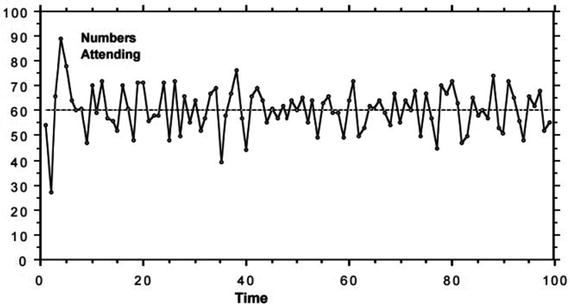
Figure 4-9. Bar attendance in the first 100 weeks in the El Farol Problem Source: ‘Inductive Reasoning and Bounded Rationality: The El Farol Problem’, Arthur, 1994

The El Farol simulation is a cornerstone in complexity circles and has been cited in a range of papers and articles over the years. In 1997, it was generalized and put into game form by two physicists, Damien Challet and Y.-C. Zhang, to create something they called, ‘The Minority Game’. The fact that the model has an economical origin and was developed by physicists, shows the interdisciplinary nature of the Minority Game.

In the original El Farol Bar problem, each individual of a population chooses whether to attend a bar on every Thursday evening. The bar has limited number of seats and can at most entertain x% of the population. If less than x% of the population go to the bar, the show in the bar is considered to be enjoyable. If not, all the people in the bar would have an unenjoyable show and staying at home is considered to be better choice than attending the bar. Arthur found the x% to be 60% and that agents used their past experience (which kept changing) to come up with a decision.

In the Minority Game, instead of using the history of past attendance, a string of binary bits which records the past few winning predictions or actions was employed as information. The predictions of the strategies were the winning choices in the next round, with no prediction about the actual size of attendance. Thus, binary information and predictions are implemented, and the winning choice is determined by the minority choice (instead of the parameter x in the Bar problem) at every round of the game. Hence the two choices are symmetric. Because of the minority rule, the population is restricted to be an odd integer in the original formulation (Yeung and Zhang, 2008).

The game goes as follows:

• A population of N agents competes in N repeated games, where N is an odd integer.

• At each round, each agent has to choose between one of the two actions, namely “0” and “1” which can also be interpreted as the ‘sell’ and ‘buy’ actions.

• The minority choices win the game at that round and all the winning agents are rewarded.

• As the game starts, every agent draws S strategies from a strategy pool which help them to make decisions throughout the game

• These strategies can be visualized in the form of tables where each strategy contains a “history column” (or “signal” column) and a “prediction column ”

  History	Prediction
  000	1
  001	0
  010	0
  011	1
  101	0
  111	1

• At every round of the game, agents make their decisions according to the strategy with the highest score at that particular moment. If there are more than one strategies with the highest score, one of these strategies is randomly employed.

The Minority Game (MG) is a simple model for the collective behaviour of agents in an idealized situation where they have to compete through adaptation for a finite resource. As the underlying strategy in this game is based on inductive reasoning and interaction between actors, there have been various updates and versions of this game. A lot of interest cumulated around the application of the game to interactions seen in financial markets as the MG refers to a simple adaptive multiagent model of financial markets.

Based on the possible interaction of investors in the financial market, some variants of the game show certain predictive abilities on real financial data. Though Minority Games are simple, they setup a framework of agent-based models from which sophisticated trading models can be built, and implementation on real trading may be possible. Although these sophisticated models are usually used for private trading and may not be open to public, Minority Games are increasingly becoming a useful tool to understand the dynamics in financial market.

Recent developments with ABCE models

The three ABCE models that have been discussed are ‘classics’ in the area of complexity economics. They are however just the tip of the iceberg. Following these seminal works, over the past few years, there has been an increasing amount of research being done in this area that is gradually attracting a more diverse set researchers from a number of fields to test, experiment and understand the economic changes that are occurring in complex financial systems. Table 4-2 offers a view of what the current areas of exploration are and the trajectories of insight that are in the process of being created. The issues being tackled are wide-ranging - from methods to identify systemic risk, to investigating the limits of fractional banking to governing policy making using ABCE insights.

Table 4-2. A short selection of ABCE papers and research projects (in no particular order)

Author(s)	Book/Research project/Articles
Gaffard & Napoletano	Agent-based models and economic policy, 2012
Kang Wei, Sun Cai-hong	Building the model of artificial stock market based on JASA, 2011
Jacky Mallett	Threadneedle: An Experimental Tool for the Simulation and Analysis of Fractional Reserve Banking Systems, 2015
Berman, Peters and Adamou	Far from Equilibrium: Wealth Reallocation in the United States
Hartmann, Guevara, Jara-Figueroa, Aristarán, Hidalgo	Linking Economic Complexity, Institutions and Income Inequality, 2015
Foxon, Köhler, Michie and Oughton	Towards a new complexity economics for sustainability, 2012
Alfarano, Fricke, Lux, Raddant	Network Approaches to Interbank Markets: Foreword, 2015
Arinaminpathy, Kapadia, May (Bank of England)	Size and complexity in model financial systems, 2012
Aymanns, Caccioli, Farmer, Tan	Taming the Basel leverage cycle, 2016
Baptista, Farmer, Hinterschweiger, Low, Tang, Uluc (Bank of England)	Macroprudential policy in an agent-based model of the UK housing market, 2016
Giovanni Dosi, Giorgio Fagiolo, Mauro Napoletano, Andrea Roventini, Tania Treibich	Fiscal and Monetary Policies in Complex Evolving Economies (2014)

The qualifications of the researchers named in the references show that a significant number of them are not economists by formal training. In fact, for most of them, their primary qualification is in the field of mathematics, physics and/or computer science. What this shows is that as complexity economics is advancing, the progress is being made a diverse set of researchers who come from a variety of scientific backgrounds. By applying the standards of scientific training to the subject of economics, these researchers are creating a new paradigm of economic thought.

This is the promise of complexity science. While economics has been in the hold with dogmatic ideologies and outdated DSGE models which have led to an inefficient understanding of economics in the past, the approaches that are being explored by complexity science offer a more inter-disciplinary approach as they base their approach from borrowing from the rich diversity of sciences. Figure 4-10 shows the contributions of various sciences and key people in their fields have allowed for this to occur.

Figure 4-10. Map of Complexity Sciences by Brian Castellani. Source: http://www.art-sciencefactory.com/complexity%20map.pdf

The previous three chapters have tried to showcase why the study of economics is in need of an upgrade. This is an essential point for as we have seen, it is based on these models and theories that policy makers make their decisions to govern our economy. This mode of thinking is what we can collectively describe as capitalism.

As we have seen, the mathematical study of economic theory was based on the models of theoretical physics. Using this point de départ, it has sought to establish itself as valid laws that can be used to explain, predict and govern economic behaviour and events. But instead of finding laws capable of being falsified through testing, economics has increasingly turned itself into an axiomatic discipline consisting of assumptions, and mathematical deductions, similar to Euclidean geometry.

But as we have seen, economics is anything but deductible and cannot be based on assumptions. As agents - be it consumers, banks, firms, or government agencies - perform different actions - be it buying, selling, trading, speculating, or investing - they are constantly innovating, forecasting and adapting to changes in the environment which is based on their interactions. This is turn creates an ever-evolving ecosystem which shows patterns that are temporary and never in a state of equilibrium. There will be a place for equilibrium in situations that are well-defined and static. But these will the exceptions to the rule of general entropy. The objective of economic theory therefore, should not be to formulate equations or to fit the agents to specific conditions. It should be to articulate insights from the changes taking place.

It is this shift in the way of looking at markets and policies that constitutes the re-definition of capitalism. A re-definition that is no longer a set of mathematical formulae but an ability to appreciate the changes occurring in an economy and to be comfortable when witnessing the creation of novel phenomenon. Economic theory in this case, would no longer be the formulation of theorems that can be applied generally, but the understanding of the forces of change that create patterns whilst acknowledging the consilience of science.

This shift is already occurring at a gradual pace and the role that complexity economics will play in this re-definition will be a central one. To highlight this point and to end this section on agent based modelling and agent based computational economics, I invite you to consider the following statements made by Jean-Claude Trichet, the president of the ECB, at an opening address at the ECB Central Banking Conference Frankfurt on 18 November 2010:

“When the crisis came, the serious limitations of existing economic and financial models immediately became apparent. Arbitrage broke down … markets froze … market participants were gripped by panic. Macro models failed to predict the crisis and … [to explain] what was happening ....”

“[In] the face of crisis, we felt abandoned by conventional tools. … The key lesson … is the danger of relying on a single tool, methodology or paradigm. The atomistic, optimising agents underlying existing models do not capture behaviour during a crisis period. Agent-based modelling … allows for more complex interactions between agents. … it dispenses with the optimisation assumption and allows for more complex interactions between agents. Such approaches are worthy of our attention we need to better integrate the crucial role played by the financial system into our macroscopic models.”

"I would very much welcome inspiration from other disciplines: physics, engineering, psychology, biology. Bringing experts from these fields together with economists and central bankers is potentially very … valuable."

"A large number of aspects of the observed behaviour of financial markets is hard to reconcile with the efficient market hypothesis… But a determinedly empirical approach - which places a premium on inductive reasoning based on the data, rather than deductive reasoning grounded in abstract premises or assumptions - lies at the heart of these methods … simulations will play a helpful role."

Putting it all together

"Economic theorists, like French chefs in regard to food, have developed stylized models whose ingredients are limited by some unwritten rules. Just as traditional French cooking does not use seaweed or raw fish, so neoclassical models do not make assumptions derived from psychology, anthropology, or sociology. I disagree with any rules that limit the nature of the ingredients in economic models", George Akerlof, An Economic Theorist’s Book of Tales (1984)

It would seem that we have drifted from the topic of the Blockchain whilst endeavouring to grasp the basics of complexity economics. But actually, we were just setting the stage to the final point to be made in this book. The Blockchain is not a panacea. It is a tool and like any good tool, it is versatile and works better when it is part of a tool kit. Complexity economics is another tool that will need to be used to re- define capitalism, and to the precocious reader, the connection between the Blockchain and Complexity Economics must be evident already.

The Blockchain is many things - it is a shared ledger, a medium to issue money, a means of exchanging value in a decentralized way and a consensus mechanism that offers the possibility of achieving global financial inclusion. But what it is more than anything else is the digital embodiment of trust. A Blockchain is in essence, a codified truth-verification machine that has the ability to commoditize trust through a protocol on a decentralized network. The key word in that phrase is decentralized because markets are decentralized. An organization may be centralized with various hierarchies. But markets are decentralized and as we have seen in chapter 2 (refer the part on FinTech), and are getting increasingly so.

In decentralized markets with multiple agents, trust becomes a key factor as it has a cost associated to it. Owing to uncertainty, opportunism and limited information (bounded rationality), the lack of trust between agents limits the number of interactions and bonds that are formed in a network. This hesitation to form links based on lack of trust has been extensively studied in the field of transaction cost theory (also called new institutional economics) which was developed by Ronal Coase in 1937.

Transactional cost theory (TCT) is the branch of economics that deals with the costs of transactions and the institutions that are developed to govern them. It studies the cost of economic links and the ways in which agents organize themselves to deal with economic interactions. Coase realized that economic transactions are costly. In his seminal paper, ‘The Nature of the Firm’, Coase noted that while economies involve plenty of planning, a large part of this planning is not coordinated by the price system and takes place within the boundaries of the firm (Hidalgo, 2015). As firms have hierarchies, most interactions within a firm are political. This creates boundaries of power that influence transactions and interactions causing them to deviate from the clear-cut dynamics of market price mechanisms. This is seen in the form of contracts, inspections, disputes, negotiations, etc. These boundaries in turn rack up costs and the greater the cost associated with a transaction, the more friction associated with making the transaction.

But trust is an essential element in any network as it allows for the transfer of information, knowledge and knowhow. If there is a greater amount of trust in the network, links are formed more easily and transactions occur with a greater amount of fluidity thus increasing the network size. By reducing the cost of links and by providing porous boundaries that allow for greater exchanges of knowledge and knowhow high trust networks are able to adapt faster to changes in markets and technologies. This phenomenon has been discussed in great detail in the book ‘Why Information Grows’ (2015), by César Hidalgo.

Using complexity models, Hidalgo develops TCT to show that in economic networks, the cheaper the link, the larger the network. Using Coase’s work, he shows that trust is an essential element of social capital as it is the glue that is needed to maintain and form large networks which allows for the spread of knowledge and knowhow that are accumulated in these networks. Trust contributes to network size by reducing the cost of links.The links are therefore created more easily as the creation of new is not considered risky. Low trust networks on the other hand produce networks with less porous boundaries that limit their long-term adaptability. He concludes his book by stating that the growth of economies is based on the growth of information and those countries are that are better at making information grow are more prosperous. In sum, the greater the level of trust and the more complex the economy, the more prosperous it is.

As Blockchains are a mechanism that allow for the crypto-enforced execution of the agreed contracts through consensus and transparency, they offer a control mechanism that reduces the need of trust to a large degree (Davidson et al., 2016). As the adoption of the Blockchain continues to rise, the potential that it offers to governments is not just in terms of increased transparency, but also as a way of increasing the trust in the economy. In a world beset by technological unemployment and inequality, the Blockchain offers governments a number of ways to rethink their functions and the institutions that make up their economy.

Moreover, they do not have to be passive witnesses to the transactional data that is flowing on these decentralized networks. By using the techniques of complexity economics, they can use this data to see how the significant elements of an economy are transacting within an economy and how their interactions are changing the ecosystem. Using this information, they can create simulations to see what reactions monetary and fiscal policies (i.e.: changes in the environment) will create and how the ripples of these environmental changes will affect smaller agents in the economy. Monetary and Fiscal policy will no longer have to be reactive in nature, but could be made perspective instead.

Of course, moving to such kind of a framework will not be an overnight process as it forces us to rethink market fundamentals and economic policy making from the ground up. But as we have seen in this chapter, this has already begun and there is a whole new field of scientific enquiry that is reformulating the way we think of the fundamentals of economic theory. The way this process can be enacted and the challenges it will create at the micro, meso and macro levels is a subject that will need to be addressed in detail in the years to come. It is beyond the scope of this book to provide such an encyclopaedic overview of all the issues that are related to this endeavour. As mentioned from the very beginning, the objective of this book has been to change the direction of the conversation that we have today with regards to capitalism. As we have seen in these four chapters, this conversation has already begun in some academic and policy circles. My objective has been to give these conversations a collective voice.

Conclusion

‘I think the next century will be the century of complexity’, Stephen Hawking, January 2000

Economics and Ecology share a common etymological origin. They both derive themselves from the Greek word for household - ‘Oikos’. ‘Logy’, derives itself from another Greek word, ‘Logos’ (from legein), which means to gather, count, or account. ‘Nomos’, on the other hand, derives itself from the Greek ‘Nemein’, which means to distribute or to manage. Thus, ecology at the root means the logic of the dwelling place, or the story of where we live. Economy is eco plus nomos, which means household management (oikonomia Greek).

It is surprising to realise that although these two words share the same origin, they have become completely separated over the course of time. This is not just from the perspective of how they are studied, but also in the way the they have been pitted against each other. As increased financialization, excessive consumerism and growing debt and inequality continue their upward curve, the problems of the climate change and the detriment of the ecology continue to rise as well. I have often pondered if our ecology would be in its present state had we begun the study of economics using the perspectives of the ecologist rather than the tools of the physicist (Walrasian approach).

The atavistic disciplinary chauvinism of economics also seems to ignore its Greek cousin, Democracy. Capitalism and Democracy are often seen to go hand in hand and that they are natural allies. Most capitalistic states are democracies are to a large extent capitalism and democracy are accepted in spite of all their shortcomings as there is no sound ideological alternative to replace them. But as the world gets increasingly complex with advances in technologies, such as the Blockchain, we need to take heed as to what the implications of these technologies are and how do we study the implications of these changes.

This feat cannot be achieved by solely focusing on the applications of technology. It requires that we also have a healthy understanding of economic history. As we have seen in this book, solution proposals to problems that face us today were made decades ago by economists who had a heathy appreciation of the limitations of economic theory and the definition of capitalism in the context of a liberal democracy. Adam Smith, David Ricardo, Karl Marx and all the way to Schumpeter tried to stay faithful to this approach. Yanis Varoufakis best summed up this dilemma at a speech he made at the New School in April 2016,

"Capitalism without the state is like Christianity without hell. It does not work … The phenomenon of considering capitalism and democracy as natural bedfellows is a very recent phenomenon …[But] unless we approach it [the study of capitalism] via …a simultaneous study of economic history … or the history of capitalism, the evolution of the conflict between social relations of production and technologies on one hand and the evolution of our ideas about the world that is being shaped by this historical evolutionary process [on the other hand]…unless we study the past, the present and the potentialities for the future through this prism, we have no chance of using a mathematized approach in order to secure any handle on the reality in which we find ourselves.’’

Where capitalism is headed today is a step before it became communism - a bourgeois liberal democracy. It is our collective responsibility and vicarious liability to use technologies that are changing the definition of capitalism to create a more sensible, just and scientifically accurate version of it.

In a world of information where the answer to any question can be found, real value is derived from asking the right question. The Blockchain is a tool for transferring value and recording this information. Its time we started asking the right questions of what can we do with this tool.

Some Final Notes

The remaining sections provide further perspective to topics covered earlier in the chapter:

• Section “Technology and Invention: A Combinatorial Process”

• Sidebar 4-1 : “A rationale for rational expectations”

• Section “The Mathematical Wizardry of Equilibrium Economic Models”

A brief history of computing

Sources: The Computing Universe: A Journey through a Revolution, Tony Hey and Gyuri Pápay, (2014); A History of Modern Computing (2nd Edition), Paul E. Ceruzzi, (1998).

The story of computing and computers goes back to the early 19^th century when Charles Babbage, a mathematician who was trained at Cambridge, first had the idea to create a machine to calculate logarithmic tables. In 1819, shortly after leaving Cambridge, Babbage was working with the astronomer John Herschel and carrying out arithmetical calculations by hand. As the process was tedious and fraught with errors, Babbage hit upon the idea of making a machine that could perform routine calculations by following precise arithmetical procedures. This led Babbage to begin working on something later he called the Difference Engine - a machine that would calculate astronomical and navigational tables and record the results on metal plates (so that they could be used directly for printing). The project was later funded by the U.K. government and was developed by Babbage and Joseph Clement for well over a decade. It was cancelled in 1842, owing to differences between Babbage and Clement, and had cost the government over £ 17,000 - a princely sum in those days.

Babbage’s Difference Engine was the first special-purpose calculator and the basis for his next idea, the Analytical Engine. Although he never secured the funds to develop the second project, the ideas in its design (documented in over 6000 pages of notes, hundreds of engineering drawings and operational charts) are the basis for today modern computers. These included a separated section for calculation (what we today refer to as a Central Processing Unit (CPU)), another section for storing data (or a memory) and a method of providing instructions to the machine (a programming language). Ada Lovelace, who corresponded with Babbage, also played an influential role in developing programming languages by emphasising that the Analytical Machine could manipulate symbols as well as numerical calculations. However, the real advances in programming languages came from George Boole who devised a language for describing and manipulating complex logical statements for determining the statements were true or false. Although Boole, who created Boolean Algebra, did not himself work in computing, his ideas of logical operations (AND, OR and NOT) were later used to improve the performance of later computers and in the creation of logic gates.

In the mid-1930s, Vannevar Bush an American engineer, inventor and head of the U.S. Office of Scientific Research and Development (OSRD) during the Second World War, had created an analog computer known as the Differential Analyser. This computer was used to solve ordinary differential equations which would help calculate the trajectories of shells. It consisted of multiple rotating disks and cylinders driven by electric motors linked together with metal rods that were manually set up (sometime taking up to two days) to solve any differential equation problem. Vannevar had recruited Claude Shannon (known today as the father of information theory), a young graduate who specialised symbolic logic.

Although the Differential Analyzer was a mechanical machine with moving parts, Shannon identified it as a complicated control circuit with relays. Shannon thus began creating the first generation of circuit designs and in the process, was able to transform information into a quantity that could be subjected to manipulation by a machine. Using Boolean algebra, logic gates and binary arithmetic (bits and bytes), Shannon was able to represent all types of information by numbers and in the process created the foundations for today’s modern information theory. It is for this reason that he is referred to as the father of information technology.

As World War Two began in 1939, these advances in information technology had been adopted by various militaries to communicate sensitive information. Cryptography became a suitable way of camouflaging information and led to the creation of the Enigma machine. Luckily for the Allies, hope lay in the form of some work that had been done a few years earlier by another Cambridge mathematician, Alan Turing. Along with his mentor, Max Newman, Turing set about designing and building automated machines (Turing Machines) that could decrypt secret German military communications (as documented in the popular movie, ‘The Imitation Game’). However, owing to an obsession for secrecy during the war years and for several years after that, the achievements made by Turing and the team at Bletchley Park in computer development was kept hidden from view.

Instead of Turing Machines, over the same time period, a machine called the ENIAC (Electronic Numerical Integrator And Computer) was being developed by John Mauchly and Presper Eckert across the Atlantic. Mauchly, a physicist, who was interested in meteorology tried to develop a weather prediction model. But he soon realized that this would not be possible without some kind of automatic calculating machine. As a result, he developed the concept of an electronic computer using vacuum tubes. It was during the time of developing ENIAC that he met the renowned polymath, John von Neumann, and with his help went on to design a stored-program computer, the EDVAC (Electronic Discrete Variable Automatic Computer), the first binary computer (ENIAC was decimal). See Figure 4-11.

Figure 4-11. General design of the Electronic Discrete Variable Automatic Computer. Reference Source: ‘The von Neumann Architecture’, The Computing Universe, 2014

From an abstract architecture perspective, von Neumann’s design is logically equivalent to Turing’s Universal Turing Machine. In fact, von Neumann had read Turing’s theoretical papers prior to designing his machine. Ultimately it was this simple design that was built upon by successive generations of computer scientists and led to the design of computers with multiple processors and the creation of parallel computing.

The period following the war saw great strides being made in the hardware of computers. From the early days of vacuum tubes and mercury delay-lines (a thin mercury filled tube that stored electronic pulses that represented binary data points - a pulse represented 1; no pulse represented 0), computing hardware saw the inculcation of the Magnetic Core Memory and the creation of the Hard Disk. But an equal if not more diverse progress was also made in the space of software development. From punch cards and simple logic gates, software’s ability to access, compute and handle data underwent leaps and bounds of progress. Languages such as COBOL and FORTRAN (FORmula TRANslation), helped in the creation of early operating systems and over the years we have seen the rise software design and programming languages and such as BASIC, LISP, SIMULA, C, C++, UML, Unix, Linux, etc… Ultimately it was these advents that led to the construction of distributed communication networks, the internet and the worldwide web.

The history of computing cannot be summarised in a short blurb and readers are encouraged to have a look at the excellent books cited in the references cited at the beginning of this note for a more detailed understanding. The point of providing this short note is to highlight how technology grows. With every advance in different sectors of the natural sciences, technology borrows from its ancestors and novelty comes from combining cumulative small changes in different technological families. Computers may have started from mathematics, but it is only the evolution in physics, chemistry and, more recently, biology that have allowed us to develop today’s technologies. Without this method of scientific enquiry and consilience of science, we would not have today’s technologies and definitely would not be talking about the Blockchain. As affective computing gains strides, the role that human emotions will play in the evolution of technology will gain an increasingly important role.

Types of Macroeconomic Models

Source: ‘The Role of Expectations in the FRB/US Macroeconomic Model’, Flint Brayton, Eileen Mauskopf, David Reifschneider, Peter Tinsley, and John Williams (1997).

FRB/US is one of many macroeconomic models that have been developed over the past 30 years. Macroeconomic models are systems of equations that summarize the interactions among such economic variables as gross domestic product (GDP), inflation, and interest rates. These models can be grouped into several types:

Traditional structural modelstypically follow the Keynesian paradigm featuring sluggish adjustment of prices. These models usually assume that expectations are adaptive but subsume them in the general dynamic structure of specific equations in such a way that the contribution of expectations alone is not identified. The MPS and Multi-Country (MCM) models formerly used at the Federal Reserve Board are examples.

Rational expectations structural modelsexplicitly incorporate expectations that are consistent with the model’s structure. Examples include variants of the FRB/US and FRB/MCM models currently used at the Federal Reserve Board, Taylor’s multi-country model, and the IMF’s Multimod.

Equilibrium business-cycle modelsassume that labor and goods markets are always in equilibrium and that expectations are rational. All equations are closely based on assumptions that households maximize their own welfare and firms maximize profits. Examples are models developed by Kydland and Prescott and by Christiano and Eichenbaum.

Vector autoregression (VAR) modelsemploy a small number of estimated equations to summarize the dynamic behaviour of the entire macroeconomy, with few restrictions from economic theory beyond the choice of variables to include in the model. Sims is the original proponent of this type of model.

Cellular automata (CA): “Automaton” (plural: “automata") is a technical term used in computer science and mathematics for a hypothetical machine that changes its internal state based on inputs and its previous state. (Sayama, 2015). A cellular automaton consists of a regular grid of cells, each in one of a finite number of states, such as on and off. Each cell is surrounded by a set of cells called it neighbourhood. At a particular time (t), the cell and its neighbourhood cells are in a specific state according to some fixed mathematical rules. These rules also determine how the cells will update over time and how they interact with their neighbourhood. As time progresses from (t) to (t + t), a new generation of cells is created by interacting with each other and updating simultaneous.

The original idea of CA was invented by John von Neumann and Stanisław Ulam. They invented this modelling framework, which was the very first to model complex systems, in order to describe self-reproductive and evolvable behaviour of living systems. CA is used in computability theory, mathematics, physics, complexity science, theoretical biology and microstructure modelling.

Neural networks: More specifically Artificial Neural Networks (ANN) , are processing devices (they can be algorithms or actual hardware) that are loosely modelled after the neuronal structure of the brains’ cerebral cortex but on smaller scales (Figure 4-12).

Figure 4-12. Sketch of a biological neural network Source: Boundless Psychology, 2013

The origin of modern ANNs is based on a mathematical model of the neuron called the perceptron introduced by Frank Rosenblatt in 1957 (Papay and Hey, 2015). As it can be seen in Figure 4-13, the model closely resembles the structure of the neuron with inputs resembling dendrites.

Figure 4-13. Representation of an artificial neuron with inputs, connection weights, and the output subject to a threshold function Source: ‘The computing universe’, Gyuri Papay and Tony Hey, 2015

In the original model made by Warren McCulloch and Walter Pitts, the inputs were either 0 or 1. Each dendrite/input also had a weight of +1 and - 1. The input was thus multiplied by its weight and the sum of the inputs was then fed to a model. The perceptron thus takes several binary inputs, I₁, I₂, …I_N, and produces a single binary output. If the output is greater than a set threshold level, then the model delivers a certain output. This can be mathematically interpreted as:

Based on this initial schema, the perceptron model developed to allow both the inputs to the neurons and the weights to take on any value. ANN is nothing more than interconnected layers of perceptron’s as seen in Figure 4-14.

Figure 4-14. Perceptron’s interconnected layers Image source: The computing universe, Gyuri Papay and Tony Hey, 2015

By varying the weights and the threshold, we can get different models of decision-making. The outputs from a hidden layer can also be fed into another hidden layer of perceptron’s. The first layer of column of perceptron’s makes very simple decisions, by weighing the input evidence. These outputs are then fed to a second layer of perceptron’s which make a decision by weighing up the results from the first layer of decision-making. By following this method, a perceptron in the second layer can make a decision at a more complex and more abstract level than perceptron’s in the first layer. If a third layer is involved, then the decisions can be made by those perceptron’s will be even more complex. In this way, a many- layer network of perceptron’s can engage in sophisticated decision making. The greater the number of layers of perceptron’s, the higher the decision-making ability (Figure 4-14).

Figure 4-15. Milti-layer network of perceptrons Source: http://neuralnetworksanddeeplearning.com/

Genetic algorithms: A Genetic algorithm (GA) is a heuristic search method used in artificial intelligence and computing inspired by Darwin’s theory about evolution. It is used for finding optimized solutions to search problems based on the theories of natural selection and evolutionary biology, i.e.: selection, mutation, inheritance and recombination.

GAs are based on the classic view of a chromosome as a string of genes. R.A. Fisher used this view to found mathematical genetics, providing mathematical formula specifying the rate at which particular genes would spread through a population (Fisher, 1958). They key elements of Fisher’s formulation are (Holland, 2012):

1. A specified set of alternatives for each gene, thereby specifying the permissible strings of genes that can evolve.

2. A generation-by-generation view of evolution where, at each stage, a population of individuals produces a set of offspring that constitutes the next generation.

3. A fitness function that assigns to each string of alternatives, the number of offspring the individual carrying that chromosome will contribute to the next generation.

4. A set of genetic operators, particularly mutation in Fisher’s formulation, that modify the offspring of an individual so that the next generation differs from the current generation.

When solving constrained and unconstrained optimization problems, a classical algorithm generates a single data point at each iteration. The sequence of data points then approaches an optimal solution. A GA on the other hand uses a process similar to natural selection - it repeatedly modifies a population of individual solutions and at each step, randomly selects data points from the current population of points and uses them as ‘parents’ to produce the children for the next generation. Over successive generations, the population ‘evolves’ toward an optimal solution (Holland, 2012).

Although randomised, GAs are by no means random, instead they exploit historical information to direct the search into the region of better performance within the search space. GAs simulate the survival of the fittest among individuals over consecutive generations for solving a problem. Each generation consists of a population of character strings that are analogous to the chromosome that we see in our DNA. Each individual represents a point in a search space and a possible solution. The individuals in the population are then made to go through a process of evolution.

GAs are used for searching through large and complex data sets as they are capable of finding reasonable solutions to complex issues by solving unconstrained and constrained optimization issues. They are used to solve problems that are not well suited for standard optimization algorithms, including problems in which the objective function is discontinuous, nondifferentiable, stochastic, or highly nonlinear. GAs also work particularly well on mixed (continuous and discrete) combinatorial problems, as they are less susceptible to getting ‘stuck’ at local optima than classical gradient search methods. However, they tend to be computationally expensive.