
Machine learning is a subfield of computer science that evolved from the study of pattern recognition and computational learning theory in Artificial Intelligence (AI).
Let’s look at a few other versions of definitions that exist for machine learning:
In 1959, Arthur Samuel, an American pioneer in the field of computer gaming, machine learning, and artificial intelligence has defined machine learning as a “Field of study that gives computers the ability to learn without being explicitly programmed.”
Machine learning is a field of computer science that involves using statistical methods to create programs that either improve performance over time, or detect patterns in massive amounts of data that humans would be unlikely to find.
Machine Learning explores the study and construction of algorithms that can learn from and make predictions on data. Such algorithms operate by building a model from example inputs in order to make data driven predictions or decisions, rather than following strictly static program instructions.
All the above definitions are correct; in short, “Machine Learning is a collection of algorithms and techniques used to create computational systems that learn from data in order to make predictions and inferences.”
Machine learning application area is abounding. Let’s look at some of the most common day-to-day applications of Machine Learning that happens around us.
Recommendation System: YouTube brings videos for each of its users based on a recommendation system that believes that the individual user will be interested in. Similarly Amazon and other such e-retailers suggest products that the customer will be interested in and likely to purchase by looking at the purchase history for a customer and a large inventory of products.
Spam detection: Email service providers use a machine learning model that can automatically detect and move the unsolicited messages to the spam folder.
Prospect customer identification: Banks, insurance companies, and financial organizations have machine learning models that trigger alerts so that organizations intervene at the right time to start engaging with the right offers for the customer and persuade them to convert early. These models observe the pattern of behavior by a user during the initial period and map it to the past behaviors of all users to identify those that will buy the product and those that will not.
History and Evolution
Machine learning is a subset of Artificial Intelligence (AI), so let’s first understand what AI is and where machine learning fits within its wider umbrella. AI is a broad term that aims at using data to offer solutions to existing problems. It is the science and engineering of replicating, even surpassing human level intelligence in machines. That means observe or read, learn, sense, and experience.
The AI process loop is as follows in Figure 2-1:
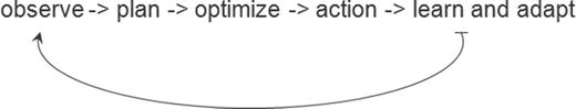
Figure 2-1. AI process loop
Observe – identify patterns using the data
Plan – find all possible solutions
Optimize – find optimal solution from the list of possible solutions
Action – execute the optimal solution
Learn and Adapt – is the result giving expected result, if no adapt
The AI process loop discussed above can be achieved using intelligent agents. A robotic intelligent agent can be defined as a component that can perceive its environment through different kinds of sensors (camera, infrared, etc.), and will take actions within the environment through efforts. Here robotic agents are designed to reflect humans. We have different sensory organs such as eyes, ears, noses, tongues, and skin to perceive our environment and organs such as hands, legs, and mouths are the effectors that enable us to take action within our environment based on the perception.
A detailed discussion on designing the agent has been discussed in the book Artificial Intelligence, A Modern Approach by Stuart J. Russell and Peter Norvig in 1995. Figure 2-2 shows a sample pictorial representation.
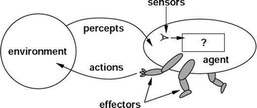
Figure 2-2. Depict of robotic intelligent agent concept that interacts with its environment through sensors and effectors
To get a better understanding of the concept, let’s look at an intelligent agent designed for a particular environment or use case. Consider designing an automated taxi driver. See Table 2-1.
Table 2-1. Example intelligent agent components
Intelligent Agent’s Component Name | Description |
|---|---|
Agent Type | Taxi driver |
Goals | Safe trip, legal, comfortable trip, maximize profits, convenient, fast |
Environment | Roads, traffic, signals, signage, pedestrians, customers |
Percepts | Speedometer, microphone, GPS, cameras, sonar, sensors |
Actions | Steer, accelerate, break, talk to passenger |
The taxi driver robotic intelligent agent will need to know its location, the direction in which its traveling, the speed at which its traveling, what else is on the road! This information can be obtained from the percepts such as controllable cameras in appropriate places, the speedometer, odometer, and accelerometer. For understanding the mechanical state of the vehicle and engine, it needs electrical system sensors. In addition a satellite global positioning system (GPS) can help to provide its accurate position information with respect to an electronic map and infrared/sonar sensors to detect distances to other cars or obstacles around it. The actions available to the intelligent taxi driver agent are the control over the engine through the pedals for accelerating, braking, and steering for controlling the direction. There should also be a way to interact with or talk to the passengers to understand the destination or goal.
In 1950, Alan Turing a well-known computer scientist proposed a test known as Turing test in his famous paper “Computing Machinery and Intelligence.” The test was designed to provide a satisfactory operational definition of intelligence, which required that a human being should not be able to distinguish the machine from another human being by using the replies to questions put to both.
To be able to pass the Turing test , the computer should possess the following capabilities:
Natural language processing, to be able to communicate successfully in a chosen language
Knowledge representation, to store information provided before or during the interrogation that can help in finding information, making decisions, and planning. This is also known as ‘Expert System’
Automated reasoning (speech), to use the stored knowledge map information to answer questions and to draw new conclusions where required
Machine learning, to analyzing data to detect and extrapolate patters that will help adapt to new circumstances
Computer vision to perceive objects or the analyzing of images to find features of the images
Robotics devices that can manipulate and interact with its environment. That means to move the objects around based on the circumstance
Planning, scheduling, and optimization, which means figuring ways to make decision plans or achieve specified goals, as well as analyzing the performance of the plans and designs
The above-mentioned seven capability areas of AI have seen a great deal of research and growth over the years. Although many of the terms in these areas are used interchangeably, we can see from the description that their objectives are different. Particularly machine learning has seen a scope to cut across all the seven areas of AI. See Figure 2-3.
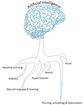
Figure 2-3. Artificial Intelligence Areas
Artificial Intelligence Evolution
Let’s understand briefly the artificial intelligence past, present, and future.
 | Artificial Narrow Intelligence ( ANI ) : Machine intelligence that equals or exceeds human intelligence or efficiency at a specific task. An example is IBM’s Watson, which requires close participation of subject matter or domain experts to supply data/information and evaluate its performance. |
 | Artificial General Intelligence ( AGI ) : A machine with the ability to apply intelligence to any problem for an area, rather than just one specific problem. Self-driving cars are a good example of this. |
 | Artificial Super Intelligence ( ASI ) : An intellect that is much smarter than the best human brains in practically every field, general wisdom, social skills, and including scientific creativity. The key theme over here is “don’t model the world, model the mind”. |
Different Forms
Is Machine Learning the only subject in which we use data to learn and use for prediction/inference?
To answer the above questions, let’s have a look at the definition (Wikipedia) of the few other key terms (not an exhaustive list) that are often heard relatively:
Statistics: It is the study of the collection, analysis, interpretation, presentation, and organization of data.
Data Mining: It is an interdisciplinary subfield of computer science. It is the computational process of discovering patterns in large data sets (from data warehouse) involving methods at the intersection of artificial intelligence, machine learning, statistics, and database systems.
Data Analytics: It is a process of inspecting, cleaning, transforming, and modeling data with the goal of discovering useful information, suggesting conclusions, and supporting decision making. This is also known as Business Analytics and is widely used in many industries to allow companies/organization to use the science of examining raw data with the purpose of drawing conclusions about that information and make better business decisions.
Data Science: Data science is an interdisciplinary field about processes and systems to extract knowledge or insights from data in various forms, either structured or unstructured, which is a continuation of some of the data analysis fields such as statistics, machine learning, data mining, and predictive analytics, similar to Knowledge Discovery in Databases (KDD).
Yes, from the above definitions it is clear and surprising to find out that Machine Learning isn’t the only subject in which we use data to learn from it and use further for prediction/inference. Almost identical themes, tools, and techniques are being talked about in each of these areas. This raises a genuine question about why there are so many different names with lots of overlap around learning from data? What is the difference between these?
The short answer is that all of these are practically the same. However, there exists a subtle difference or shade of meaning, expression, or sound between each of these. To get a better understanding we’ll have to go back to the history of each of these areas and closely examine the origin, core area of application, and evolution of these terms.
Statistics
German scholar Gottfried Achenwall introduced the word “Statistics” in the middle of the 18th century (1749). Usage of this word during this period meant that it was related to the administrative functioning of a state, supplying the numbers that reflect the periodic actuality regarding its various area of administration. The origin of the word statistics may be traced to the Latin word “Status” (“council of state”) or the Italian word “Statista” (“statesman” or “politician”); that is, the meaning of these words is “Political State” or a Government. Shakespeare used a word Statist in his drama Hamlet (1602). In the past, the statistics were used by rulers that designated the analysis of data about the state, signifying the “science of state.”
In the beginning of the 19th century, statistics attained the meaning of the collection and classification of data. The Scottish politician, Sir John Sinclair, introduced it to the English in 1791 in his book Statistical Account of Scotland. Therefore, the fundamental purpose of the birth of statistics was around data to be used by government and centralized administrative organizations to collect census data about the population for states and localities.
Frequentist
John Graunt was one of the first demographers and is our first vital statistician. He published his observation on the Bills of Mortality (in 1662), and this work is often quoted as the first instance of descriptive statistics. He presented vast amounts of data in a few tables that can be easily comprehended, and this technique is now widely known as descriptive statistics. In it we note that weekly mortality statistics first appeared in England in 1603 at the Parish-Clerks Hall. We can learn from it that in 1623, of some 50,000 burials in London, only 28 died of the plague. By 1632, this disease had practically disappeared for the time being, to reappear in 1636 and again in the terrible epidemic of 1665. This exemplifies that the fundamental nature of descriptive statistics is counting. From all the Parish registers, he counted the number of persons who died, and who died of the plague. The counted numbers every so often were relatively too large to follow, so he also simplified them by using proportion rather than the actual number. For example, the year 1625 had 51,758 deaths and of which 35,417 were of the plague. To simplify this he wrote, “We find the plague to bear unto the whole in proportion as 35 to 51. Or 7 to 10.” With these he is introducing the concept that the relative proportions are often of more interest than the raw numbers. We would generally express the above proportion as 70%. This type of conjecture that is based on a sample data’s proportion spread or frequency is known as “frequentist statistics.” . Statistical hypothesis testing is based on inference framework, where you assume that observed phenomena are caused by unknown but fixed processes.
Bayesian
In contract Bayesian statistics (named after Thomas Bayes), it describes that the probability of an event, based on conditions that might be related to the event. At the core of Bayesian statistics is Bayes’s theorem, which describes the outcome probabilities of related (dependent) events using the concept of conditional probability. For example, if a particular illness is related to age and life style, then applying a Bay’s theorem by considering a person’s age and life style more accurately increases the probability of that individual having the illness can be assessed.
Bayes theorem is stated mathematically as the following equation:
Where A and B are events and P (B) ≠ 0
P (A) and P (B) are the probabilities of observing A and B without regard to each other.
P (A | B), a conditional probability, is the probability of observing event A given that B is true.
P (B | A) is the probability of observing event B given that A is true.
For example, a doctor knows that lack of sleep causes migraine 50% of the time. Prior probability of any patient having lack of sleep is 10000/50000 and prior probability of any patient having migraine is 300/1000. If a patient has a sleep disorder, let’s apply Bayes’s theorem to calculate the probability he/she is having a migraine.
P (Sleep disorder | Migraine) = P(Migraine | Sleep disorder) * P(Migraine) / P(Sleep disorder)
P (Sleep disorder | Migraine) = .5 * 10000/50000 / (300/1000) = 33%
In the above scenario, there is a 33% chance that a patient with a sleep disorder will also have a migraine problem.
Regression
Another major milestone for statisticians was the regression, which was published by Legendre in 1805 and by Guass in 1809. Legendre and Gauss both applied the method to the problem of determining, from astronomical observations, the orbits of bodies about the Sun, mostly comets, but also later the then newly discovered minor planets. Gauss published a further development of the theory of least squares in 1821. Regression analysis is an essential statistical process for estimating the relationships between factors. It includes many techniques for analyzing and modeling various factors, and the main focus here is about the relationship between a dependent factor and one or many independent factors also called predictors or variables or features. We’ll learn about this more in the fundamentals of machine learning with scikit-learn.
Over time the idea behind the word statistics has undergone an extraordinary transformation. The character of data or information provided has been extended to all spheres of human activity. Let’s understand the difference between two terms quite often used along with statistics, that is, 1) data and 2) method. Statistical data is the numerical statement of facts, whereas statistical methods deal with information of the principles and techniques used in collecting and analyzing such data. Today, statistics as a separate discipline from mathematics is closely associated with almost all branches of education and human endeavor that are mostly numerically representable. In modem times, it has innumerable and varied applications both qualitatively and quantitatively. Individuals and organizations use statistics to understand data and make informed decisions throughout the natural and social sciences, medicine, business, and other areas. Statistics has served as the backbone and given rise to many other disciplines, which you’ll understand as you read further.
Data Mining
The term “Knowledge Discovery in Databases” (KDD) is coined by Gregory Piatetsky-Shapiro in 1989 and also at the same time he cofounded the first workshop named KDD. The term “Data mining” was introduced in the 1990s in the database community, but data mining is the evolution of a field with a slightly long history.
Data mining techniques are the result of research on the business process and product development. This evolution began when business data was first stored on computers in the relational databases and continued with improvements in data access, and further produced new technologies that allow users to navigate through their data in real time. In the business community, data mining focuses on providing “Right Data” at the “Right Time” for the “Right Decisions.” This is achieved by enabling a tremendous amount of data collection and applying algorithms to them with the help of distributed multiprocessor computers to provide real-time insights from data.
We’ll learn more about the five stages proposed by KDD for data mining in the section on the framework for building machine learning systems.
Data Analytics
Analytics have been known to be used in business, since the time of management movements toward industrial efficiency that were initiated in late 19th century by Frederick Winslow Taylor, an American mechanical engineer. The manufacturing industry adopted measuring the pacing of the manufacturing and assembly line, as a result revolutionizing industrial efficiency. But analytics began to command more awareness in the late 1960s when computers had started playing a dominating role as organizations’ decision support systems. Traditionally business managers were making decisions based on past experiences or rules of thumb, or there were other qualitative aspects to decision making; however, this changed with development of data warehouses and enterprise resource planning (ERP) systems . The business managers and leaders considered data and relied on ad hoc analysis to affirm their experience/knowledge-based assumptions for daily and critical business decisions. This evolved as data-driven business intelligence or business analytics for the decision-making process was fast adopted by organizations and companies across the globe. Today, businesses of all sizes use analytics. Often the word “Business Analytics” is used interchangeably for “Data Analytics” in the corporate world.
In order for businesses to have a holistic view of the market and how a company competes efficiently within that market to increase the RoI (Return on Investment), requires a robust analytic environment around the kind of analytics that is possible. This can be broadly categorized into four types. See Figure 2-4.
Descriptive Analytics
Diagnostic Analytics
Predictive Analytics
Prescriptive Analytics
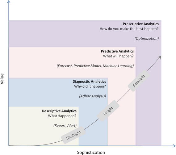
Figure 2-4. Data Analytics Types
Descriptive Analytics
They are the analytics that describe the past to tell us “What has happened?” To elaborate, as the name suggests, any activity or method that helps us to describe or summarize raw data into something interpretable by humans can be termed ‘Descriptive Analytics’. These are useful because they allow us to learn from past behaviors, and understand how they might influence future outcomes.
The statistics such as arithmetic operation of count, min, max, sum, average, percentage, and percent change, etc., fall into this category. Common examples of descriptive analytics are a company’s business intelligence reports that cover different aspects of the organization to provide historical hindsights regarding the company’s production, operations, sales, revenue, financials, inventory, customers, and market share.
Diagnostic Analytics
It is the next step to the descriptive analytics that examines data or information to answer the question, “Why did it happen?,” and it is characterized by techniques such as drill-down, data discovery, data mining, correlations, and causation. It basically provides a very good understanding of a limited piece of the problem you want to solve. However, it is very laborious work as significant human intervention is required to perform the drill-down or data mining to go deeper into the data to understand why something happened or its root cause. It focuses on determining the factors and events that contributed to the outcome.
For example, assume a retail company’s hardlines (it’s a category usually encompassing furniture, appliance, tools, electronics, etc.) sales performance is not up to the mark in certain stores and the product line manager would like to understand the root cause. In this case the product manager may want to look backward to review past trends and patterns for the product line sales across different stores based on its placement (which floor, corner, aisle) within the store. It’s also to understand if there is any causal relationship with other products that are closely kept with it. Look at different external factors such as demographic, season, macroeconomic factors separately as well as in unison to define relative ranking of related variables based on concluded explanations. To accomplish this there is not a clearly defined set of ordered steps defined, and it depends on the experience level and thinking style of the person carrying out the analysis.
There is a significant involvement of the subject matter expert and the data/information may need to be presented visually for better understanding. There is a plethora of tools: for example, Excel, Tableau, Qlikview, Spotfire, and D3, etc., are available build tools that enable diagnostic analytics.
Predictive Analytics
It is the ability to make predictions or estimations of likelihoods about unknown future events based on the past or historic patterns. Predictive analytics will give us insight into “What might happen?”; it uses many techniques from data mining, statistics, modeling, machine learning, and artificial intelligence to analyze current data to make predictions about the future.
It is important to remember that the foundation of predictive analytics is based on probabilities, and the quality of prediction by statistical algorithms depends a lot on the quality of input data. Hence these algorithms cannot predict the future with 100% certainty. However, companies can use these statistics to forecast the probability of what might happen in the future and considering these results alongside business knowledge would result in profitable decisions.
Machine learning is heavily focused on predictive analytics, where we combine historical data from different sources such as organizational ERP (Enterprise Resource Planning), CRM (Customer Relation Management), POS (Point of Sales), Employees data, Market research data to identify patterns and apply statistical model/algorithms to capture the relationship between various data sets and further predict the likelihood of an event.
Some examples of predictive analytics are weather forecasting, email spam identification, fraud detection, probability of customer purchasing a product or renewal of insurance policy, predicting the chances of a person with a known illness, etc.
Prescriptive Analytics
It is the area of data or business analytics dedicated to finding the best course of action for a given situation. Prescriptive analytics is related to all other three forms of analytics that is, descriptive, diagnostic, and predictive analytics. The endeavor of prescriptive analytics is to measure the future decision’s effect to enable the decision makers to foresee the possible outcomes before the actual decisions are made. Prescriptive analytic systems are a combination of business rules, machine learning algorithms, tools that can be applied against historic and real-time data feed. The key objective here is not just to predict what will happen, but also why it will happen by predicting multiple futures based on different scenarios to allow companies to assess possible outcomes based on their actions.
Some examples of prescriptive analytics are by using simulation in design situations to help users identify system behaviors under different configurations, and ensuring that all key performance metrics are met such as wait times, queue length, etc. Another example is to use linear or nonlinear programming to identify the best outcome for a business, given constraints, and objective function.
Data Science
In 1960, Peter Naur used the term “data science” in his publication “Concise Survey of Computer Methods,” which is about contemporary data processing methods in a wide range of applications. In 1991, computer scientist Tim Berners-Lee announced the birth of what would become the World Wide Web as we know it today, in a post in the “Usenet group” where he set out the specifications for a worldwide, interconnected web of data, accessible to anyone from anywhere. Over time the Web/Internet has been growing 10-fold each year and became a global computer network providing a variety of information and communication facilities, consisting of interconnected networks using standardized communication protocols. Alongside the storage systems became too evolved and the digital storage became more cost effective than paper.
As of 2008, the world’s servers processed 9.57 zeta-bytes (9.57 trillion gigabytes) of information, which is equivalent to 12 gigabytes of information per person per day, according to the “How Much Information? 2010 report on Enterprise Server Information.”
The rise of the Internet drastically increases the volume of structured, semistructured, and unstructured data. This led to the birth of the term “Big Data” characterized by 3V’s, which stands for Volume, Variety, and Velocity. Special tools and systems are required to process high volumes of data, with a wide Variety (text, number, audio, video, etc.), generated at a high velocity. See Figure 2-5.
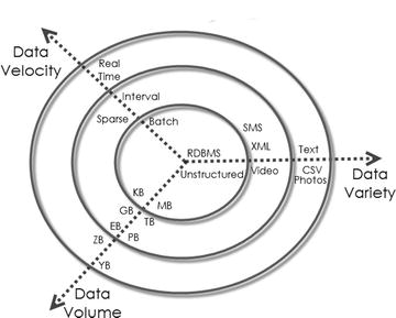
Figure 2-5. 3 V’s of Big data (source: http://blog.sqlauthority.com )
Big data revolution influenced the birth of the term “data science.” Although the term “data science” came into existence from 1960 on, it became popular and this is attributed to Jeff Hammerbacher and DJ Patil, of Facebook and LinkedIn because they carefully chose it, attempting to describe their teams and work (as per Building Data Science Teams by DJ Patil published in 2008); they settled on “data scientist” and a buzzword was born. One picture explains well the essential skills set for data science that was presented by Drew Conway in 2010. See Figure 2-6.
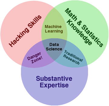
Figure 2-6. Drew Conway’s Data Science Venn diagram
Executing data science projects require three key skills:
Programming or hacking skills,
Math & Statistics,
Business or subject matter expertise for a given area of scope.
Note that the Machine Learning is originated from Artificial Intelligence. It is not a branch of Data science, rather it is only using Machine Learning as a tool.
Statistics vs. Data Mining vs. Data Analytics vs. Data Science
We can learn from the history and evolution of subjects around learning from ‘Data’ is that even though they use the same methods, they evolved as different cultures, so they have different histories, nomenclature, notation, and philosophical perspectives. See Figure 2-7.
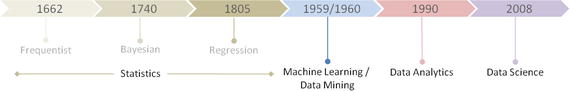
Figure 2-7. Learn from ‘Data’ evolution
All form together to create the path to ultimate Artificial Intelligence. See Figure 2-8.
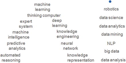
Figure 2-8. All forms together, the path to ultimate Artificial Intelligence
Machine Learning Categories
At a high level, Machine learning tasks can be categorized into three groups based on the desired output and the kind of input required to produce it. See Figure 2-9.
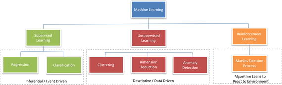
Figure 2-9. Types of Machine Learning
Supervised Learning
The machine learning algorithm is provided with a large enough example input dataset respective output or event/class, usually prepared in consultation with the subject matter expert of a respective domain. The goal of the algorithm is to learn patterns in the data and build a general set of rules to map input to the class or event.
Broadly, there are two types commonly used as supervised learning algorithms .
1) Regression
The output to be predicted is a continuous number in relevance with a given input dataset. Example use cases are predictions of retail sales, prediction of number of staff required for each shift, number of car parking spaces required for a retail store, credit score, for a customer, etc.
2) Classification
The output to be predicted is the actual or the probability of an event/class and the number of classes to be predicted can be two or more. The algorithm should learn the patterns in the relevant input of each class from historical data and be able to predict the unseen class or event in the future considering their input. An example use case is spam email filtering where the output expected is to classify an email into either a “spam” or “not spam.”
Building supervised learning machine learning models has three stages:
Training: The algorithm will be provided with historical input data with the mapped output. The algorithm will learn the patterns within the input data for each output and represent that as a statistical equation, which is also commonly known as a model.
Testing or validation: In this phase the performance of the trained model is evaluated, usually by applying it on a dataset (that was not used as part of the training) to predict the class or event.
Prediction: Here we apply the trained model to a data set that was not part of either the training or testing. The prediction will be used to drive business decisions.
Unsupervised Learning
There are situations where the desired output class/event is unknown for historical data. The objective in such cases would be to study the patterns in the input dataset to get better understanding and identify similar patterns that can be grouped into specific classes or events. As these types of algorithms do not require any intervention from the subject matter experts beforehand, they are called unsupervised learning.
Let’s look at some examples of unsupervised learning .
Clustering
Assume that the classes are not known beforehand for a given dataset. The goal here is to divide the input dataset into logical groups of related items. Some examples are grouping similar news articles, grouping similar customers based on their profile, etc.
Dimension Reduction
Here the goal is to simplify a large input dataset by mapping them to a lower dimensional space. For example, carrying analysis on a large dimension dataset is very computational intensive, so to simplify you may want to find the key variables that hold a significant percentage (say 95%) of information and only use them for analysis.
Anomaly Detection
Anomaly detection is also commonly known as outlier detection is the identification of items, events or observations which do not conform to an expected pattern or behavior in comparison with other items in a given dataset. It has applicability in a variety of domains, such as machine or system health monitoring, event detection, fraud/intrusion detection etc. In the recent days, anomaly detection has seen a big area of interest in the word of Internet of Things (IoT) to enable detection of abnormal behavior in a given context. A data point is termed anomaly if it is distant from other data points in a given context, so calculating standard deviation or clustering are the most commonly used techniques for detection of anomaly alongside a whole lot of other techniques. I’ll not be covering the topic in this edition.
Reinforcement Learning
The basic objective of reinforcement learning algorithms is to map situations to actions that yield the maximum final reward. While mapping the action, the algorithm should not just consider the immediate reward but also next and all subsequent rewards. For example, a program to play a game or drive a car will have to constantly interact with a dynamic environment in which it is expected to perform a certain goal. We’ll learn the basics of Markov decision process/q-learning with an example in a later chapter.
Examples of reinforcement learning techniques are the following:
Markov decision process
Q-learning
Temporal Difference methods
Monte-Carlo methods
Frameworks for Building Machine Learning Systems
Over time data mining field has seen a massive expansion. There have been a lot of efforts taken by many experts to standardize methodologies and define best practice for the ever-growing, diversified, and iterative process of building machine learning systems. On top of the last decade the field of machine learning has become very important for different industries, businesses, and organizations because of its ability to extract insight from huge amounts of data that had previously no use or was underutilized to learn the trend/patterns and predict the possibilities that help to drive business decisions leading to profit. Ultimately the risk of wasting the wealthy and valuable information contained by the rich business data sources was raised, and this required the use of adequate techniques to get useful knowledge so that the field of machine learning had emerged in the early 1980s, it and has seen a great growth. With the emergence of this field, different process frameworks were introduced. These process frameworks guide and carry the machine learning tasks and its applications. Efforts were made to use data mining process frameworks that will guide the implementation of data mining on big or huge amount of data.
Mainly three data mining process frameworks have been most popular, and widely practiced by data mining experts/researchers to build machine learning systems. These models are the following:
Knowledge Discovery Databases (KDD) process model
CRoss Industrial Standard Process for Data Mining (CRISP – DM)
Sample, Explore, Modify, Model and Assess (SEMMA)
Knowledge Discovery Databases (KDD)
This refers to the overall process of discovering useful knowledge from data, which was presented by a book by Fayyad et al., 1996. It is an integration of multiple technologies for data management such as data warehousing, statistic machine learning, decision support, visualization, and parallel computing. As the name suggests, Knowledge Discovery Databases center around the overall process of knowledge discovery from data that covers the entire life cycle of data that includes how the data are stored, how it is accessed, how algorithms can be scaled to enormous datasets efficiently, how results can be interpreted and visualized.
There are five stages in KDD , presented in Figure 2-10.
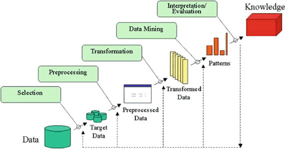
Figure 2-10. KDD Data Mining process flow
Selection
In this step, selection and integration of the target data from possibly many different and heterogeneous sources is performed. Then the correct subset of variables and data samples relevant to the analysis task is retrieved from the database.
Preprocessing
Real-world datasets are often incomplete that is, attribute values will be missing; noisy (errors and outliers); and inconsistent, which means there exists discrepancies between the collected data. The unclean data can confuse the mining procedures and lead to unreliable and invalid outputs. Also, performing complex analysis and mining on a huge amount of such soiled data may take a very long time. Preprocessing and cleaning should improve the quality of data and mining results by enhancing the actual mining process. The actions to be taken include the following:
Collecting required data or information to model
Outlier treatment or removal of noise
Using prior domain knowledge to remove the inconsistencies and duplicates from the data
Choice of strategies for handling missing data
Transformation
In this step, data is transformed or consolidated into forms appropriate for mining, that is, finding useful features to represent the data depending on the goal of the task. For example, in high-dimensional spaces or the large number of attributes, the distances between objects may become meaningless. So dimensionality reduction and transformation methods can be used to reduce the effective number of variables under consideration or find invariant representations for the data. There are various data transformation techniques :
Smoothing (binning, clustering, regression, etc.)
Aggregation
Generalization in which a primitive data object can be replaced by higher-level concepts
Normalization, which involves min-max-scaling or z-score
Feature construction from the existing attributes (PCA, MDS)
Data reduction techniques are applied to produce reduced representation of the data (smaller volume that closely maintains the integrity of the original data)
Compression, for example, wavelets, PCA, clustering etc.
Data Mining
In this step, machine learning algorithms are applied to extract data patterns. Exploration/summarization methods such as mean, median, mode, standard deviation, class/concept description, and graphical techniques of low-dimensional plots can be used to understand the data. Predictive models such as classification or regression can be used to predict the event or future value. Cluster analysis can be used to understand the existence of similar groups. Select the most appropriate methods to be used for the model and pattern search.
Interpretation / Evaluation
This step is focused on interpreting the mined patterns to make them understandable by the user, such as summarization and visualization. The mined pattern or models are interpreted. Patterns are a local structure that makes statements only about restricted regions of the space spanned by the variables. Whereas models are global structures that makes statements about any point in measurement space, that is, Y = mX+C (linear model).
Cross-Industry Standard Process for Data Mining
It is generally known by its acronym CRISP-DM . It was established by the European Strategic Program on Research in Information Technology initiative with an aim to create an unbiased methodology that is not domain dependent. It is an effort to consolidate data mining process best practices followed by experts to tackle data mining problems. It was conceived in 1996 and first published in 1999 and was reported as the leading methodology for data mining/predictive analytics projects in polls conducted in 2002, 2004, and 2007. There was a plan between 2006 and 2008 to update CRISP-DM but that update did not take place, and today the original CRISP-DM.org website is no longer active.
This framework is an idealized sequence of activities. It is an iterative process and many of the tasks backtrack to previous tasks and repeat certain actions to bring more clarity. There are six major phases as shown in Figure 2-11.
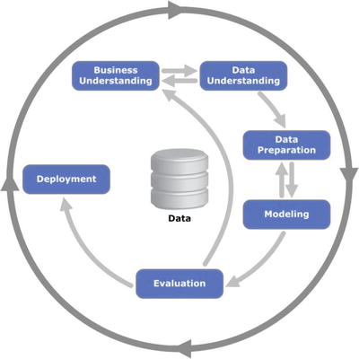
Figure 2-11. Process diagram showing the relationship between the six phases of CRISP-DM
Phase 1: Business Understanding
As the name suggests the focus at this stage is to understand the overall project objectives and expectations from a business perspective. These objectives are converted to a data mining or machine learning problem definition and a plan of action around data requirements, business owners input, and how outcome performance evaluation metrics are designed.
Phase 2: Data Understanding
In this phase, initial data are collected that were identified as requirements in the previous phase. Activities are carried out to understanding data gaps or relevance of the data to the objective in hand, any data quality issues, and first insights into the data to bring out appropriate hypotheses. The outcome of this phase will be presented to the business iteratively to bring more clarity into the business understanding and project objective.
Phase 3: Data Preparation
This phase is all about cleaning the data so that it’s ready to be used for the model building phase. Cleaning data could involve filling the known data gaps from previous steps, missing value treatments, identifying the important features, applying transformations, and creating new relevant features where applicable. This is one of the most important phases as the model’s accuracy will depend significantly on the quality of data that is being fed into the algorithm to learn the patterns.
Phase 4: Modeling
There are multiple machine learning algorithms available to solve a given problem. So various appropriate machine learning algorithms are applied onto the clean dataset, and their parameters are tuned to the optimal possible values. Model performance for each of the applied models is recorded.
Phase 5: Evaluation
In this stage a benchmarking exercise will be carried out among all the different models that were identified to have been giving high accuracy. Model will be tested against data that was not used as part of the training to evaluate its performance consistency. The results will be verified against the business requirement identified in phase 1. The subject matter experts from the business will be involved to ensure that the model results are accurate and usable as per required by the project objective.
Phase 6: Deployment
The key focus in this phase is the usability of the model output. So the final model signed off by the subject matter expert will be implemented, and the consumers of the model output will be trained on how to interpret or use it to take the business decisions defined in the business understanding phase. The implementation could be as generating a prediction report and sharing it with the user. Also periodic model training and prediction times will be scheduled based on the business requirement.
SEMMA (Sample, Explore, Modify, Model, Assess)
SEMMA are the sequential steps to build machine learning models incorporated in ‘SAS Enterprise Miner’, a product by SAS Institute Inc., one of the largest producers of commercial statistical and business intelligence software. However the sequential steps guide the development of a machine learning system. Let’s look at the five sequential steps to understand it better.
Sample
This step is all about selecting the subset of the right volume dataset from a large dataset provided for building the model. This will help us to build the model efficiently. This was a famous practice when the computation power was expensive, however it is still in practice. The selected subset of data should be actual an representation of the entire dataset originally collected, which means it should contain sufficient information to retrieve. The data is also divided for training and validation at this stage.
Explore
In this phase activities are carried out to understand the data gaps and relationship with each other. Two key activities are univariate and multivariate analysis. In univariate analysis each variable looks individually to understand its distribution, whereas in multivariate analysis the relationship between each variable is explored. Data visualization is heavily used to help understand the data better.
Modify
In this phase variables are cleaned where required. New derived features are created by applying business logic to existing features based on the requirement. Variables are transformed if necessary. The outcome of this phase is a clean dataset that can be passed to the machine learning algorithm to build the model.
Model
In this phase, various modeling or data mining techniques are applied on the preprocessed data to benchmark their performance against desired outcomes.
Assess
This is the last phase. Here model performance is evaluated against the test data (not used in model training) to ensure reliability and business usefulness.
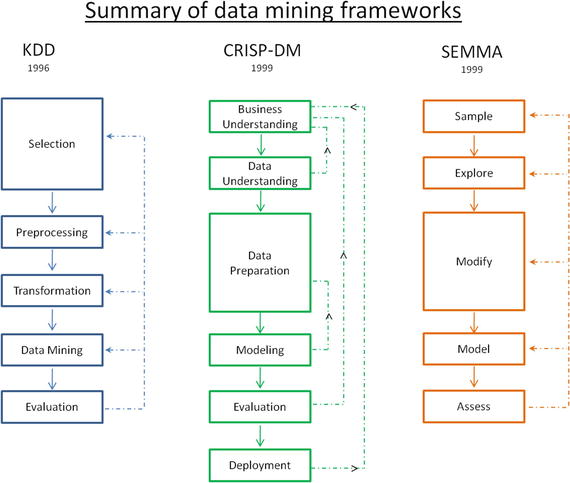
Figure 2-12. Summary of data mining frameworks
KDD vs. CRISP-DM vs. SEMMA
KDD is the oldest of three frameworks. CRISP-DM and SEMMA seem to be the practical implementation of the KDD process. CRISP-DM is more complete as the iterative flow of the knowledge across and between phases has been clearly defined. Also it covers all areas of building a reliable machine learning systems from a business-world perspective. In SEMMA’s sample stage it’s important that you have a true understanding of all aspects of business to ensure the sampled data retains maximum information. However the drastic innovation in the recent past has led to reduced costs for data storage and computational power, which enables us to apply machine learning algorithms on the entire data efficiently, almost removing the need for sampling.
We can see that generally the core phases are covered by all three frameworks and there is not a huge difference between these frameworks. Overall these processes guide us about how data mining techniques can be applied into practical scenarios. In general most of the researchers and data mining experts follow the KDD and CRISP-DM process model because it is more complete and accurate. I personally recommend following CRISP-DM for usage in business environment as it provides coverage of end-to-end business activity and the life cycle of building a machine learning system.
Machine Learning Python Packages
There is a rich number of open source libraries available to facilitate practical machine learning. These are mainly known as scientific Python libraries and are generally put to use when performing elementary machine learning tasks. At a high level we can divide these libraries into data analysis and core machine learning libraries based on their usage/purpose.
Data analysis packages: These are the sets of packages that provide us the mathematic and scientific functionalities that are essential to perform data preprocessing and transformation.
Core Machine learning packages: These are the set of packages that provide us with all the necessary machine learning algorithms and functionalities that can be applied on a given dataset to extract the patterns.
Data Analysis Packages
There are four key packages that are most widely used for data analysis .
NumPy
SciPy
Matplotlib
Pandas
Pandas, NumPy, and Matplotlib play a major role and have the scope of usage in almost all data analysis tasks. So in this chapter we’ll focus on covering usage or concepts relevant to these three packages as much as possible. Whereas SciPy supplements NumPy library and has a variety of key high-level science and engineering modules, the usage of these functions, however, largely depend on the use case to use case. So we’ll touch on or highlight some of the useful functionalities in upcoming chapters where possible. See Figure 2-13.
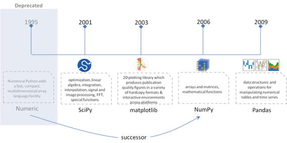
Figure 2-13. Data analysis packages
Note
For conciseness we’ll only be covering the key concepts within each of the libraries with a brief introduction and code implementation. You can always refer to the official user documents for these packages that have been well designed by the developer community to cover a lot more in depth.
NumPy
NumPy is the core library for scientific computing in Python. It provides a high-performance multidimensional array object, and tools for working with these arrays. It’s a successor of Numeric package. In 2005, Travis Oliphant created NumPy by incorporating features of the competing Numarray into Numeric, with extensive modifications. I think the concepts and the code examples to a great extent have been explained in the simplest form in his book Guide to NumPy. Here we’ll only be looking at some of the key NumPy concepts that are a must or good to know in relevance to machine learning.
Array
A NumPy array is a collection of similar data type values, and is indexed by a tuple of nonnegative numbers. The rank of the array is the number of dimensions, and the shape of an array is a tuple of numbers giving the size of the array along each dimension.
We can initialize NumPy arrays from nested Python lists, and access elements using square brackets. See Listing 2-1.
Listing 2-1. Example code for initializing NumPy array
import numpy as np# Create a rank 1 arraya = np.array([0, 1, 2])print type(a)# this will print the dimension of the arrayprint a.shapeprint a[0]print a[1]print a[2]# Change an element of the arraya[0] = 5print a# ----output-----# <type 'numpy.ndarray'># (3L,)# 1# 2# 3# [5 2 3]# Create a rank 2 arrayb = np.array([[0,1,2],[3,4,5]])print b.shapeprint bprint b[0, 0], b[0, 1], b[1, 0]# ----output-----# (2L, 3L)# [[1 2 3]# [4 5 6]]# 1 2 4
Creating NumPy Array
NumPy also provides many built-in functions to create arrays. The best way to learn this is through examples, so let’s jump into the code. See Listing 2-2.
Listing 2-2. Creating NumPy array
# Create a 3x3 array of all zerosa = np.zeros((3,3))print a----- output -----[[ 0. 0. 0.][ 0. 0. 0.][ 0. 0. 0.]]# Create a 2x2 array of all onesb = np.ones((2,2))print b---- output ----[[ 1. 1.][ 1. 1.]]# Create a 3x3 constant arrayc = np.full((3,3), 7)print c---- output ----[[ 7. 7. 7.][ 7. 7. 7.][ 7. 7. 7.]]# Create a 3x3 array filled with random valuesd = np.random.random((3,3))print d---- output ----[[ 0.85536712 0.14369497 0.46311367][ 0.78952054 0.43537586 0.48996107][ 0.1963929 0.12326955 0.00923631]]# Create a 3x3 identity matrixe = np.eye(3)print e---- output ----[[ 1. 0. 0.][ 0. 1. 0.][ 0. 0. 1.]]# convert list to arrayf = np.array([2, 3, 1, 0])print f---- output ----[2 3 1 0]# arange() will create arrays with regularly incrementing valuesg = np.arange(20)print g---- output ----[ 0 1 2 3 4 5 6 7 8 9 10 11 12 13 14 15 16 17 18 19]# note mix of tuple and listsh = np.array([[0, 1,2.0],[0,0,0],(1+1j,3.,2.)])print h---- output ----[[ 0.+0.j 1.+0.j 2.+0.j][ 0.+0.j 0.+0.j 0.+0.j][ 1.+1.j 3.+0.j 2.+0.j]]# create an array of range with float data typei = np.arange(1, 8, dtype=np.float)print i---- output ----[ 1. 2. 3. 4. 5. 6. 7.]# linspace() will create arrays with a specified number of items which are# spaced equally between the specified beginning and end valuesj = np.linspace(2., 4., 5)print j---- output ----[ 2. 2.5 3. 3.5 4. ]# indices() will create a set of arrays stacked as a one-higher# dimensioned array, one per dimension with each representing variation# in that dimensionk = np.indices((2,2))print k---- output ----[[[0 0][1 1]][[0 1][0 1]]]
Data Types
An array is a collection of items of the same data type and NumPy supports and provides built-in functions to construct arrays with optional arguments to explicitly specify required datatypes.
Listing 2-3. NumPy datatypes
# Let numpy choose the datatypex = np.array([0, 1])y = np.array([2.0, 3.0])# Force a particular datatypez = np.array([5, 6], dtype=np.int64)print x.dtype, y.dtype, z.dtype---- output ----int32 float64 int64
Array Indexing
NumPy offers several ways to index into arrays. Standard Python x[obj] syntax can be used to index NumPy array, where x is the array and obj is the selection.
There are three kinds of indexing available:
Field access
Basic slicing
Advanced indexing
Field Access
If the ndarray object is a structured array, the fields of the array can be accessed by indexing the array with strings, dictionary like. Indexing x[‘field-name’] returns a new view to the array, which is of the same shape as x, except when the field is a subarray, but of data type x.dtype[‘field-name’] and contains only the part of the data in the specified field. See Listing 2-4.
Listing 2-4. Field access
x = np.zeros((3,3), dtype=[('a', np.int32), ('b', np.float64, (3,3))])print "x['a'].shape: ",x['a'].shapeprint "x['a'].dtype: ", x['a'].dtypeprint "x['b'].shape: ", x['b'].shapeprint "x['b'].dtype: ", x['b'].dtype# ----output-----# x['a'].shape: (2L, 2L)# x['a'].dtype: int32# x['b'].shape: (2L, 2L, 3L, 3L)# x['b'].dtype: float64
Basic Slicing
NumPy arrays can be sliced, similar to lists. You must specify a slice for each dimension of the array as the arrays may be multidimensional.
The basic slice syntax is i: j: k, where i is the starting index, j is the stopping index, and k is the step and k is not equal to 0. This selects the m elements in the corresponding dimension, with index values i, i + k, …,i + (m - 1) k where m = q + (r not equal to 0) and q and r are the quotient and the remainder is obtained by dividing j - i by k: j - i = q k + r, so that i + (m - 1) k < j. See Listing 2-5.
Listing 2-5. Basic slicing
x = np.array([5, 6, 7, 8, 9])x[1:7:2]---- output ----array([6, 8])Negative k makes stepping go toward smaller indices. Negative i and j are interpreted as n + i and n + j where n is the number of elements in the corresponding dimension.print x[-2:5]print x[-1:1:-1]# ---- output ----[8 9][9 8 7]If n is the number of items in the dimension being sliced. Then if i is not given then it defaults to 0 for k > 0 and n - 1 for k < 0. If j is not given it defaults to n for k > 0 and -1 for k < 0. If k is not given it defaults to 1. Note that :: is the same as : and means select all indices along this axis.x[4:]# ---- output ----array([9])If the number of objects in the selection tuple is less than N, then : is assumed for any subsequent dimensions.
Listing 2-6. Basic slicing
y = np.array([[[1],[2],[3]], [[4],[5],[6]]])print "Shape of y: ", x.shapey[1:3]# ---- output ----Shape of y: (3L)array([[[4], [5], [6]], [7]], dtype=object)Ellipsis expand to the number of : objects needed to make a selection tuple of the same length as x.ndim. There may only be a single ellipsis present.x[...,0]---- output ----array([[0], [1], [2], [3]], dtype=object)# Create a rank 2 array with shape (3, 4)a = np.array([[5,6,7,8], [1,2,3,4], [9,10,11,12]])print "Array a:", a# Use slicing to pull out the subarray consisting of the first 2 rows# and columns 1 and 2; b is the following array of shape (2, 2):# [[2 3]# [6 7]]b = a[:2, 1:3]print "Array b:", b---- output ----Array a: [[ 5 6 7 8][ 1 2 3 4][ 9 10 11 12]]Array b: [[6 7][2 3]]A slice of an array is a view into the same data, so modifying itwill modify the original array.print a[0, 1]b[0, 0] = 77print a[0, 1]# ---- output ----# 6# 77.Middle row array can be accessed in two ways. 1) Slices along with integer indexing will result in an arry of lower rank. 2) Using only slices will result in same rank array.Example code:row_r1 = a[1,:]# Rank 1 view of the second row of arow_r2 = a[1:2,:]# Rank 2 view of the second row of aprint row_r1, row_r1.shape # Prints "[5 6 7 8] (4,)"print row_r2, row_r2.shape # Prints "[[5 6 7 8]] (1, 4)"---- output ----[1 2 3 4] (4L,)[[1 2 3 4]] (1L, 4L)[[1 2 3 4]] (1L, 4L)# We can make the same distinction when accessing columns of an array:col_r1 = a[:, 1]col_r2 = a[:, 1:2]print col_r1, col_r1.shape # Prints "[ 2 6 10] (3,)"print col_r2, col_r2.shape---- output ----[77 2 10] (3L,)[[77][ 2][10]] (3L, 1L)
Advanced Indexing
Integer array indexing : Integer array indexing allows you to construct random arrays and other arrays. See Listing 2-7.
Listing 2-7. Advanced indexinga = np.array([[1,2], [3, 4]])
# An example of integer array indexing.# The returned array will have shape (2,) andprint a[[0, 1], [0, 1]]# The above example of integer array indexing is equivalent to this:print np.array([a[0, 0], a[1, 1]]) --- output ----[1 4][1 4]# When using integer array indexing, you can reuse the same# element from the source array:print a[[0, 0], [1, 1]]# Equivalent to the previous integer array indexing exampleprint np.array([a[0, 1], a[0, 1]])---- output ----[2 2][2 2]
Boolean array indexing: This is useful to pick a random element from an array, which is often used for filtering elements that satisfy a given condition. See Listing 2-8.
Listing 2-8. Boolean array indexing
a=np.array([[1,2], [3, 4], [5, 6]])# Find the elements of a that are bigger than 2print (a > 2)# to get the actual valueprint a[a > 2]---- output ----[[False False][ True True][ True True]][3 4 5 6]
Array Math
Basic mathematical functions are available as operators and also as functions in NumPy. It operates element-wise on an array. See Listing 2-9.
Listing 2-9. Array math
import numpy as npx=np.array([[1,2],[3,4],[5,6]])y=np.array([[7,8],[9,10],[11,12])# Elementwise sum; both produce the arrayprintx+yprintnp.add(x, y)# ---- output ----[[ 8 10][12 14][16 18]][[ 8 10][12 14][16 18]]# Elementwise difference; both produce the arrayprintx-yprintnp.subtract(x, y)# ---- output ----[[-4. -4.][-4. -4.]][[-4. -4.][-4. -4.]]# Elementwise product; both produce the arrayprintx*yprintnp.multiply(x, y)# ---- output ----[[ 5. 12.][ 21. 32.]][[ 5. 12.][ 21. 32.]]# Elementwise division; both produce the arrayprintx/yprintnp.divide(x, y)# ---- output ----[[ 0.2 0.33333333][ 0.42857143 0.5 ]][[ 0.2 0.33333333][ 0.42857143 0.5 ]]# Elementwise square root; produces the arrayprintnp.sqrt(x)# ---- output ----[[ 1. 1.41421356][ 1.73205081 2.]]
We can use the “dot” function to calculate inner products of vectors or to multiply matrices or multiply a vector by a matrix. See Listing 2-10.
Listing 2-10. Array math (continued)
x=np.array([[1,2],[3,4]])y=np.array([[5,6],[7,8]])a=np.array([9,10])b=np.array([11, 12])# Inner product of vectors; both produce 219Printa.dot(b)Printnp.dot(a, b)# ---- output ----219219# Matrix / vector product; both produce the rank 1 array [29 67]Printx.dot(a)Printnp.dot(x, a)# ---- output ----[29 67][29 67]# Matrix / matrix product; both produce the rank 2 arrayprintx.dot(y)printnp.dot(x, y)# ---- output ----[[19 22][43 50]][[19 22][43 50]]
NumPy provides many useful functions for performing computations on arrays. One of the most useful is sum. See Listing 2-11.
Listing 2-11. Sum function
x=np.array([[1,2],[3,4]])# Compute sum of all elementsprint np.sum(x)# Compute sum of each columnprint np.sum(x, axis=0)# Compute sum of each rowprint np.sum(x, axis=1)# ---- output ----10[4 6][3 7]
Transpose is one of the common operations often performed on matrix, which can be achieved using the T attribute of an array object. See Listing 2-12.
Listing 2-12. Transpose function
x=np.array([[1,2], [3,4]])printxprintx.T# ---- output ----[[1 2][3 4]][[1 3][2 4]]# Note that taking the transpose of a rank 1 array does nothing:v=np.array([1,2,3])printvprintv.T# ---- output ----[1 2 3][1 2 3]
Broadcasting
Broadcasting enables arithmetic operations to be performed between different shaped arrays. Let’s look at a simple example of adding a constant vector to each row of a matrix. See Listing 2-13.
Listing 2-13. Broadcasting
# create a matrixa = np.array([[1,2,3], [4,5,6], [7,8,9]])# create a vectorv = np.array([1, 0, 1])# create an empty matrix with the same shape as ab = np.empty_like(a)# Add the vector v to each row of the matrix x with an explicit loopfor i in range(3):b[i, :] = a[i, :] + vprint b# ---- output ----[[ 2 2 4][ 5 5 7][ 8 8 10]]
If you have to perform the above operation on a large matrix, the through loop in Python could be slow. Let’s look at an alternative approach. See Listing 2-14.
Listing 2-14. Broadcasting for large matrix
# Stack 3 copies of v on top of each othervv = np.tile(v, (3, 1))print vv# ---- output ----[[1 0 1][1 0 1][1 0 1]]# Add a and vv elementwiseb = a + vvprint b# ---- output ----[[ 2 2 4][ 5 5 7][ 8 8 10]]
Now let’s see in Listing 2-15 how the above can be achieved using NumPy broadcasting.
Listing 2-15. Broadcasting using NumPy
a = np.array([[1,2,3], [4,5,6], [7,8,9]])v = np.array([1, 0, 1])# Add v to each row of a using broadcastingb = a + vprint b# ---- output ----[[ 2 2 4][ 5 5 7][ 8 8 10]]
Now let’s look at some applications of broadcasting in Listing 2-16.
Listing 2-16. Applications of broadcasting
# Compute outer product of vectors# v has shape (3,)v = np.array([1,2,3])# w has shape (2,)w = np.array([4,5])# To compute an outer product, we first reshape v to be a column# vector of shape (3, 1); we can then broadcast it against w to yield# an output of shape (3, 2), which is the outer product of v and w:print np.reshape(v, (3, 1)) * w# ---- output ----[[ 4 5][ 8 10][12 15]]# Add a vector to each row of a matrixx = np.array([[1,2,3],[4,5,6]])# x has shape (2, 3) and v has shape (3,) so they broadcast to (2, 3)printx + v# ---- output ----[[2 4 6][5 7 9]]# Add a vector to each column of a matrix# x has shape (2, 3) and w has shape (2,).# If we transpose x then it has shape (3, 2) and can be broadcast# against w to yield a result of shape (3, 2); transposing this result# yields the final result of shape (2, 3) which is the matrix x with# the vector w added to each columnprint(x.T + w).T# ---- output ----[[ 5 6 7][ 9 10 11]]# Another solution is to reshape w to be a row vector of shape (2, 1);# we can then broadcast it directly against x to produce the same# output.printx + np.reshape(w,(2,1))# ---- output ----[[ 5 6 7][ 9 10 11]]# Multiply a matrix by a constant:# x has shape (2, 3). Numpy treats scalars as arrays of shape ();# these can be broadcast together to shape (2, 3)printx * 2# ---- output ----[[ 2 4 6][ 8 10 12]]
Broadcasting typically makes your code more concise and faster, so you should strive to use it where possible.
Pandas
Python has always been great for data munging; however it was not great for analysis compared to databases using SQL or Excel or R data frames . Pandas are an open source Python package providing fast, flexible, and expressive data structures designed to make working with “relational” or “labeled” data both easy and intuitive. Pandas were developed by Wes McKinney in 2008 while at AQR Capital Management out of the need for a high performance, flexible tool to perform quantitative analysis on financial data. Before leaving AQR he was able to convince management to allow him to open source the library.
Pandas are well suited for tabular data with heterogeneously typed columns, as in an SQL table or Excel spreadsheet.
Data Structures
Pandas introduces two new data structures to Python – Series and DataFrame, both of which are built on top of NumPy (this means it’s fast).
Series
This is a one-dimensional object similar to column in a spreadsheet or SQL table. By default each item will be assigned an index label from 0 to N. See Listing 2-17.
Listing 2-17. Creating a pandas series
# creating a series by passing a list of values, and a custom index label. Note that the labeled index reference for each row and it can have duplicate valuess = pd.Series([1,2,3,np.nan,5,6], index=['A','B','C','D','E','F'])print s# ---- output ----# A 1.0# B 2.0# C 3.0# D NaN# E 5.0# F 6.0# dtype: float64
DataFrame
It is a two-dimensional object similar to a spreadsheet or an SQL table. This is the most commonly used pandas object. See Listing 2-18.
Listing 2-18. Creating a pandas dataframe
data = {'Gender': ['F', 'M', 'M'],'Emp_ID': ['E01', 'E02', 'E03'], 'Age': [25, 27, 25]}# We want the order the columns, so lets specify in columns parameterdf = pd.DataFrame(data, columns=['Emp_ID','Gender', 'Age'])df# ---- output ----# Emp_ID Gender Age#0 E01 F 25#1 E02 M 27#2 E03 M 25
Reading and Writing Data
We’ll see three commonly used file formats: csv, text file, and Excel in Listing 2-19.
Listing 2-19. Reading / writing data from csv, text, Excel
# Readingdf=pd.read_csv('Data/mtcars.csv') # from csvdf=pd.read_csv('Data/mtcars.txt', sep=' ') # from text filedf=pd.read_excel('Data/mtcars.xlsx','Sheet2') # from Excel# reading from multiple sheets of same Excel into different dataframesxlsx = pd.ExcelFile('file_name.xls')sheet1_df = pd.read_excel(xlsx, 'Sheet1')sheet2_df = pd.read_excel(xlsx, 'Sheet2')# writing# index = False parameter will not write the index values, default is Truedf.to_csv('Data/mtcars_new.csv', index=False)df.to_csv('Data/mtcars_new.txt', sep=' ', index=False)df.to_excel('Data/mtcars_new.xlsx',sheet_name='Sheet1', index = False)
Note
Write will by default overwrite any existing file with the same name.
Basic Statistics Summary
Pandas has some built-in functions to help us to get better understanding of data using basic statistical summary methods. See Listings 2-20, 2-21, and 2-22.
describe()- will returns the quick stats such as count, mean, std (standard deviation), min, first quartile, median, third quartile, max on each column of the dataframeListing 2-20. Basic statistics on dataframe
df = pd.read_csv('Data/iris.csv')df.describe()#---- output ----#Sepal.Length Sepal.Width Petal.Length Petal.Width#count 150.000000 150.000000 150.000000 150.000000#mean 5.843333 3.057333 3.758000 1.199333#std 0.828066 0.435866 1.765298 0.762238#min 4.300000 2.000000 1.000000 0.100000#25% 5.100000 2.800000 1.600000 0.300000#50% 5.800000 3.000000 4.350000 1.300000#75% 6.400000 3.300000 5.100000 1.800000#max 7.900000 4.400000 6.900000 2.500000cov() - Covariance indicates how two variables are related. A positive covariance means the variables are positively related, while a negative covariance means the variables are inversely related. Drawback of covariance is that it does not tell you the degree of positive or negative relation
Listing 2-21. Creating covariance on dataframe
df = pd.read_csv('Data/iris.csv')df.cov()#---- output ----#Sepal.Length Sepal.Width Petal.Length Petal.Width#Sepal.Length 0.685694 -0.042434 1.274315 0.516271#Sepal.Width -0.042434 0.189979 -0.329656 -0.121639#Petal.Length 1.274315 -0.329656 3.116278 1.295609#Petal.Width 0.516271 -0.121639 1.295609 0.581006corr() - Correlation is another way to determine how two variables are related. In addition to telling you whether variables are positively or inversely related, correlation also tells you the degree to which the variables tend to move together. When you say that two items correlate, you are saying that the change in one item effects a change in another item. You will always talk about correlation as a range between -1 and 1. In the below example code, petal length is 87% positively related to sepal length that means a change in petal length results in a positive 87% change to sepal lenth and vice versa.
Listing 2-22. Creating correlation matrix on dataframe
df = pd.read_csv('Data/iris.csv')df.corr()#----output----# Sepal.Length Sepal.Width Petal.Length Petal.Width#Sepal.Length 1.000000 -0.117570 0.871754 0.817941#Sepal.Width -0.117570 1.000000 -0.428440 -0.366126#Petal.Length 0.871754 -0.428440 1.000000 0.962865#Petal.Width 0.817941 -0.366126 0.962865 1.000000
Viewing Data
The Pandas dataframe comes with built-in functions to view the contained data. See Table 2-2.
Table 2-2. Pandas view function
Describe | Syntax |
|---|---|
Looking at the top n records default n value is 5 if not specified | df.head(n=2) |
Looking at the bottom n records | df.tail() |
Get column names | df.columns |
Get column datatypes | df.dtypes |
Get dataframe index | df.index |
Get unique values | df[column_name].unique() |
Get values | df.values |
Sort DataFrame | df.sort_values(by =[‘Column1’, ‘Column2’], ascending=[True,True’]) |
select/view by column name | df[column_name] |
select/view by row number | df[0:3] |
selection by index | df.loc[0:3] # index 0 to 3 df.loc[0:3,[‘column1’, ‘column2’]] # index 0 to 3 for specific columns |
selection by position | df.iloc[0:2] # using range, first 2 rows df.iloc[2,3,6] # specific position df.iloc[0:2,0:2] # first 2 rows and first 2 columns |
selection without it being in the index | print df.ix[1,1] # value from fist row and first column print df.ix[:,2] # all rows of column at 2nd position |
Faster alternative to iloc to get scalar values | print df.iat[1,1] |
Transpose DataFrame | df.T |
Filter DataFrame based on value condition for one column | df[df[‘column_name’] > 7.5] |
Filter DataFrame based on a value condition on one column | df[df[‘column_name’].isin([‘condition_value1’, ‘condition_value2’])] |
Filter based on multiple conditions on multiple columns using AND operator | df[(df[‘column1’]>7.5) & (df[‘column2’]>3)] |
Filter based on multiple conditions on multiple columns using OR operator | df[(df[‘column1’]>7.5) | (df[‘column2’]>3)] |
Basic Operations
Pandas comes with a rich set of built-in functions for basic operations. See Table 2-3.
Table 2-3. Pandas basic operations
Description | Syntax |
|---|---|
Convert string to date series | pd.to_datetime(pd.Series([‘2017-04-01’,‘2017-04-02’,‘2017-04-03’])) |
Rename a specific column name | df.rename(columns={‘old_columnname’:‘new_columnname’}, inplace=True) |
Rename all column names of DataFrame | df.columns = [‘col1_new_name’,‘col2_new_name’….] |
Flag duplicates | df.duplicated() |
Drop duplicates | df = df.drop_duplicates() |
Drop duplicates in specific column | df.drop_duplicates([‘column_name’]) |
Drop duplicates in specific column, but retain the first or last observation in duplicate set | df.drop_duplicates([‘column_name’], keep = ‘first’) # change to last for retaining last obs of duplicate |
Creating new column from existing column | df[‘new_column_name’] = df[‘existing_column_name’] + 5 |
Creating new column from elements of two columns | df[‘new_column_name’] = df[‘existing_column1’] + ‘_’ + df[‘existing_column2’] |
Adding a list or a new column to DataFrame | df[‘new_column_name’] = pd.Series(mylist) |
Drop missing rows and columns having missing values | df.dropna() |
Replaces all missing values with 0 (or you can use any int or str) | df.fillna(value=0) |
Replace missing values with last valid observation (useful in time series data). For example, temperature does not change drastically compared to previous observation. So better approach is to fill NA is to forward or backward fill than mean. There are mainly two methods available 1) ‘pad’ / ‘ffill’ - forward fill 2) ‘bfill’ / ‘backfill’ - backward fill
Limit: If method is specified, this is the maximum number of consecutive NaN values to forward/backward fill | df.fillna(method=‘ffill’, inplace=True, limit = 1) |
Check missing value condition and return Boolean value of true or false for each cell | pd.isnull(df) |
Replace all missing values for a given column with its mean | mean=df[‘column_name’].mean(); df[‘column_name’].fillna(mean) |
Return mean for each column | df.mean() |
Return max for each column | df.max() |
Return min for each column | df.min() |
Return sum for each column | df.sum() |
Return count for each column | df.count() |
Return cumulative sum for each column | df.cumsum() |
Applies a function along any axis of the DataFrame | df.apply(np.cumsum) |
Iterate over each element of a series and perform desired action | df[‘column_name’].map(lambda x: 1+x) # this iterates over the column and adds value 1 to each element |
Apply a function to each element of dataframe | func = lambda x: x + 1 # function to add a constant 1 to each element of dataframe df.applymap(func) |
Merge/Join
Pandas provide various facilities for easily combining together Series, DataFrame, and Panel objects with various kinds of set logic for the indexes and relational algebra functionality in the case of join merge-type operations. See Figure 2-27.
Listing 2-23. Concat or append operation
data = {'emp_id': ['1', '2', '3', '4', '5'],'first_name': ['Jason', 'Andy', 'Allen', 'Alice', 'Amy'],'last_name': ['Larkin', 'Jacob', 'A', 'AA', 'Jackson']}df_1 = pd.DataFrame(data, columns = ['emp_id', 'first_name', 'last_name'])data = {'emp_id': ['4', '5', '6', '7'],'first_name': ['Brian', 'Shize', 'Kim', 'Jose'],'last_name': ['Alexander', 'Suma', 'Mike', 'G']}df_2 = pd.DataFrame(data, columns = ['emp_id', 'first_name', 'last_name'])# Usingconcatdf = pd.concat([df_1, df_2])printdf# or# Using appendprint df_1.append(df_2)# Join the two dataframes along columnspd.concat([df_1, df_2], axis=1)# ---- output ----# Table df_1# emp_idfirst_namelast_name#0 1 Jason Larkin#1 2 Andy Jacob#2 3 Allen A#3 4 Alice AA#4 5 Amy Jackson# Table df_2#emp_idfirst_namelast_name#0 4 Brian Alexander#1 5 Shize Suma#2 6 Kim Mike#3 7 Jose G# concated table# emp_idfirst_namelast_name#0 1 Jason Larkin#1 2 Andy Jacob#2 3 Allen A#3 4 Alice AA#4 5 Amy Jackson#0 4 Brian Alexander#1 5 Shize Suma#2 6 Kim Mike#3 7 Jose G# concated along columns#emp_idfirst_namelast_nameemp_idfirst_namelast_name#0 1 Jason Larkin 4 Brian Alexander#1 2 Andy Jacob 5 Shize Suma#2 3 Allen A 6 Kim Mike#3 4 Alice AA 7 Jose G#4 5 Amy Jackson NaNNaNNaN
Merge two dataframes based on a common column as shown in Listing 2-24.
Listing 2-24. Merge two dataframes
# Merge two dataframes based on the emp_id value# in this case only the emp_id's present in both table will be joinedpd.merge(df_1, df_2, on='emp_id')# ---- output ----# emp_id first_name_x last_name_x first_name_y last_name_y#0 4 Alice AA Brian Alexander#1 5 Amy Jackson Shize Suma
Join
Pandas offer SQL style merges as well.
Left join produces a complete set of records from Table A, with the matching records where available in Table B. If there is no match, the right side will contain null.
Note Note that you can suffix to avoid duplicate; if not provided it will automatically add x to the Table A and y to Table B. See Listings 2-25 and 2-26.
Listing 2-25. Left join two dataframes
# Left joinprint pd.merge(df_1, df_2, on='emp_id', how='left')# Merge while adding a suffix to duplicate column names of both tableprint pd.merge(df_1, df_2, on='emp_id', how='left', suffixes=('_left', '_right'))# ---- output ----# ---- without suffix ----# emp_id first_name_x last_name_x first_name_y last_name_y#0 1 Jason Larkin NaN NaN#1 2 Andy Jacob NaN NaN#2 3 Allen A NaN NaN#3 4 Alice AA Brian Alexander#4 5 Amy Jackson Shize Suma# ---- with suffix ----# emp_id first_name_left last_name_left first_name_right last_name_right#0 1 Jason Larkin NaN NaN#1 2 Andy Jacob NaN NaN#2 3 Allen A NaN NaN#3 4 Alice AA Brian Alexander#4 5 Amy Jackson Shize SumaRight join - Right join produces a complete set of records from Table B, with the matching records where available in Table A. If there is no match, the left side will contain null.
Listing 2-26. Right join two dataframes
# Left joinpd.merge(df_1, df_2, on='emp_id', how='right')'# ---- output ----# emp_id first_name_x last_name_x first_name_y last_name_y#0 4 Alice AA Brian Alexander#1 5 Amy Jackson Shize Suma#2 6 NaN NaN Kim Mike#3 7 NaN NaN Jose G
Inner Join - Inner join produces only the set of records that match in both Table A and Table B. See Listing 2-27.
Listing 2-27. Inner join two dataframespd.merge(df_1, df_2, on=‘emp_id’, how=‘inner’)
# ---- output ----# emp_id first_name_x last_name_x first_name_y last_name_y#0 4 Alice AA Brian Alexander#1 5 Amy Jackson Shize Suma
Outer Join - Full outer join produces the set of all records in Table A and Table B, with matching records from both sides where available. If there is no match, the missing side will contain null as in Listing 2-28.
Listing 2-28. Outer join two dataframes
pd.merge(df_1, df_2, on='emp_id', how='outer')# ---- output ----# emp_id first_name_x last_name_x first_name_y last_name_y#0 1 Jason Larkin NaN NaN#1 2 Andy Jacob NaN NaN#2 3 Allen A NaN NaN#3 4 Alice AA Brian Alexander#4 5 Amy Jackson Shize Suma#5 6 NaN NaN Kim Mike#6 7 NaN NaN Jose G
Grouping
Grouping involves one or more of the following steps:
Splitting the data into groups based on some criteria,
Applying a function to each group independently,
Combining the results into a data structure (see Listing 2-29).
Listing 2-29. Grouping operation
df = pd.DataFrame({'Name' : ['jack', 'jane', 'jack', 'jane', 'jack', 'jane', 'jack', 'jane'],'State' : ['SFO', 'SFO', 'NYK', 'CA', 'NYK', 'NYK', 'SFO', 'CA'],'Grade':['A','A','B','A','C','B','C','A'],'Age' : np.random.uniform(24, 50, size=8),'Salary' : np.random.uniform(3000, 5000, size=8),})# Note that the columns are ordered automatically in their alphabetic orderdf# for custom order please use below code# df = pd.DataFrame(data, columns = ['Name', 'State', 'Age','Salary'])# Find max age and salary by Name / State# with groupby, we can use all aggregate functions such as min, max, mean, count, cumsumdf.groupby(['Name','State']).max()# ---- output ----# ---- DataFrame ----# Age Grade Name Salary State#0 45.364742 A jack 3895.416684 SFO#1 48.457585 A jane 4215.666887 SFO#2 47.742285 B jack 4473.734783 NYK#3 35.181925 A jane 4866.492808 CA#4 30.285309 C jack 4874.123001 NYK#5 35.649467 B jane 3689.269083 NYK#6 42.320776 C jack 4317.227558 SFO#7 46.809112 A jane 3327.306419 CA# ----- find max age and salary by Name / State -----# Age Grade Salary#Name State#jack NYK 47.742285 C 4874.123001# SFO 45.364742 C 4317.227558#jane CA 46.809112 A 4866.492808# NYK 35.649467 B 3689.269083# SFO 48.457585 A 4215.666887
Pivot Tables
Pandas provides a function ‘pivot_table’ to create MS-Excel spreadsheet style pivot tables. It can take following arguments:
data: DataFrame object,
values: column to aggregate,
index: row labels,
columns: column labels,
aggfunc: aggregation function to be used on values, default is NumPy.mean (see Listing 2-30).
Listing 2-30. Pivot tables
# by state and name find mean age for each gradepd.pivot_table(df, values='Age', index=['State', 'Name'], columns=['Grade'])# ---- output ----#Grade A B C#State Name#CA jane 40.995519 NaN NaN#NYK jack NaN 47.742285 30.285309# jane NaN 35.649467 NaN#SFO jack 45.364742 NaN 42.320776# jane 48.457585 NaN NaN
Matplotlib
Matplotlib is a numerical mathematics extension NumPy and a great package to view or present data in a pictorial or graphical format. It enables analysts and decision makers to see analytics presented visually, so they can grasp difficult concepts or identify new patterns.
There are two broad ways of using pyplo.
Using Global Functions
The most common and easy approach is by using global functions to build and display a global figure using matplotlib as a global state machine. Let’s look at some of the most commonly used charts. Then see Listing 2-31.
plt.bar – creates a bar chart
plt.scatter – makes a scatter plot
plt.boxplot – makes a box and whisker plot
plt.hist – makes a histogram
plt.plot – creates a line plot
Listing 2-31. Creating plot on variables
# simple bar and scatter plotx = np.arange(5) # assume there are 5 studentsy = (20, 35, 30, 35, 27) # their test scoresplt.bar(x,y) # Bar plot# need to close the figure using show() or close(), if not closed any follow up plot commands will use same figure.plt.show() # Try commenting this an runplt.scatter(x,y) # scatter plotplt.show()# ---- output ----
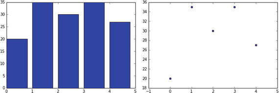
You can use the histogram, line graph, and boxplot directly on a dataframe. You can see that it’s very quick and does not take much coding effort. See Listing 2-32.
Listing 2-32. Creating plot on dataframe df = pd.read_csv(‘Data/iris.csv’) # Read sample data
df.hist()# Histogramdf.plot() # Line Graphdf.boxplot() # Box plot# --- histogram----------line graph ----------box plot-------
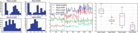
Customizing Labels
You can customize the labels to make them more meaningful. See Listing 2-33.
Listing 2-33. Customize labels
# generate sample datax = np.linspace(0, 20, 1000) #100 evenly-spaced values from 0 to 50y = np.sin(x)# customize axis labelsplt.plot(x, y, label = 'Sample Label')plt.title('Sample Plot Title') # chart titleplt.xlabel('x axis label') # x axis titleplt.ylabel('y axis label') # y axis titleplt.grid(True) # show gridlines# add footnoteplt.figtext(0.995, 0.01, 'Footnote', ha='right', va='bottom')# add legend, location pick the best automaticallyplt.legend(loc='best', framealpha=0.5, prop={'size':'small'})# tight_layout() can take keyword arguments of pad, w_pad and h_pad.# these control the extra padding around the figure border and between subplots.# The pads are specified in fraction of fontsize.plt.tight_layout(pad=1)# Saving chart to a fileplt.savefig('filename.png')plt.close() # Close the current window to allow new plot creation on separate window / axis, alternatively we can use show()plt.show()# ---- output ----
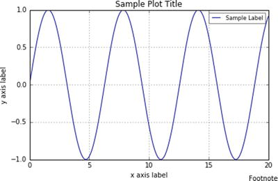
Object Oriented
You obtain an empty figure from a global factory, and then build the plot explicitly using the methods of the Figure and the classes it contains. The Figure is the top-level container for everything on a canvas. Axes is a container class for a specific plot. A figure may contain many Axes and/or Subplots. Subplots are laid out in a grid within the Figure. Axes can be placed anywhere on the Figure. We can use the subplots factory to get the Figure and all the desired Axes at once. See Listing 2-34.
Listing 2-34. Object-oriented customization
fig, ax = plt.subplots()fig,(ax1,ax2,ax3) = plt.subplots(nrows=3, ncols=1, sharex=True, figsize=(8,4))# Iterating the Axes within a Figurefor ax in fig.get_axes():pass # do something# ---- output ----
Line Plots – Using ax.plot()
Single plot constructed with Figure and Axes in Llisting 2-35.
Listing 2-35. Single line plot using ax.plot()
# generate sample datax = np.linspace(0, 20, 1000)y = np.sin(x)fig = plt.figure(figsize=(8,4)) # get an empty figure and add an Axesax = fig.add_subplot(1,1,1) # row-col-numax.plot(x, y, 'b-', linewidth=2, label='Sample label') # line plot data on the Axes# add title, labels and legend, etc.ax.set_ylabel('y axis label', fontsize=16) # y labelax.set_xlabel('x axis lable', fontsize=16) # x labelax.legend(loc='best') # legendax.grid(True) # show gridfig.suptitle('Sample Plot Title') # titlefig.tight_layout(pad=1) # tidy laytoutfig.savefig('filename.png', dpi=125)# ---- output ----
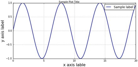
Multiple Lines on Same Axis
See Listing 2-36.
Listing 2-36. Multiple line plot on same axis
# get the Figure and Axes all at oncefig, ax = plt.subplots(figsize=(8,4))x1 = np.linspace(0, 100, 20)x2 = np.linspace(0, 100, 20)x3 = np.linspace(0, 100, 20)y1 = np.sin(x1)y2 = np.cos(x2)y3 = np.tan(x3)ax.plot(x1, y1, label='sin')ax.plot(x2, y2, label='cos')ax.plot(x3, y3, label='tan')# add grid, legend, title and saveax.grid(True)ax.legend(loc='best', prop={'size':'large'})fig.suptitle('A Simple Multi Axis Line Plot')fig.savefig('filename.png', dpi=125)# ---- output ----
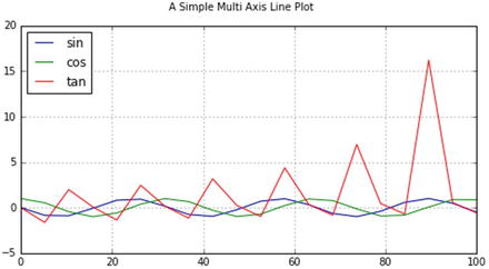
Multiple Lines on Different Axis
See Listing 2-37.
Listing 2-37. Multiple lines on different axis
# Changing sharex to True will use the same x axisfig, (ax1,ax2,ax3) = plt.subplots(nrows=3, ncols=1, sharex=False, sharey = False, figsize=(8,4))# plot some linesx1 = np.linspace(0, 100, 20)x2 = np.linspace(0, 100, 20)x3 = np.linspace(0, 100, 20)y1 = np.sin(x1)y2 = np.cos(x2)y3 = np.tan(x3)ax1.plot(x1, y1, label='sin')ax2.plot(x2, y2, label='cos')ax3.plot(x3, y3, label='tan')# add grid, legend, title and saveax1.grid(True)ax2.grid(True)ax3.grid(True)ax1.legend(loc='best', prop={'size':'large'})ax2.legend(loc='best', prop={'size':'large'})ax3.legend(loc='best', prop={'size':'large'})fig.suptitle('A Simple Multi Axis Line Plot')fig.savefig('filename.png', dpi=125)# ---- output ----
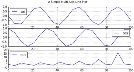
Control the Line Style and Marker Style
See Listing 2-38.
Listing 2-38. Line style and marker style controls
# get the Figure and Axes all at oncefig, ax = plt.subplots(figsize=(8,4))# plot some linesN = 3 # the number of lines we will plotstyles = ['-', '--', '-.', ':']markers = list('+ox')x = np.linspace(0, 100, 20)for i in range(N): # add line-by-liney = x + x/5*i + is = styles[i % len(styles)]m = markers[i % len(markers)]ax.plot(x, y, alpha = 1, label='Line '+str(i+1)+' '+s+m,marker=m, linewidth=2, linestyle=s)# add grid, legend, title and saveax.grid(True)ax.legend(loc='best', prop={'size':'large'})fig.suptitle('A Simple Line Plot')fig.savefig('filename.png', dpi=125)# ---- output ----
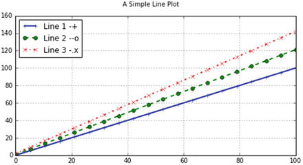

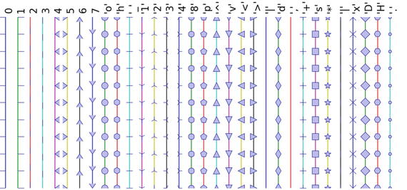
Colomaps Reference
See Figure 2-16.
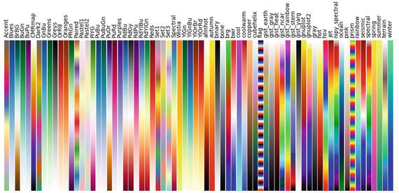
Figure 2-16. Matplotlib colormaps reference
Note
All color maps can be reversed by appending _r. For instance, gray_r is the reverse of gray.
Bar Plots – using ax.bar() and ax.barh()
See Listing 2-39.
Listing 2-39. Bar plots using ax.bar() and ax.barh()
# get the dataN = 4labels = list('ABCD')data = np.array(range(N)) + np.random.rand(N)#plot the datafig, ax = plt.subplots(figsize=(8, 3.5))width = 0.5;tickLocations = np.arange(N)rectLocations = tickLocations-(width/2.0)# for color either HEX value of the name of the color can be usedax.bar(rectLocations, data, width,color='lightblue',edgecolor='#1f10ed', linewidth=4.0)# tidy-up the plotax.set_xticks(ticks= tickLocations)ax.set_xticklabels(labels)ax.set_xlim(min(tickLocations)-0.6, max(tickLocations)+0.6)ax.set_yticks(range(N)[1:])ax.set_ylim((0,N))ax.yaxis.grid(True)ax.set_ylabel('y axis label', fontsize=8) # y labelax.set_xlabel('x axis lable', fontsize=8) # x label# title and savefig.suptitle("Bar Plot")fig.tight_layout(pad=2)fig.savefig('filename.png', dpi=125)# ---- output ----
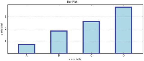
Horizontal Bar Charts
Just as tick placement needs to be managed with vertical bars, so it is with horizontal bars, which are above the y-tick mark as shown in Listing 2-40.
Listing 2-40. Horizontal bar charts
# get the dataN = 4labels = list('ABCD')data = np.array(range(N)) + np.random.rand(N)#plot the datafig, ax = plt.subplots(figsize=(8, 3.5))width = 0.5;tickLocations = np.arange(N)rectLocations = tickLocations-(width/2.0)# for color either HEX value of the name of the color can be usedax.barh(rectLocations, data, width, color='lightblue')# tidy-up the plotax.set_yticks(ticks= tickLocations)ax.set_yticklabels(labels)ax.set_ylim(min(tickLocations)-0.6, max(tickLocations)+0.6)ax.xaxis.grid(True)ax.set_ylabel('y axis label', fontsize=8) # y labelax.set_xlabel('x axis lable', fontsize=8) # x label# title and savefig.suptitle("Bar Plot")fig.tight_layout(pad=2)fig.savefig('filename.png', dpi=125)# ---- output ----
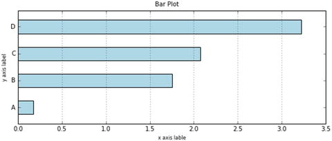
Side-by-Side Bar Chart
See Listing 2-41.
Listing 2-41. Side-by-side bar chart
# generate sample datapre = np.array([19, 6, 11, 9])post = np.array([15, 11, 9, 8])labels=['Survey '+x for x in list('ABCD')]# the plot – left then rightfig, ax = plt.subplots(figsize=(8, 3.5))width = 0.4 # bar widthxlocs = np.arange(len(pre))ax.bar(xlocs-width, pre, width,color='green', label='True')ax.bar(xlocs, post, width,color='#1f10ed', label='False')# labels, grids and title, then saveax.set_xticks(ticks=range(len(pre)))ax.set_xticklabels(labels)ax.yaxis.grid(True)ax.legend(loc='best')ax.set_ylabel('Count')fig.suptitle('Sample Chart')fig.tight_layout(pad=1)fig.savefig('filename.png', dpi=125)# ---- output ----
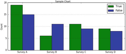
Stacked Bar Example Code
See Listing 2-42.
Listing 2-42. Stacked bar charts
# generate sample datapre = np.array([19, 6, 11, 9])post = np.array([15, 11, 9, 8])labels=['Survey '+x for x in list('ABCD')]# the plot – left then rightfig, ax = plt.subplots(figsize=(8, 3.5))width = 0.4 # bar widthxlocs = np.arange(len(pre)+2)adjlocs = xlocs[1:-1] - width/2.0ax.bar(adjlocs, pre, width,color='grey', label='True')ax.bar(adjlocs, post, width,color='cyan', label='False',bottom=pre)# labels, grids and title, then saveax.set_xticks(ticks=xlocs[1:-1])ax.set_xticklabels(labels)ax.yaxis.grid(True)ax.legend(loc='best')ax.set_ylabel('Count')fig.suptitle('Sample Chart')fig.tight_layout(pad=1)fig.savefig('filename.png', dpi=125)# ---- output ----
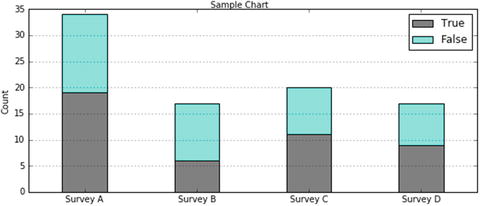
Pie Chart – Using ax.pie()
See Listing 2-43.
Listing 2-43. Pie chart
# generate sample datadata = np.array([15,8,4])labels = ['Feature Engineering', 'Model Tuning', 'Model Building']explode = (0, 0.1, 0) # explode feature engineeringcolrs=['cyan', 'tan', 'wheat']# plotfig, ax = plt.subplots(figsize=(8, 3.5))ax.pie(data, explode=explode,labels=labels, autopct='%1.1f%%',startangle=270, colors=colrs)ax.axis('equal') # keep it a circle# tidy-up and savefig.suptitle("ML Pie")fig.savefig('filename.png', dpi=125)# ---- output ----
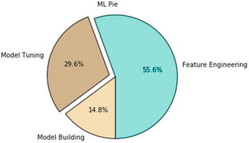
Example Code for Grid Creation
See Listing 2-44.
Listing 2-44. Grid creation
# Simple subplot grid layoutsfig = plt.figure(figsize=(8,4))fig.text(x=0.01, y=0.01, s='Figure',color='#888888', ha='left', va='bottom', fontsize=20)for i in range(4):# fig.add_subplot(nrows, ncols, num)ax = fig.add_subplot(2, 2, i+1)ax.text(x=0.01, y=0.01, s='Subplot 2 2 '+str(i+1), color='red', ha='left', va='bottom', fontsize=20)ax.set_xticks([]); ax.set_yticks([])ax.set_xticks([]); ax.set_yticks([])fig.suptitle('Subplots')fig.savefig('filename.png', dpi=125)# ---- output ----
Plotting – Defaults
Matplotlib uses matplotlibrc configuration files to customize all kinds of properties, which we call rc settings or rcparameters. You can control the defaults of almost every property in matplotlib such as figure size and dpi, line width, color and style, axes, axis and grid properties, text and font properties, and so on. The location of the configuration file can be found using the code in Listing 2-45 so that you can edit it if required.
Listing 2-45. Plotting defaults
# get configuration file locationprint (matplotlib.matplotlib_fname())# get configuration current settingsprint (matplotlib.rcParams)# Change the default settingsplt.rc('figure', figsize=(8,4), dpi=125,facecolor='white', edgecolor='white')plt.rc('axes', facecolor='#e5e5e5', grid=True, linewidth=1.0, axisbelow=True)plt.rc('grid', color='white', linestyle='-', linewidth=2.0, alpha=1.0)plt.rc('xtick', direction='out')plt.rc('ytick', direction='out')plt.rc('legend', loc='best')
Machine Learning Core Libraries
Python has a plethora of open source machine learning libraries. Table 2-4 gives a quick summary of the top 10 Python machine learning libraries ranked, based on their number of contributors, and also shows the change in percentage of growth in their contributors count between 2015 and 2016.
Table 2-4. Python machine learning libraries
Contributors | |||||
|---|---|---|---|---|---|
Project Name | 2015 | 2016 | Change (%) | License Type | Source |
Scikit-learn | 404 | 732 | 81% | BSD 3 | |
Pylearn2 | 117 | 115 | -2% | BSD 3 | |
NuPIC | 60 | 75 | 25% | AGPL 3 | |
Nilearn | 28 | 46 | 64% | BSD | |
PyBrain | 27 | 31 | 15% | BSD 3 | |
Pattern | 20 | 20 | 0% | BSD 3 | |
Fuel | 12 | 29 | 142% | MIT | |
Bob | 11 | 13 | 18% | BSD | |
Skdata | 10 | 11 | 10% | N/A | |
MILK | 9 | 9 | 0% | MIT | |
Scikit-learn is the most popular and widely used machine learning library. It is built on top of SciPy and features a rich number of supervised and unsupervised learning algorithms.
We’ll learn more about different algorithms of Scikit-learn in detail in the next chapter.
Note
StatsModels is another important library often used for running regression models; however, it does not have the implementation of other machine learning algorithms. It’s BSD-3 licensed with 110 contributors as of 2016.
Endnotes
With this we have reached the end of this chapter. We have learned what machine learning is, and where it fits in the wider artificial intelligence family. We have also learned about the different related forms/terms (such as statistics, data or business analytics, data science) that exist parallel to machine learning and why they exist. We have briefly explained the high-level categories of machine learning, and most commonly used frameworks to build efficient machine learning systems. Toward the end we learned that the machine learning libraries can be categorized into data analysis and core ML packages. We also looked at the key concepts and example implementation code for three important data analysis packages: NumPy, Pandas, and Matplotlib. I would like to leave you with some useful resources for your future reference to deepen your knowledge in the data analysis packages. See Table 2-5.
Table 2-5. Additional resources
Resource | Description | Mode |
|---|---|---|
This is a quick start tutorial for NumPy and covers all the concepts in detail. | Online | |
This is a guide to many pandas tutorials, geared mainly for new users. | Online | |
Beginners guide, Pyplot tutorial. | Online | |
Python for Data Analysis | This book is concerned with the nuts and bolts of manipulating, processing, cleaning, and crunching data in Python. | Book |