
“A real intelligence is an art to simplify complex matters without losing the integrity of that matter.”
— Sumit Singh
Our lives are complex. We have to deal with complexity everyday—at home, at work, with our commute, within family, and with our career goals. There are many paths to success, but the definition of success is subjective and complex. And we always strive to find the best ingredients to ease that path to success.
Like our lives too, data can be hugely complex at times. We need more advanced algorithms, sophisticated techniques, out-of-the-box approaches, and innovative processes to make sense of it. But the heart of any solution, any algorithm, any approach, and any process is the need to resolve the business problem at hand. Most of the business problems involve how to increase profits and to decrease costs. Using such advanced methodologies, we can make sense with the complex datasets that are generated by our systems.
In the first three chapters of the book, we studied ML for regression and classification problems using quite a few algorithms. We examined the concepts and developed Python solutions for them. In this chapter, we are going to work on advanced algorithms. We will be studying these algorithms and developing the mathematical concepts and coding logic for them. We will not be working on structured data alone. We will be working on unstructured datasets too—text and image—in this chapter.
In this chapter, advanced algorithms like boosting and SVMs will be examined. Then we will be diving into the world of text and image data, and solving such challenges using principles of natural language processing (NLP) and image analysis. Deep learning is used for solving the complex problems and hence we will be implementing deep learning to a structured data and unstructured image dataset. All the code files and datasets are provided with step-by-step explanations.
Technical Toolkit Required
We are going to use Python 3.5 or above in this book. You are advised to get Python installed on your machine. We will be using Jupyter notebook; installing Anaconda-Navigator is required for executing the codes. All the datasets and codes have been uploaded to the Github library at https://github.com/Apress/supervised-learning-w-python/tree/master/Chapter%204 for easy download and execution.
The major libraries used are numpy, pandas, matplotlib, seaborn, scikit learn, and so on. You are advised to install these libraries in your Python environment. In this chapter, we are going to use NLP so will use NLTK library and RegexpTokenizer. We will also need Keras and TensorFlow libraries in this chapter.
Let us go into the ensemble-based boosting algorithms and study the concepts in detail!
Boosting Algorithms
Recall in the last chapter we studied ensemble-modeling techniques. We discussed bagging algorithms and created solutions using random forest. We will continue with ensemble-modeling techniques. The next algorithm is boosting.
Formally put, boosting is an ensemble method that creates a strong classifier from weak classifiers. In a sequence, we create a new model while assuring we are learning from the errors or misclassifications from the previous model as shown in Figure 4-1. The idea is to give higher importance to the errors and improve the modeling subsequently, finally resulting in a very strong model.
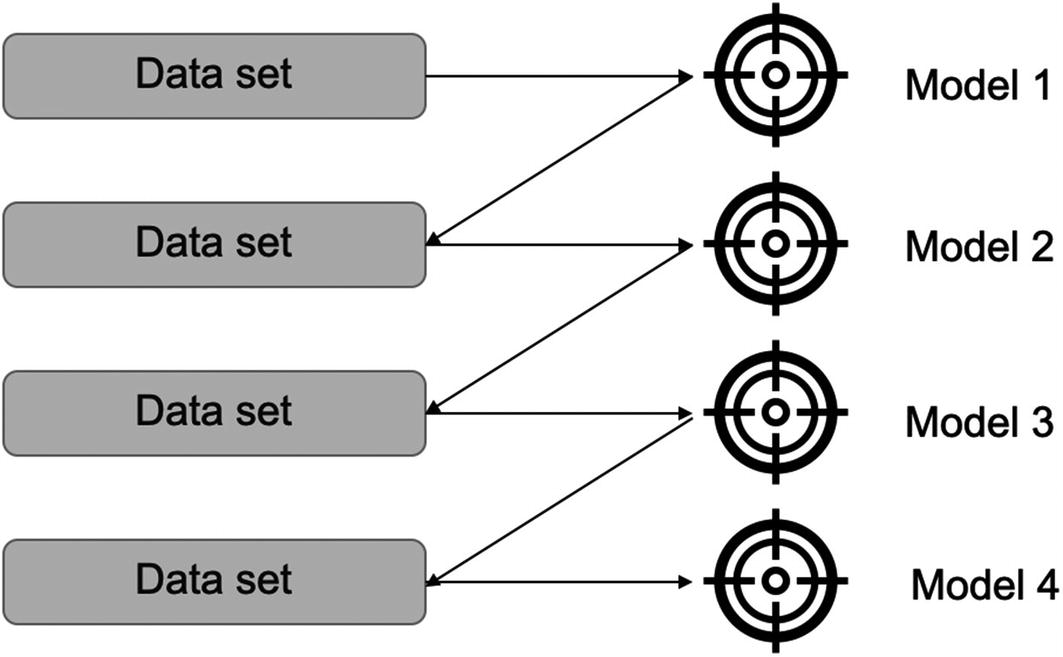
Boosting algorithms iteratively work and improve the previous version while assigning higher weights to the errors
- 1.
Gradient boosting : Gradient boosting can work for both classification and regression problems. For example, a regression tree can be used as a base learner and each subsequent tree will be an improvement over the previous tree. The overall learner gradually improves on the observations where the residuals have been initially high.
The properties of gradient boosting are as follows:- a.
A base learner is created by taking a subset of the complete dataset.
- b.
The difficult observations are identified, or the shifting is done by identifying the value of the residuals in the previous model.
- c.
The misclassifications are identified by the gradients calculated. This is the central idea of the algorithm. It creates new base learners which are correlated maximum with the negative gradient of the loss function, which in turn is associated with the complete ensemble solution.
- d.
It then further dissects error components to add more information about the residuals.
- a.
- 2.
AdaBoosting : AdaBoosting or adaptive boosting is considered as a special case of gradient boosting, wherein iterative models are created to improve upon the previous model. Initially, a base model is created using a subset of the data and is used to make predictions on the complete dataset. We measure the performance by calculating the error. Then while creating the next model, data points which have been predicted incorrectly are given higher weights. The weights are proportional to the error; that is, the higher the error, the higher is the weight assigned. Hence, the next model created is an improvement over the previous model, and this process continues. Once it is no longer possible to reduce the error further, the process stops and we conclude that we have reached the final model, which is the best model.
AdaBoost has the following properties:- a.
In AdaBoost, the shifting is done by assigning higher weights to the observations misclassified in the previous step.
- b.
The misclassifications are identified by high-weight observations.
- c.
The exponential loss in AdaBoost assigns greater value of weight for the sample which have ill-fitted in the previous model.
- a.
- 3.
Extreme gradient boosting: Extreme gradient boosting of XGB is an advanced boosting algorithm. It has become quite popular lately and has won many data science and ML competitions. It is extremely accurate and quite a fast solution to implement.
The properties for XGB are as follows:- a.
XGB is quite a fast algorithm since it allows parallel processing and hence is faster than standard gradient boosting.
- b.
It tackles overfitting by implementing regularization techniques.
- c.
It works well with messy datasets having missing values, as it has an inbuilt mechanism to handle missing values present in the dataset. This is one of the biggest advantages, as we do not have to deal with missing values present in the data.
- d.
It is quite a flexible algorithm and allows us to have a customized optimization objective and evaluation criteria.
- e.
Cross-validation at each iteration results in an optimum number of boosting iterations, which makes it a better choice than its counterparts.
- a.
- 4.CatBoost: CatBoost is a fantastic solution if we are dealing with categorical variables. In typical ML models, we use one-hot encoding to deal with categorical variables. For example, if we have a dataset having a categorical variable as “City,” we convert it to numeric variables as shown in Table 4-1.Table 4-1
One-Hot Encoding to Convert Categorical Variables to Numeric Variables
But if we have 100 unique values for the variable “City,” one-hot encoding will result in adding 100 additional dimensions to the dataset. Moreover, the resultant dataset will be quite sparse. Sparsity means that for a column only a few rows will be 1; the rest will be 0. For example, in Table 4-1 Tokyo has got only one value as 1. That means that the matrix contains more 0’s than 1’s. Hence, the performance operation across will take a long time. Moreover, if the number of resultant dimensions are too large then we will have huge memory requirements.
CatBoost does not suffer from this problem. CatBoost deals with categorical variables internally and we do not have to spend time on dealing with them.
- 5.
Light gradient boosting : As the name suggests, light gradient boosting is computationally less expensive than its counterparts. It is the choice of boosting algorithm if the dataset is extremely large. It implements tree-based algorithms and uses a leaf-based approach, as compared to others, which use a level-based approach, as shown in Figure 4-2.

Level-based approach is used by other boosting algorithms, while leaf-based approach makes light gradient boosting a good fit for large datasets
We have now discussed the different types of boosting algorithms. Depending on the business problem at hand and the data set available, we will prefer one method over another. Recently extreme gradient boosting or XGB has gained a lot of popularity. It is quite a robust technique, gives better results, and deals with overfitting internally.
We will now implement a case in Python using gradient boosting algorithm.
Using Gradient Boosting Algorithm
In this case study, we are going to implement multiple algorithms. We have studied multiple algorithms till now, and some of them are ensemble-based advanced algorithms. It is the correct time to compare their respective accuracies.
We will perform EDA, create train-test split, and then implement decision tree, random forest, bagging, AdaBoost, and gradient boosting algorithm. Finally, we will compare the respective performance of all the algorithms.
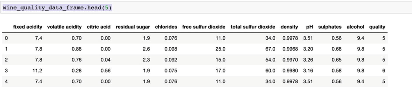
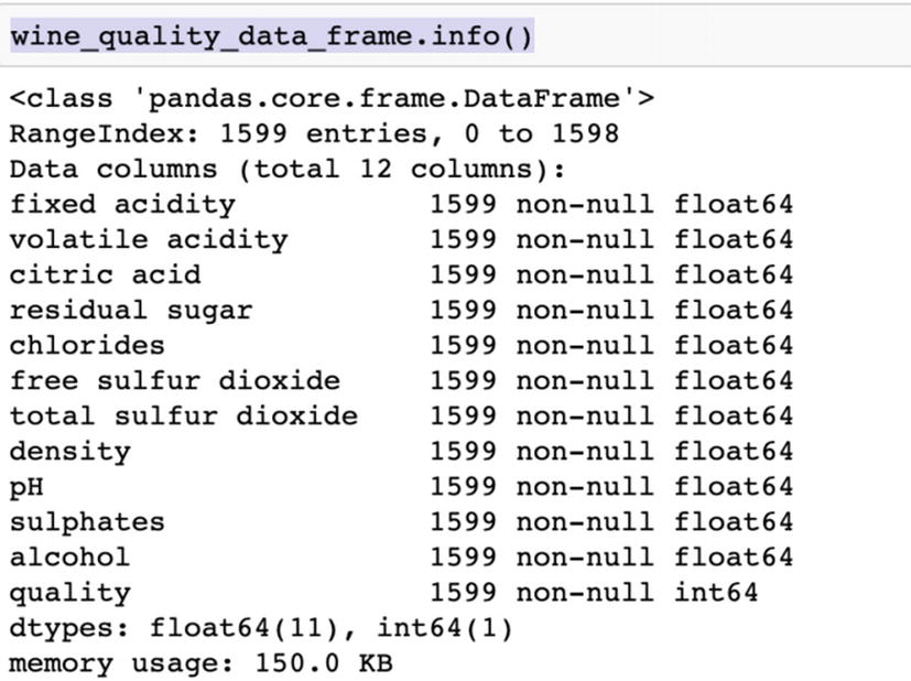
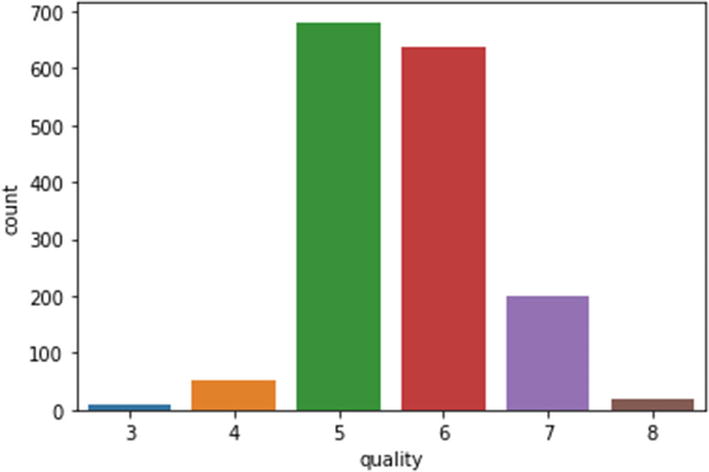
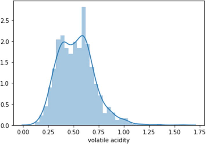
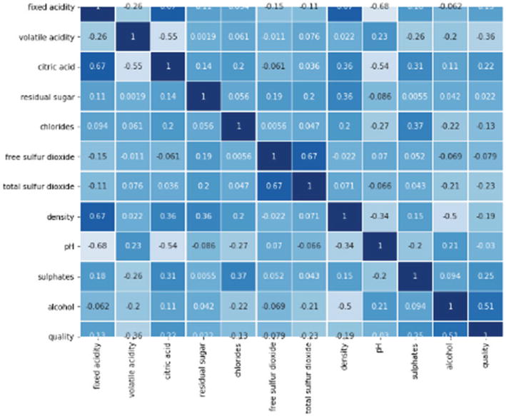
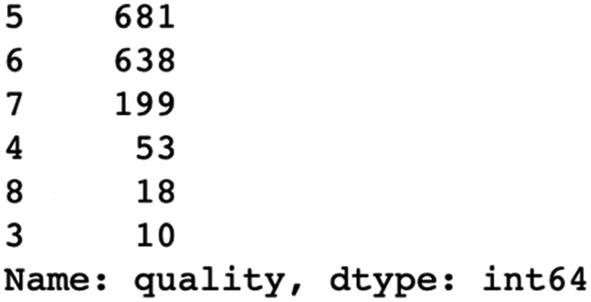
The dataset and code can be downloaded from the Github link shared at the start of the chapter. The data is for predicting wine quality based on parameters like fixed acidity, volatile acidity, and so on.

Step 11: The overfitting has been handled but accuracy has not improved.


We can deduce that random forest has given us the best accuracy as compared to the other algorithms. This solution can be extended to any supervised classification problem.
Gradient boosting is one of the most popular techniques. Its power is due to the focus it puts on errors and misclassifications. It is very useful in the field of information retrieval system where ML-based ranking is implemented. With its variants like extreme gradient boosting it can combat overfitting and missing variables and with CatBoost it overcomes the challenges with categorical variables. Along with bagging techniques, boosting is extending the predictive power of ML algorithms.
It is recommended to test random forest and gradient boosting while you are solving a real-world business problem since they offer higher flexibility and performance.
Ensemble methods are much more robust, accurate, and mature algorithms as compared to their counterparts. They enhance capabilities by combining the weak predictors and improve the overall performance. This is the reason they have outperformed other algorithms in many ML competitions. In the business world too, random forest and gradient boosting are frequently used to solve business problems.
We will now study another powerful algorithm called Support Vector Machine (SVM) , which is often used for small but complex datasets having a large number of dimensions. It is a common challenge in industries like medical research where the dataset is generally small but has a very high number of dimensions. SVM serves the purpose very well and is discussed in the next section.
SVM
We have already studied classical ML algorithms like regression, decision tree, and so on in the previous chapters. They are quite competent to solve any sort of regression or classification problems for us and work on live datasets. But for “really” complex datasets, we require much higher capability. SVMs allow us those capabilities to process those multidimensional complex data sources. Complexity of the data source will be owing to the multiple dimensions we have and due to the different types of variables present in the data. Here, SVMs help in creating a robust solution.
SVM is a fantastic solution for complex datasets, particularly where we have a dearth of training examples. Apart from the uses on structured datasets and simpler business problems, it is used for categorization of text in text analytics problems, image classification, bioinformatics field, and handwriting recognition.
SVM can be used for both regression and classification problems. The basis of SVM is on support vectors which are nothing but the representation of observations in a vector space.
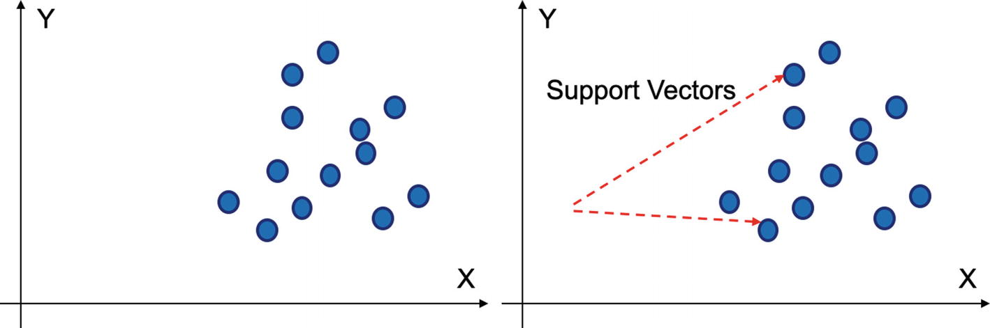
Support vectors are the representations of data points in a vector-space diagram
SVMs work on these representations or support vectors and model a supervised learning algorithm. In Figure 4-4, we have two classes which need to be differentiated. SVM fixes this problem by creating hyperplane, which is most suitable for that decision.
A hyperplane can be used to distinguish between two classes. Margin is used to select the best hyperplane
We have understood the purpose of the SVM. It is imperative we visualize them in a vector-space diagram to understand better. We are visualizing SVM in a 2-dimensional space in the next section.
SVM in 2-D Space
In a 2-dimensional space, the separating hyperplane is a straight line. And the classification is achieved by a perceptron.
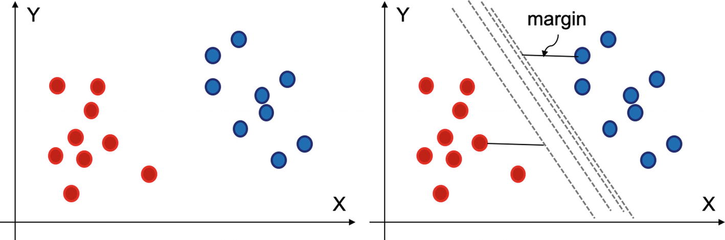
A perceptron is an algorithm used to make binary classification. Simply put, it is trained on data with two classes and then it outputs a line that separates two classes clearly. In Figure 4-5, we can try to achieve a hyperplane or a line which segregates the two classes.
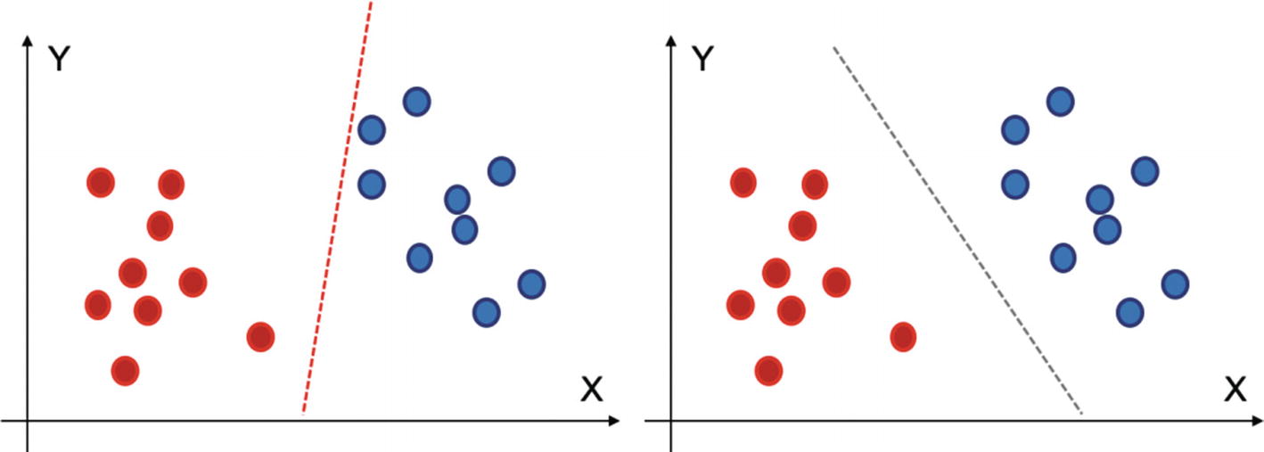
The red line, though able to classify between two classes, suffers from high variance. The black classifier on the right is better than the red one
So, we have decided that the second line is better than the first line. Let us say that the equation of the line is ax + by = c. Hence, the equation for the classification plane can be ax + by ≥ c for the red dots and ax + by < c for the blue ones.
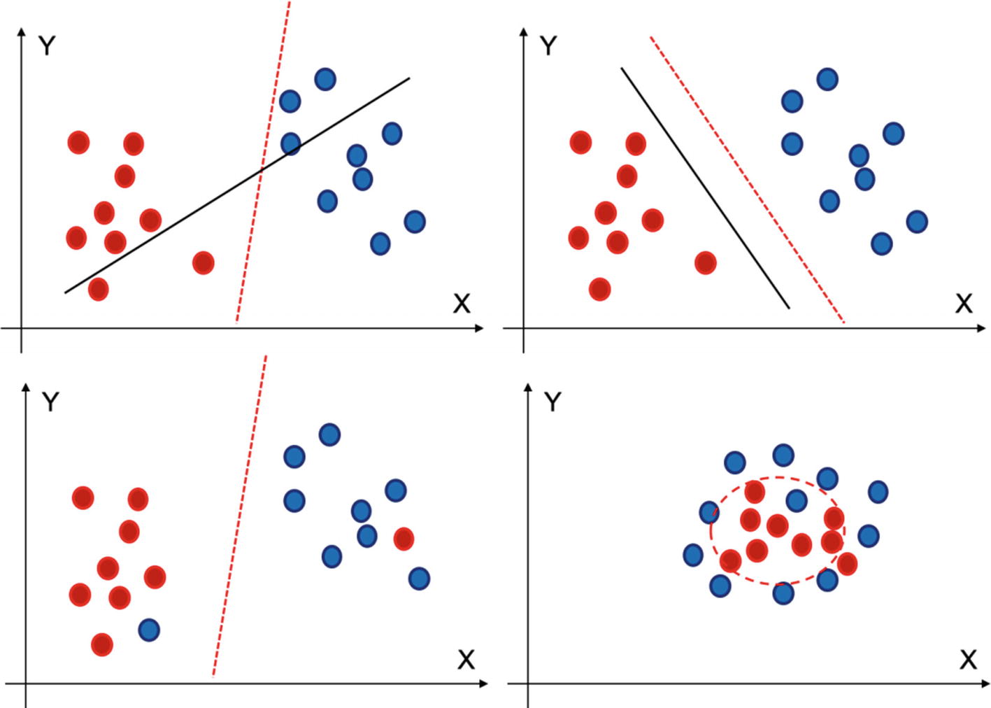
But there can be a lot of options for a, b, or c, which brings us to the next question: how to choose the best plane. As shown in Figure 4-6, there can be a number of options available for the hyperplanes.
In Figure 4-6, for the figure on top left, the red separator is doing a better job in classifying the two classes than the black solid line. In the second figure, we can see that the red separator has a maximum margin as compared to the black one, hence it is chosen.

(i) At top left, the red classifier is better than the black one. (ii) In the second one, red is better as it has maximum margin. (iii) The third one has outliers but still SVM will be able to handle it. (iv) This is a special case where linear classifier will not be able to distinguish between the two classes
So far, we have discussed and visualized the implementations in a 2-D space, but if were to transform the mathematical vector space from a 2-dimensional one to higher dimensions, then we need to perform such mathematical operations. In Figure 4-6, the fourth figure is such a special case. In the case shown, it is not possible to have a linear hyperplane, and in such a case we will have a nonlinear hyperplane to make the classifications for us, which is possible using kernel SVM (KSVM) , which we are discussing next.
KSVM
The fourth diagram is implementing a nonlinear classifier to distinguish between two classes
KSVM has created a nonlinear classifier to perform the classification between the two classes.
- 1.
Kernel: Kernel is used when we have the data which can become separable if expressed in higher dimensions. The various kernels available in sklearn are rbf, poly, sigmoid, linear, precomputed, and so on. If we use a “linear” kernel, it will use a linear hyperplane or a line in the case of 2-dimensional data. ‘rbf’, ‘poly’ are used for nonlinear hyperplanes .
- 2.
C: C is used to represent the misclassification error or the cost parameter. If the value of C is low, the penalty of misclassification observations is low and hence the accuracy will be high. It is used to control the tradeoff between accurate classification of training data and having a smooth decision boundary.
- 3.
Gamma: Gamma is used to define the radius of influence of the observations in a classification. It is primarily used for nonlinear hyperplanes. A higher gamma can lead to better accuracy, but results can be biased, and vice versa.
We have to iterate with various values of such parameters and reach the best solution. With a high value of gamma, the variance will be low and bias will be high, and vice versa. And when the value of C is large, variance will be high and bias will be low, and vice versa.
There are both advantages and some challenges with using SVM.
- 1.
It is a very effective solution for complex datasets, where the number of dimensions is large .
- 2.
It is the preferred choice when we have more dimensions and less training dataset.
- 3.
The margin of separation by SVM is quite clear and provides a good, accurate, and robust solution.
- 4.
SVM is easy to implement and is quite a memory-efficient solution to implement.
- 1.
It takes time to converge with large sample size and hence may not be preferred for bigger datasets.
- 2.
The algorithm is sensitive to messy data. If the target classes are not clearly demarcated and different, the algorithm tends to perform not so well.
- 3.
SVM does not provide direct probabilities for the predictions. Instead they have to be calculated separately.
Despite a few challenges, SVM has repeatedly proven its worth. It offers a robust solution when we have a multidimensional smaller data set to analyze. We are now going to solve a case study in Python using SVM now.
Case Study Using SVM
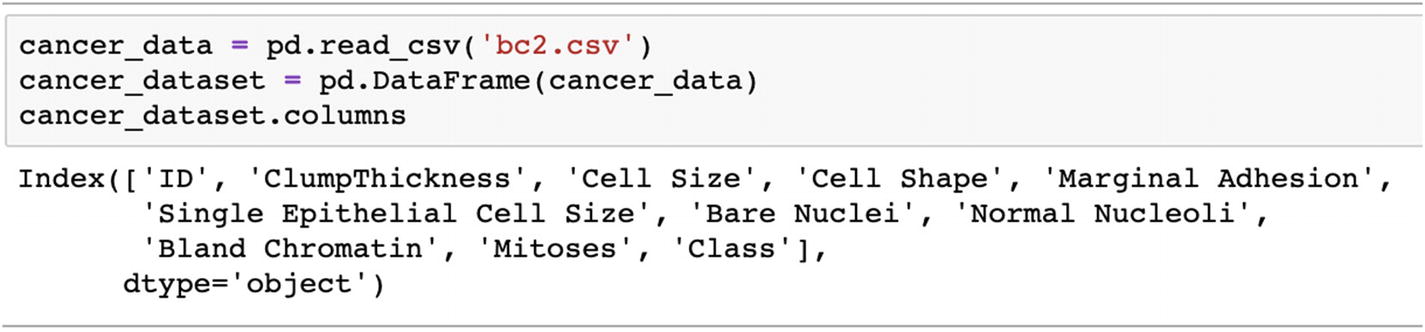
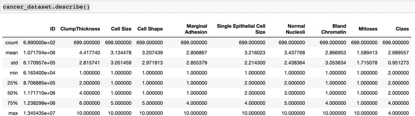
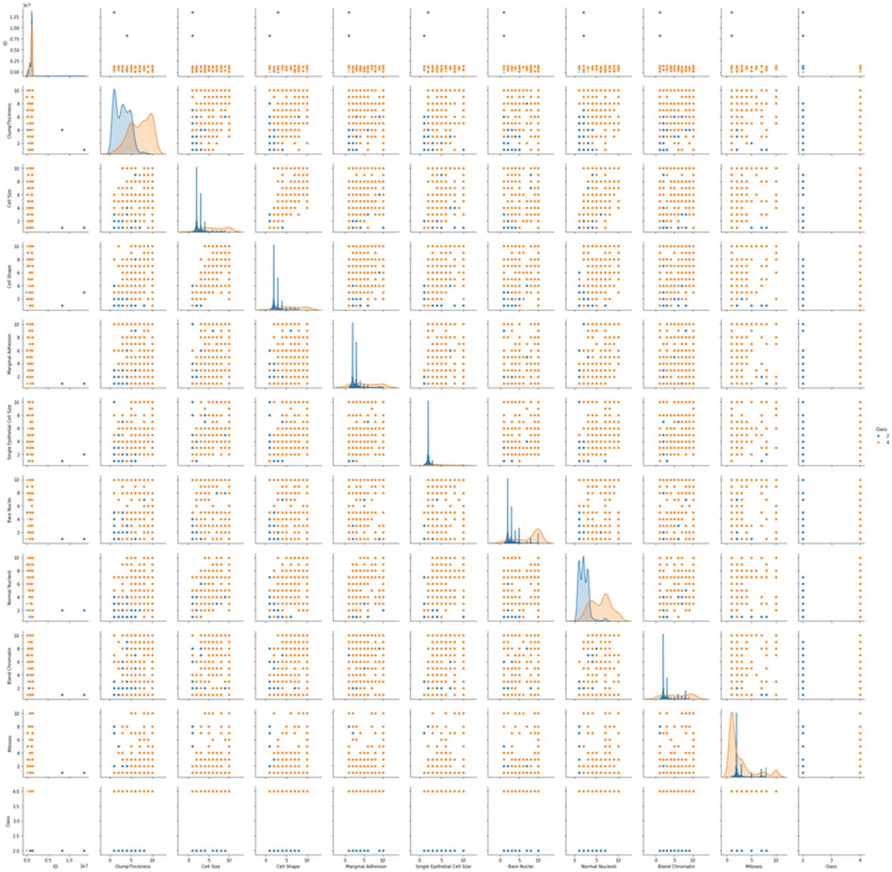
We are solving a cancer detection case study. The dataset is available at the Github link shared at the start of the chapter.


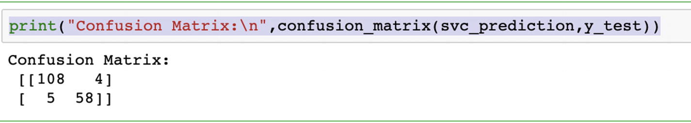
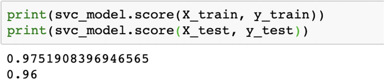

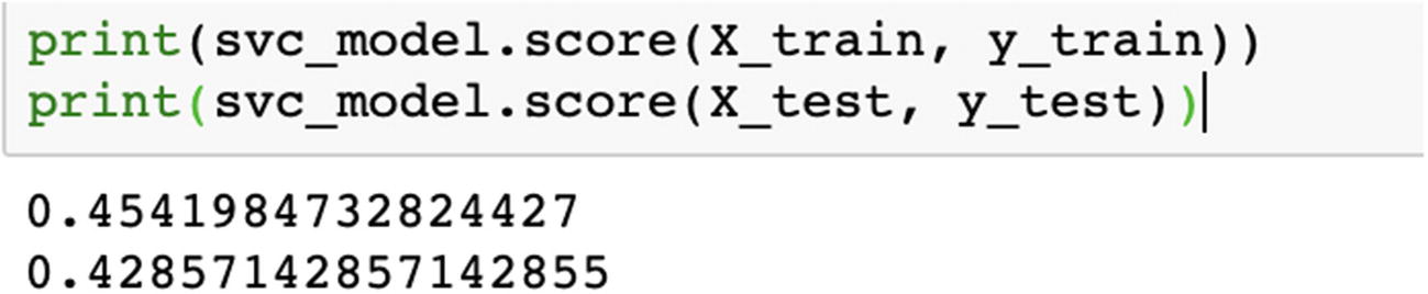
We can compare the respective accuracies for all the kernels and choose the best one. Ideally, accuracy should not be the only parameter; we should also compare recall and precision using confusion matrix.
In the preceding example, we created a Python solution using SVM. When we change the kernel, the accuracy changes a lot. The SVM algorithm should be compared along with other ML models and then the best algorithm should be chosen.
Ideally we test any problem with three or four algorithms and compare the precision, recall, accuracy and then decide which algorithm is best for us. These steps are discussed again in Chapter 5.
With this we have studied the SVM in detail. An easy-to-implement solution, SVM is one of the advanced supervised learning algorithms which is heavily recommended.
So far, we have studied and created solutions for structured data. We started with regression, decision trees, and so on in previous chapters. We examined the concepts and created a solution in Python. In this chapter, we continued with boosting algorithms and SVMs. Now we will start a much more advanced topic—supervised learning algorithms for unstructured data, which are text and images, in the next section. We will study the nuts and bolts, preprocessing steps, challenges faced, and use cases. And like always, we will create Python solutions to complement the knowledge.
Supervised Algorithms for Unstructured Data
We now have access to cameras, phone, processors, recorders, data management platforms, cloud-based infrastructure, and so on. And hence, our capabilities to record data, manage it, store it, transform it, and analyze it have also improved tremendously. We are not only able to capture complex datasets but also store them and process them. With the advent of neural network–powered deep learning, the processing has improved drastically. Deep learning is a revolution in itself. Neural networks are fueling the limitless capabilities being developed across domains and business. With superior processing powers, and more powerful machines like multicore GPU and TPU, sophisticated deep neural networks are able to process more information much faster, which is true for both structured and unstructured datasets. In this section, we are going to work on unstructured datasets and study supervised learning algorithms for unstructured datasets.
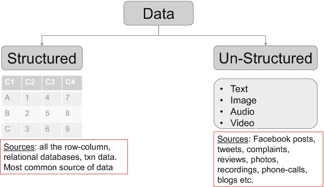
Data can be classified between structured and unstructured datasets
We will start studying the text data. We will examine all the concepts of cleaning the text data, preprocessing it, creating supervised learning solutions in Python using it, and what are the best practices to work with it. Let’s kick off now!
Text Data
Language is a gift to humanity. It is the most common medium to express ourselves. Language is involved in most interactions we have like speaking, messaging, writing, listening. This text data is everywhere. We generate it every day in the form of news, Facebook comments and posts, customer reviews and complaints, tweets, blogs, articles, literature, and so on. The datasets generated represent a wide range of emotions and expressions which are generally not captured in surveys and ratings. We do witness that in the form of online product reviews given by customers. The number of ratings given can be 5 out of 5, but the actual review text might give a different impression. Thus, it becomes even more crucial for businesses worldwide to pay attention to the text data.
Text data is much more expressive and direct. This data is to be analyzed as it holds the key to a lot of understanding we can generate about our customers, processes, products and services, our culture, our world, and our thoughts. Moreover, with the advent of Alexa, Google Assistant, Apple Siri, and Cortana the voice command is acting as an interface between humans and machines and generating more datasets for us. Massive and expressive, right!
Similar to the complexity, text data is a rich source of information and actions. Text data can be used for a plethora of solutions, which we discuss next.
Use Cases of Text Data
Text data is very useful. It expresses what we really feel in words. It is a powerful source to gauge the thoughts which often are not captured in surveys and questionnaires. It is directly sourced data and hence is less biased, though it can be a really noisy dataset to deal with.
- 1.
News categorization or document categorization : We can have incoming news or a document. We want to categorize whether a news item belongs to sports, politics, science, business, or any other category. Incoming news will be classified based on the content of the news, which is the actual text. News about business will be different from a news article on sports as shown in Figure 4-9. Similarly, we might want to categorize some medical documents into their respective categories based on the domain of study. For such purposes, supervised learning classification algorithms can be used to solve the problems.
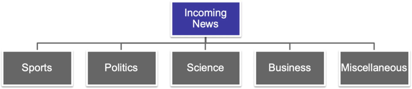
There can be multiple categories of incoming news as sports, politics, science, business, and so on
- 2.Sentiment analysis : Sentiment analysis is gauging what is the positiveness or negativity in the text data. There can be two such use cases:
- a.
We receive reviews from our customers about the products and services. These reviews have to be analyzed. Let’s consider a case. An electric company receives complaints from its customers, reviews about the supply, and comments about the overall experience. The streams can be onboarding experience, ease of registration, payment process, supply reviews, power reviews, and so on. We want to determine the general context of the review—whether it is positive, negative, or neutral. Based on these comments, an improvement can be made on the product features or service levels.
- b.
We might also want to assign a review to a specific department. For example, in the preceding case an incoming review will have to be shared with the relevant department. Using Natural Language Processing (NLP), this task can be done, the review can be shared with the finance department or operations team, and the respective team can follow up with the review and take the next course of action .
- a.
- 3.
Language translation : Using NLP and deep learning, we are able to translate between languages (e.g., between English and French). A deep neural network requires training on the vocabulary and grammar of both the languages and multiple other training data points.
- 4.
Spam filtering : Email spam filter can be composed using NLP and supervised ML. We can train an algorithm which can analyze incoming mail parameters and give a prediction if that email belongs to a spam folder or not. Going even one step further, based on the various parameters like sender email-id, subject line, body of the mail, attachments, time of mail, and so on, we can even determine if that is a promotional email or spam or an important one. Supervised learning algorithms help us in making that decision and automating the entire process.
- 5.
Text summarization of the entire book or article can be done using NLP and deep learning. In this case too, we will be using deep learning and NLP to generate summaries of entire documents or articles. This helps in creating us an abridged version of the text.
- 6.
Part-of-speech (POS) tagging : POS tagging refers to the identification of words as nouns, pronouns, adjectives, adverbs, conjunctions, and so on. It is the process of marking the words in the text corpus corresponding to a particular POS, based on its use, definition, and context in the sentence and larger body, as shown in Figure 4-10.
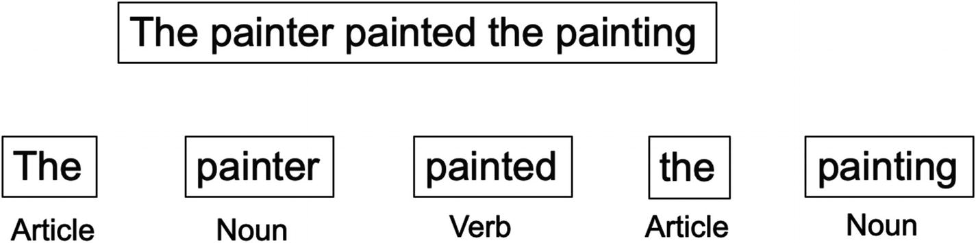
POS tagging for words into their respective categories
Text data can be analyzed using both supervised and unsupervised problems. We are focusing on supervised learning in this book. We use NLP to solve the problems. And deep learning further improves the capabilities we have. These are the tools which empower us to deal with such complex datasets.
But text data is difficult to analyze. It has to be still represented in the form of numbers and integers; only then can it be analyzed. Our computers and processors understand numbers and the algorithms also expect numbers only. We will now discuss the most common challenges we face with text data in the next section.
Challenges with Text Data
Text is perhaps the most difficult data to be analyzed and worked with. The number of permutations to express the same question or thought are many. For example, “what is your age” and “how old are you” mean one and the same thing. We have to resolve these challenges and come up with a dataset which is robust, complete, and representative while at the same time not losing the original context.
- 1.
Language is unbounded. It changes every day and every moment new words are added to the dictionaries.
- 2.
Languages are many: Hindi, English, French, Spanish, German, Italian, and so on. Each language follows its own rules and grammar, which are unique in usage and pattern. Some are written left to right; some might be right to left or maybe even vertically! A thought which is expressed in twelve words in one language might be expressed in only five words in another.
- 3.
A word can change its meaning in a different context. For example, “I want to read this book” and “Please book the hotel for me.” A word can be an adjective and can be a noun too depending on the context.
- 4.
A language can have many synonyms for the same word; for example, “good” can be replaced by “positive,” “wonderful,” “superb,” and “exceptional” in different scenarios. Similarly, words like “study,” “studying,” and “studies” are related to the same root word, “study.”
- 5.
Words can completely even change their meaning with usage. For example, “apple” is a fruit, while “Apple” is a company producing Macintosh. “Tom” can be a name but when used as “Tom Software Consulting,” its usage is completely changed.
- 6.
Tasks which are very easy for humans might be very difficult for machines. We do have memory, while machines tend to forget. For example, “John is from London and he moved to Australia and is working with Allan over there. He missed his family back there.” Humans can easily recall and understand that “he” in the second sentence is John and not Allan.
These are not the only challenges, and the preceding list is not exhaustive. Managing this massive dataset, storing it, cleaning it, and refreshing it is a Herculean task in itself. But using sophisticated processes and solutions, we are able to resolve most of them, if not all. Some of these techniques we discuss in the next section on preprocessing the text data and extracting the features from the text data.
Like any other ML project, text analytics follow the principles of ML, albeit the process is slightly different. We will discuss the text analytics process now in the next section.
Text Analytics Modeling Process
Text analytics is complex owing to the complexity of data we are dealing with and the data preprocessing required. At a high level the various process heads remain the same, but still a lot of the subprocesses are customized for text. They are also dependent on the business problem we want to solve. The typical text analytics process is shown in Figure 4-11.

End-to-end process in a text analytics project from data collection to the deployment
- 1.
Our customer’s satisfaction regarding the products and services.
- 2.
The major pain points and dissatisfactions, what drives the engagement, which services are complex and time-consuming, and which are the most liked services.
- 3.
The products and services which are most popular, which are least popular, and any popularity patterns.
- 4.
How best to represent these findings by means of a dashboard. This dashboard will be refreshed at a regular cycle like monthly or quarterly refresh.
- 1.
The products and services which are most satisfactory and are most liked ones should be continued.
- 2.
The ones which are receiving a negative score have to be improved and challenges have to be mitigated.
- 3.
The respective teams like finance, operations, complaints, CRM, and so on can be notified, and they can work individually to improve the customer experience.
- 4.
The precise reasons for liking or disliking the services will be useful for the relevant teams to work in the correct direction.
- 5.
Overall, it will provide a benchmark to measure the Net Promoter Score (NPS) for the customer base. The business can strive to enhance the overall customer experience.
A concise, precise, measurable, and achievable business problem is the key to success. Once the business problem is frozen, we will work on securing the dataset, which we will discuss next.
Text Data Extraction and Management
As discussed in the last section, customer text data can be generated through a number of sources. The entire dataset in text analytics is referred to as a corpus. Formally put, a corpus represents a large collection of text data (generally labeled but can be unlabeled too), which is used for statistical analysis and hypothesis testing.
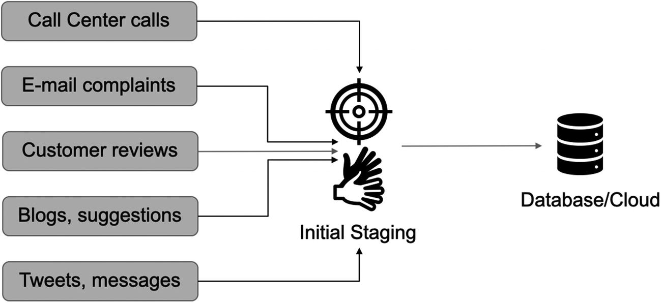
Data management process of text data, starting from data collection to the final storage
Customer Reviews Having Customer Details Like ID, Date, Product, City, and Actual Review Text
|
Here, we have the unique customer ID, product purchased, date of the review, city, source, and actual review text of the customer. This table can have many more data points then we have shown. And there can be other tables having customer details like was the complaint resolved, time to resolve, and so on, which can serve as additional information to analyze.
All such data points have to be maintained and refreshed. The refresh cycle can be determined as per the business requirements: it can be a monthly, quarterly, or yearly refresh.
There is one more important source of data which is very insightful and can be used for wider strategy creation. There are plenty of online channels and platforms where a customer can review a product/service. Online marketplaces like Amazon also have details of customer reviews. These platforms have reviews of the competitive brands too. For example, Nike might be interested in Puma’s and Reebok’s customer reviews. These online reviews have to be scraped and maintained. Again, these reviews might be in a different format and will have to be cleaned.
During this data maintenance phase, we clean a lot of text data like junk characters like *&^# which are present in the data. They might occur because of formatting errors while loading the data or the data itself might have junk characters. The text data is cleaned to the maximum possible extent, and further cleaning can take place in the next step of data preprocessing.
Text data is really tough data to deal with. There are a lot of complexities and data is generally messy. We have discussed a few of the challenges in the last section. We will be examining a few again and examining solutions to tackle them in the next section. We are starting with extracting features from the text data, representing them in a vector-space diagram and creating ML models using these features.
Preprocessing of Text Data
Text data, like any other data source, can be messy and noisy. We clean some of it in the data discovery phase and a lot of it in the preprocessing phase. At the same time, we have to extract the features from our dataset. This cleaning process is a standard one and can be implemented on most of the text datasets.
There are multiple processes in which we complete these steps. We will start with cleaning the raw text first.
Data Cleaning
There is no second thought about the importance of data quality. The cleaner the text data is, the better the analysis will be. At the same time, reducing the size of the text data will result in a lower-dimensional data. And hence, the processing during the ML phase and training the algorithms become less complex and time-consuming.
- 1.
Stop-word removal : Stop words are the most common words in a vocabulary which carry less importance than the keywords. For example, “is,” “an,” “the,” “a,” “be,” “has,” “had,” “it,” and so on. It reduces the dimensions of the data and hence complexity is reduced. But due caution is required while we remove stop words. For example, if we ask the question “Is it raining?” then the answer “It is” is a complete answer in itself.
When we are working with problems where contextual information is important like machine translation, we should avoid removing stop words.
- 2.
Library-based cleaning : This involves cleaning of data based on a predefined library. We can create a repository of words which we do not want in our text and can iteratively remove from the text data. This approach is preferred if we do not want to use a stop-word approach but want to follow a customized one.
- 3.
Junk characters : We can remove URL, hashtags, numbers, punctuations, social media mentions, special characters, and so on from the text. We have to be careful as some words which are not important for one domain might be quite useful for a different domain.
Due precaution is required when data is cleaned. We have to always keep the business context in mind while we remove words or reduce the size.
- 4.
Lexicon normalization : Depending on the context and usage, the same word might get represented in different manners. During lexicon normalization we clean such ambiguities. The basic idea is to reduce the word to its root form. Hence, words which are derived from each other can be mapped to the central word provided they have the same core meaning.
For example, study might get represented as study, studies, studied, studying, and so on as shown in Figure 4-13. The root word “study” remains the same, but its representations differ.
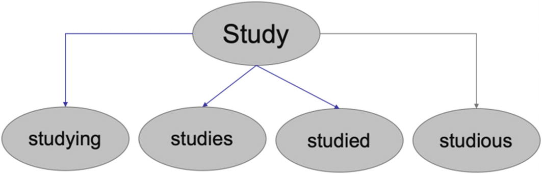
The root word is “study,” but there are many forms of it like “studying” and “studies”
There are two ways to deal with this, namely, stemming and lemmatization:
- a.
Stemming is a very basic rule-based approach of removing “es,” “ing,” “ly,” “ed,” and so on from the end of the word. For example, “studies” will become “studi” and “studying” will become “study.” As visible being a rule-based approach, the output spellings might not always be accurate.
- b.
In contrast to stemming, lemmatization is an organized approach which reduces words to their dictionary form. A lemma of a word is its dictionary or canonical form. For example, “studies,” “studied,” and “studying” all have the same root word, “study.”
- 5.
Standardization: With the advent of modern communication devices and social media, our modes of communications have changed. Along with it, our language has also changed. We have new limitations and rules, like a tweet can be of 280 characters only.
Hence, the dictionaries have to change too. We have newer references which are not a part of any standard dictionary, are ever-changing, and are different for each language, country, and culture. For example, “u” refers to “you,” “luv” is “love,” and so on.
We have to clean such text too. In such a case, we create a dictionary of such words and replace them with the correct full form.
These are only some of the methods to clean the text data. These techniques should resolve most of the issues. Still, we will not get completely clean data. Business acumen is required to further make sense to it.
Once the data is cleaned, we have to start representation of data so that it can be processed by ML algorithms—our next topic.
Extracting Features from Text Data
Text data, like any other data source, can be messy and noisy. We clean some of it in the data discovery phase and in the preprocessing phase. Now the data is clean and ready to be used. The next step is to represent this data in a format which can be understood by our algorithms.
In the simplest understanding, we can simply perform one-hot encoding on our words and represent them in a matrix. The words can be first converted to lowercase and then sorted in an alphabetical order. And then a numeric label can be assigned. And finally, words are converted to binary vectors. We will explain it using an example.
- 1.
We will convert the words to lowercase, resulting in – he, is, going, outside.
- 2.
Next, arrange the words in alphabetical order, which gives the output as – going, he, is, outside.
- 3.
We can now assign values to each word as going:0, he:1, is:2, outside:3.
- 4.
Finally, they are transformed to binary vectors as
[[0. 1. 0. 0.] #he
[0. 0. 1. 0.] #is
[1. 0. 0. 0.] #going
[0. 0. 0. 1.]] #outside
Though this approach is quite intuitive and simple to comprehend, it is pragmatically not possible due to the massive size of the corpus and the vocabulary. Moreover, handling such data size with so many dimensions will be computationally very expensive. The resulting matrix thus created will be very sparse too. Hence, we look at other means and ways to represent our text data.
There are better alternatives available to one-hot encoding. These techniques focus on the frequency of the word or the context in which the word is being used. This scientific method of text representation is much more accurate, robust, and explanatory. It generates better results too.
There are multiple such techniques like tf-idf, bag-of-words (BOW) approach, and so on. We discuss a few of these techniques in the next sections. But we will examine the important concept of tokenization first!
Tokenization
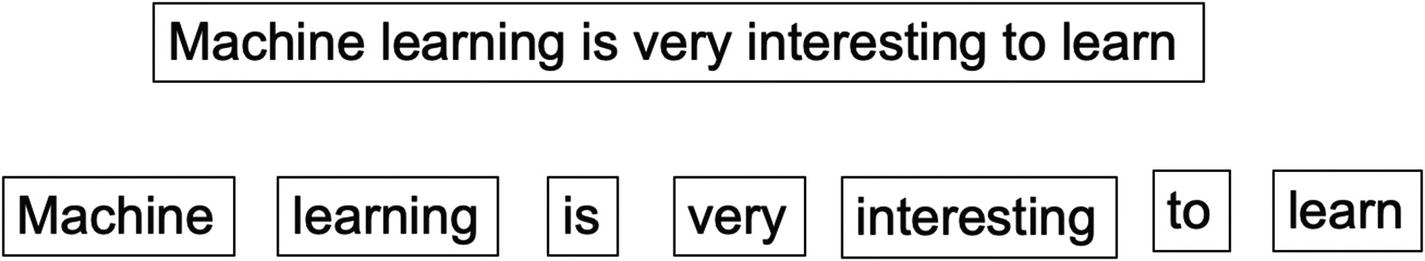
Tokenization of a sentence results in individual tokens for all the words
In the case of subwords, the same sentence can have subword tokens as interest-ing. For tokenization at a character level, it can be i-n-t-e-r-e-s-t-i-n-g. In fact, in the one-hot encoding approach discussed in the last section as a first step, tokenization was done on the words.
There are multiple methods of tokenizing based on the regular expressions to match either tokens or separators between tokens. Regexp tokenization uses the given pattern arguments to match the tokens or separators between the tokens. Whitespace tokenization treats any sequence of whitespace characters as a separator. Then we have blankline which uses a sequence of blank lines as a separator. And wordpunct tokenizes by matching sequence of alphabetic characters and sequence of non-alphabetic and non-whitespace characters.
Tokenization hence allows us to assign unique identifiers or tokens to each of the words. These tokens are further useful in the next stage of the analysis.
Now, we will explore more methods to represent text data. The first such method is the “bag of words.”
Bag-of-Words Model
In the bag-of-words approach , or BOW, text is tokenized for each observation it finds and then the respective frequency of each token is calculated. This is done disregarding grammar or word order; the primary goal is to maintain simplicity. Hence, we will represent each text (sentence or a document) as a bag of its own words.
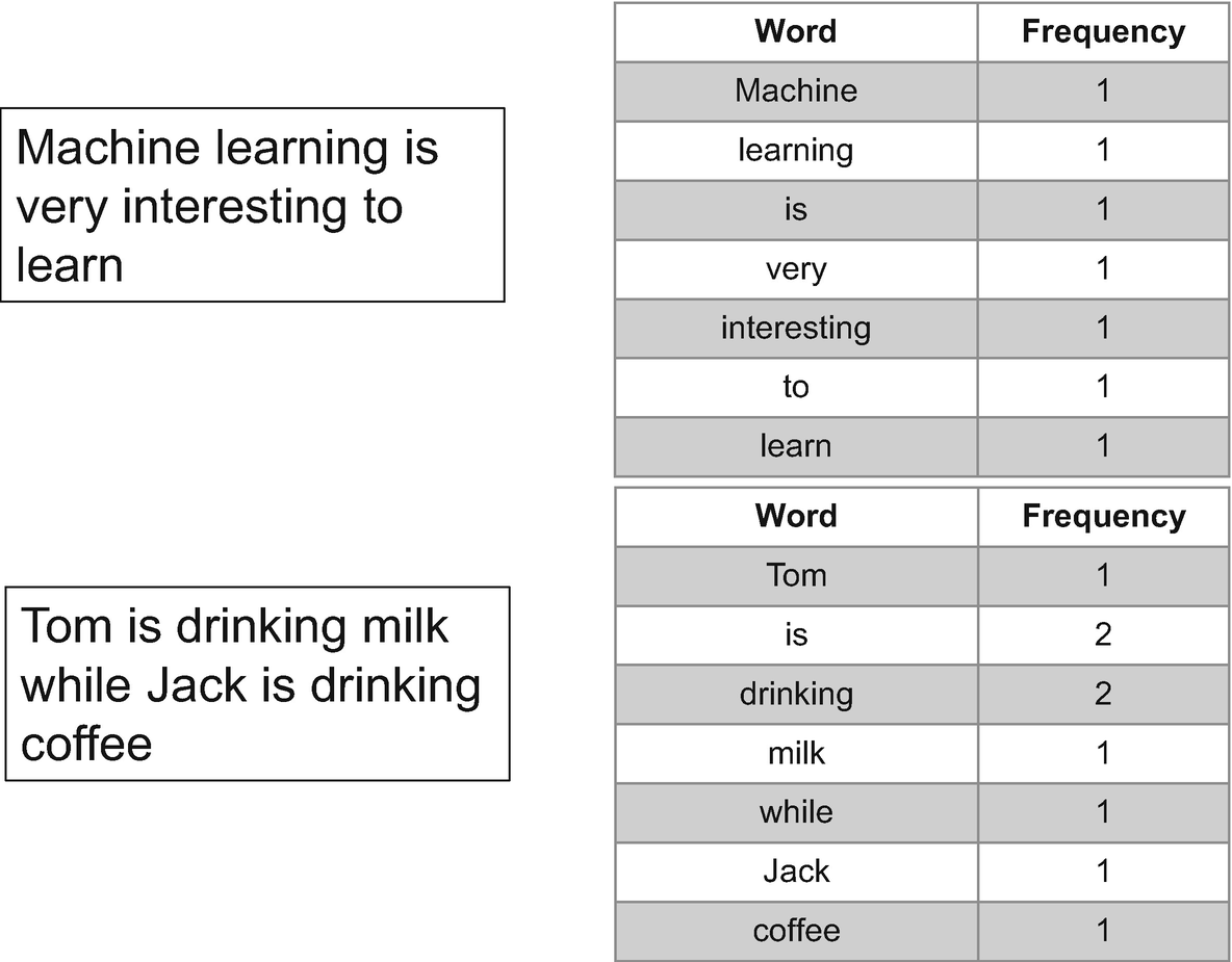
Bag-of-words approach showing that words with higher frequency are given higher values
In the BOW approach for the entire document, we define the vocabulary of the corpus as all the unique words present in the corpus. We can also set a threshold, that is, the upper and lower limit for the frequency. Then each sentence or document is defined by a vector of the same dimension as the base vocabulary containing the frequency of each word of the vocabulary in the sentence.
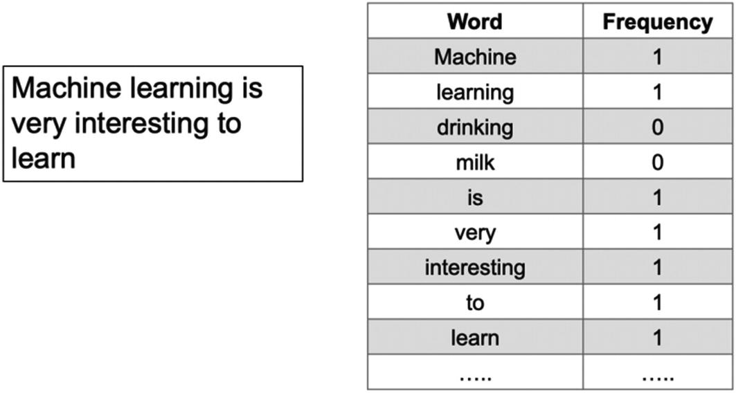
Bag-of-words representation of a sentence based on the entire vocabulary
The BOW approach has not considered the order of the words or the context. It focuses only on the frequency of the word. Hence, it is a very fast approach to represent the data. Since it is frequency based, it is commonly used for document classifications. At the same time, owing to pure frequency-based methods the model accuracy can take a hit. And that is why we have other advanced methods which consider more parameters then frequency alone. One of such methods is tf-idf or term frequency and inverse-document frequency, which we are studying next .
Term-Frequency and Inverse-Document Frequency
In the bag-of-words approach, we gave importance to the frequency of a word only. In term-frequency and inverse-document-frequency (tf-idf), we consider the relative importance of the word. tf-idf is made up of tf (term frequency) and idf (inverse-document frequency).
Term frequency (tf) is the count of a term in the entire document. For example, the count of the word “x” in the document “d.”
Inverse-document frequency (idf) is the log of the ratio of total documents (N) in the entire corpus and number of documents (df) which contain the word “x.”
So, the tf-idf formula will give us the relative importance of a word in the entire corpus. It is a multiplication of tf and idf and is given by
wi, j = tfi, j × log (N/dfi) (Equation 4-1)
where N is the total number of documents in the corpus
tfi,j is the frequency of the word in the document
dfi is the number of documents in the corpus which contain that word.
Let’s understand this with an example.
Consider we have a collection of 1 million medical documents. In these documents, we want to calculate tf-idf value for the words “medicine” and “penicillin.”
Let’s assume that there is a document of 100 words having “medicine” five times and “penicillin” only twice. So tf for “medicine” is 5/100 = 0.05 and for “penicillin” is 2/100 = 0.02.
Now, we assume that “medicine” appears in 100,000 documents out of 1 million documents, while “penicillin” appears only in 10. So, idf for “medicine” is log (1,000,000/100,000) = log (10) = 1. For “penicillin” it will be log (1,000,000/10) = log (100,000) = 5.
Hence, the final values for “medicine” and “penicillin” will be 0.05×1 = 0.05 and 0.02×5 = 0.1, respectively.
In the preceding example, we can clearly deduce that using tf-idf the relative importance of “penicillin” for that document has been identified. This is the precise advantage of tf-idf; it reduces the impact of tokens that occur quite frequently. Such tokens which have higher frequency might not offer any information as compared to words which are rare but carry more importance and weight.
The next type of representations we want to discuss are n-grams and language models.
N-gram and Language Models
In the last sections we have studied the bag-of-words approach and tf-idf. Now we are focusing on language models. We understand that to analyze the text data they have to be converted to feature vectors. N-gram models help in creating those feature vectors so that text can be represented in a format which can be analyzed further.
Language models assign probabilities to the sequence of words. N-grams are the simplest in language models. In the n-gram model we calculate the probability of the Nth word given the sequence of (N–1) words. This is done by calculating the relative frequency of the sequence occurring in the text corpus. If the items are words, n-grams may be referred to as shingles. Hence, if we have a unigram it is a sequence of one word, for two words it is bi-gram, for three words it is tri-gram, and so on. Let us study by means of an example.
Consider we have a sentence, “Machine learning is very interesting.” This sentence can be represented using N=1, N=2, and N=3. You should note how the sequence of words and their respective combinations are getting changed for different values of N, as shown in Figure 4-17.
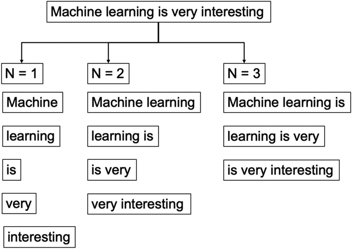
Unigram, bi-gram, tri-gram representation of the same sentence showing different results
Generally, N > 1 is considered to be much more informative than unigrams. But this approach is very sensitive to the choice of N. It also depends significantly on the training corpus which has been used, which makes the probabilities heavily dependent on the training corpus. So, if we have trained an ML model using a known corpus, we might face difficulties when we encounter an unknown word.
We have studied concepts to clean the text data, tokenize the data, and represent it using multiple techniques. It is time for us to create the first solution in NLP using Python.
Case study: Customer complaints analysis using NLP
In the last section, we examined how to represent text data into feature spaces which can be consumed by an ML model. It is the only difference a text data has from a standard ML model we have created in previous chapters.
In other words, the preprocessing and feature extraction will clean the text data and generate features. The resultant features can then be consumed by any standard supervised learning problem. After the step of feature extraction, a standard ML approach can be followed. We will now solve a case on text data and will create a Python supervised learning algorithm.
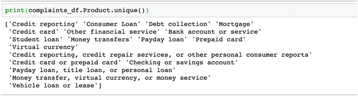
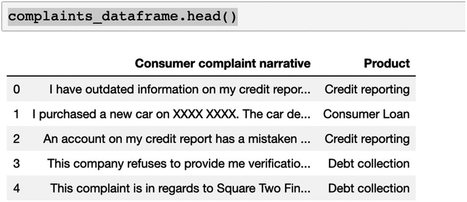
Consider we have a dataset of customer complaints. For each customer complaint, we have a corresponding product related to it. We will be using NLP and ML to create a supervised learning model to assign any incoming new complaint to the corresponding product.
The dataset and the code have been uploaded to the Github link shared at the start of the chapter.

The accuracy of the model is 76.56%. This standard model can be applied to any supervised classification problem in text analytics. Here we have a multiclass model. It can be scaled down to a binary classification as (Pass/Fail) or to create a sentiment analysis model like (positive, neutral, negative).
We have studied bag-of-words, tf-idf, and N-gram approaches so far. But in all of these techniques, the relationship between words has been neglected. We will now study an important concept which extends the learnings we have in the light of relationships between words—and it is called word embeddings .
Word Embeddings
In the last sections, all the techniques discussed ignore the contextual relationship between words. At the same time, the resultant data is very high-dimensional. Word embeddings provide a solution to the problem. They convert the high-dimensional word features into lower dimensions while maintaining the contextual relationship. We can understand the meaning by looking at an example.
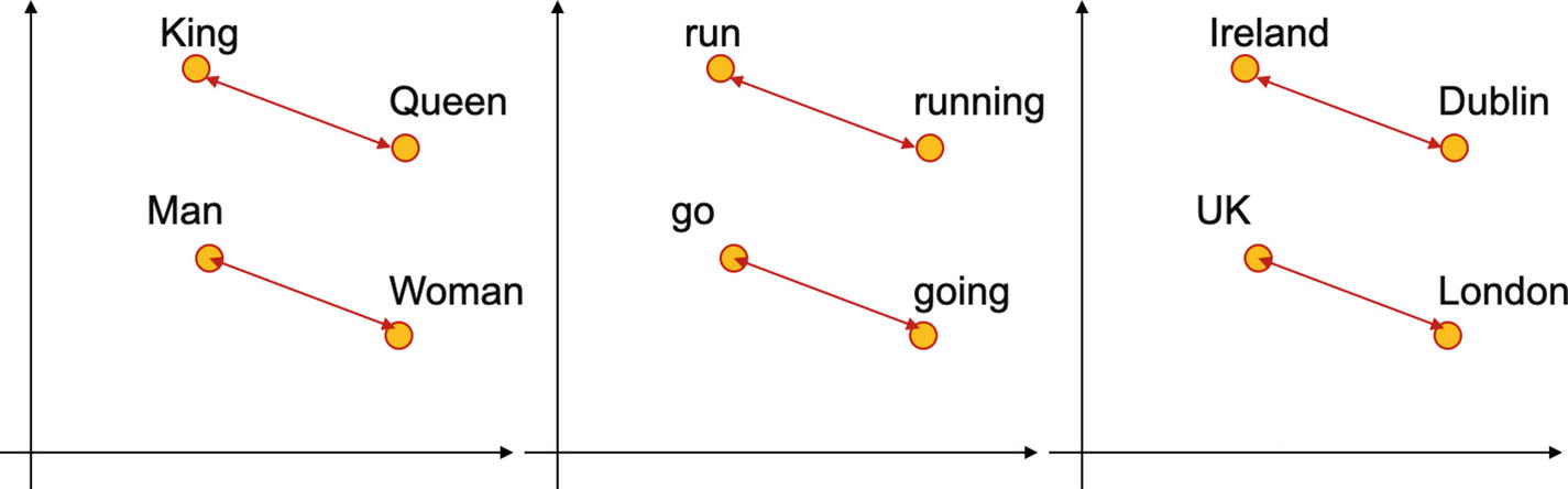
Word embeddings help in finding the contextual relationship between words which are used in the same context and hence improve understanding
In the example shown previously, the relation of “man” to “woman” is like that of “king” to “queen”; “go” to “going” is like “run” to “running”; and “UK” to “London” is like “Ireland” to “Dublin.”
There are two popular word embedding models: Word2Vec and GloVe. Word2Vec provides dense embeddings that understand the similarities between “king” and “queen.” GloVe (Global Vectors for word representations) is an unsupervised algorithm for obtaining representations of words where the training has been performed on aggregated global word-to-word co-occurrence statistics from a corpus.
Both models learn and understand the geometrical encodings or in other words vector representation of their words from the co-occurrence information. Co-occurrence means how frequently the words appear together in the large corpus. The prime difference is that Word2Vec is a prediction-based model, while GloVe is frequency based. Word2Vec predicts the context given a word while GloVe learns the context by creating a co-occurrence matrix on how frequently a word appears in a context. The mathematical details for Word2Vec and GloVe are beyond the scope of this book.
Case study: Customer complaints analysis using word embeddings
We will now use Python and word embeddings to work on the same complaints data we used in the last section.

In the preceding example, we have used word embeddings to create a supervised classification algorithm. This is a very standard and robust process which can be implemented for similar datasets. For accuracy in a text data, data preprocessing holds the key; the cleaner the data is, the better is the algorithm!
Text data is one of the most interesting datasets to work upon. They are not easy to clean and often require a huge investment of time and processing power to create a model. But despite that, text holds the key to very insightful patterns present in the data. We can use text data for multiple use cases and can generate insights which might not be possible from standard structured data sources.
This concludes our discussion on the text data. We will now move to images, which are as interesting and equally challenging. Since images mostly perform better with deep learning, we will be studying building blocks of neural networks to solve supervised learning case studies for images.
Image Data
If the power of conversation is a gift, vision is a boon to us. We see, we observe, we remember, and we recall whatever we have seen. Through our power of vision, we create a world of images. Images are everywhere. Using our cameras and phones, we click photos. We view photos on social media and at online marketplaces. Images are changing the experience we have, the way we shop, the way we communicate, and the way a business can get its customers.
Similar to test data, images can fall under unstructured data categories. An image is made up of pixels. For each colored image, each pixel can have RGB (red, green, blue) values which range from 0 to 255. We can hence represent each image in pixel values (i.e., in the form of matrix) and do the necessary computations on them.
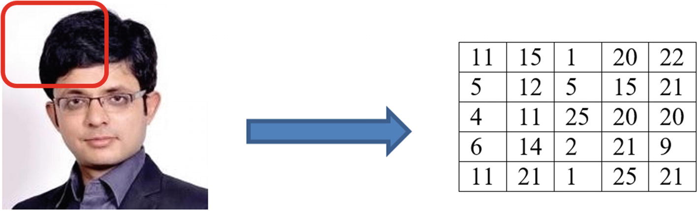
Illustration to show how can an image be represented in a matrix; the numbers are shown only as an example and are not necessarily correct
Images are a very powerful source of information. Image data can be analyzed and used for multiple business use cases, which we will discuss next.
Use Cases of Image Data
Consider this. You want to get a coffee from a coffee vending machine. You go to the machine, and the machine recognizes you, recalls your preferences, and delivers precisely what you wanted. The coffee vending machine has recognized your face and based on your previous transactions has given you the desired flavor. Or the attendance monitoring system at an office uses a facial recognition system to mark attendance instead of swiping cards. Analysis of image data and computer vision are enhancing the capabilities and automating processes everywhere.
- 1.
Healthcare : Image analysis allows us to identify tumors and illnesses from the x-rays, MRIs, and CT scans. The trained ML model can identify if the image is good or bad, which means are there any signs of illness? The solutions can then locate the problem and then the doctors and medical professionals can use the insights generated and focus on the issues. Patients in remote locations can have their images shared with experts and can get a faster response. We use image segmentation and image classification techniques to identify anomalies and perform analysis.
- 2.
Retail industry is harnessing image analysis techniques in a novel way. Customers can upload their pictures of their preferred products like watches, T-shirts, glasses, and so on online and can get a recommendation from the engine. In the background, the online engine will search for similar products and show them to the customer. Moreover, inventory management becomes a lot easier with better image detection techniques. Image segmentation, classification, and computer vision techniques solve the purpose for us.
- 3.Manufacturing: The manufacturing sector employs image analysis techniques in a number of ways:
- a.
Defect identification is done to separate faulty products from the good ones. It can be implemented using computer vision and image classification.
- b.
Predictive maintenance gets improved by identifying the tools and systems which require maintenance. It makes use of image classification and image segmentation techniques.
- a.
- 4.
Security and monitoring: Computer vision allows direct monitoring using a security camera and prevents thefts and crime. The capabilities help in crowd management and crowd control, passenger activity movement, and so on. Live monitoring using cameras allows the security teams to prevent any mishaps. Facial recognition techniques allow us to achieve the results.
- 5.
Agriculture: The field of agriculture is no different. It also makes use of image recognition and classification techniques to identify weeds amid the plants or any type of disease and infection on the plantations. Soil quality can be checked, and the quality of the grain can be improved. Computer vision is really changing the face of one of the oldest occupations of mankind.
- 6.
Insurance : Image analysis is helping the insurance industry by inspecting images from accident sites. Assessment can be made of the damage based on the images from the accident site and claims can be assessed. Image segmentation and image classification drive the solution for the insurance industry.
- 7.
Self-driving cars are a very good example of harnessing the power of object detection. Cars, pedestrians, trucks, signs, and so on can be detected and appropriate action can be taken.
- 8.
Social media platforms and online marketplaces employ sophisticated image recognition techniques to identify the face, features, expressions, product, and so on based on the photos of the user. It helps them to improve the consumer experience, and improve speed and ease of access.
The preceding use cases are only a few of many use cases where image recognition, object detection, image tracking, image classification, and so on are generating out-of-the-box solutions for us. It is propelled by the latest technology stack of neural networks, convolutional neural networks, recurrent neural networks, reinforcement learning, and so on. They push the boundaries as these solutions are capable of processing tons of complex data easily and generating insights from them. We are able to train the algorithms in a much faster way using modern computing resources and cloud-based infrastructure.
But still we have to explore the full potential of images; we have to improve the existing capabilities and enhance the levels of accuracy. A lot of research is going on in this field with several organizations contributing to the advancement of the sector.
Images are a complex dataset to capture and manage. We will now examine the common challenges we face with the images.
Challenges with Image Data
- 1.
Complexity: An image of a car will look different from different angles. Front pose vs. left pose vs. right pose of the same person might look completely different, which makes identification of a person or an object by a machine a difficult process. This level of complexity makes image data tougher to analyze.
- 2.
Size of the dataset: Size of an image is the next challenge we face with image data. An image can easily be in MB, and based on the frequency of generation, the net size of the image dataset can be really huge.
- 3.
Images are multidimensional as compared to any structured data. It also changes as per the image color scale. A multicolored image will have three channels (RGB) and it will increase to the number of dimensions further.
- 4.Unclean data: Images are not always clean. While capturing the dataset itself we face multiple issues. Here are a few of them:
- a.
Blurred images are created if the images are out of focus.
- b.
There can be shadows on the image which makes it unusable.
- c.
Image quality depends on the surrounding lights. If the background light changes, an image will change its compositions.
- d.
Distortions happen in the image due to multiple factors like camera vibrations, or the corners are cut or there are marks (like thumb impressions) on the lens.
- a.
- 5.
Human variability: While capturing the image data, human-generated variance results in different datasets for the same type of problem. For example, if we have to capture the images of crops from a field, different people will capture images from different angles and with different camera modes.
Images are a difficult data set to store and process. Particularly, due to their size, the amount of space required is quite high. We now discuss the image data management process, which concentrates on a few such aspects.
Image Data Management Process
We generate images from multiple sources, and we have to have a concrete data management process for the images. A good system will be able to accept the incoming images, store them, and make them accessible for future analysis. The process of image data management will depend on the design of the system: is it a real-time image analysis project or a batch-processing project? The various sources of images are to be staged, cleaned, and finally stored in a place where they can be accessed as shown in Figure 4-20.

Real-time process and data management for an ML model
In the process diagram shown previously, the term “process” represents the source of image data generation. In the number plate reading case discussed previously, it will be the raw image generated by a camera. These raw images might need to be stored temporarily before they are fed to the compiled ML model. The ML model will generate the prediction about the image. In the preceding case, it will be the car registration number. The prediction and the images, both have to then be stored in the final destination database.

Batch-processing of image data can receive data from a database, make a prediction, and share the results back to the database to be stored
For the batch-processing image analysis system, the “process” will generate the images. Those raw images will have to be stored in a database. Then they are fed to the ML model, which generates the predictions for them. In the preceding case, raw images of the cars will be stored as and when they are generated. They are then fed to the image-processing solution as a batch, which generates the registration number for each car. The predictions and the raw images are then sent back to the database and saved.
A good image data management system should be robust, flexible, and easy to access. The size of the images will play a big role in designing the system. It also defines the cost associated with such a database repository. It is worthwhile to note that such a repository will get consumed very soon, so depending on the critical nature of the business and the domain, we might not save all the images. It is also possible that data which is older than a desired frequency might be deleted from the database.
We will now start with the ML modeling process on image data. And for this, we will start with concepts of deep learning in the next section.
Image Data Modeling Process
- 1.
An image dataset has much greater number of dimensions as compared to structured data, and this makes processing difficult.
- 2.
The background noise in case of images is much higher. There can be distortions, blurring, multiple angles shot, gray-scale images, and so on in the image dataset.
- 3.
The size of the input data is again higher than the structured datasets.
Because of a few of the preceding reasons, we prefer to use neural networks to create the image supervised learning algorithms for us, which we discuss in the next section.
Fundamentals of Deep Learning
Deep learning is changing the way we perceive information. It is enhancing the power of data to new levels. Using sophisticated neural networks, we are able to process many complex datasets, which are many dimensional and are of a great size. Neural networks are truly changing the landscape of ML and AI.
Deep learning has created capabilities which were only a thought a few years ago. In the area of image processing, we are implementing neural networks for image classification, object detection, object tracking, image captioning, semantic segmentation, human pose estimation, and so on. The GPUs and TPUs are increasingly allowing us to push the barriers of processing tons of dataset in no time.
In the following section, we are going to discuss the building blocks of neural networks and will be developing a use case in Python.
Artificial Neural Networks
Artificial neural networks or ANNs are arguably inspired by the functioning of a human brain. When we humans see an object for the first time, we create an image of it in our mind and register it. When the same object comes in front of us again, we are able to recognize it easily. The task, which is too easy for us, is quite difficult for algorithms to understand and learn.
Depth in deep learning represents the number of hidden layers in the neural network. Generally, the higher the number of hidden layers, the greater is the accuracy. But that is true to a certain extent only, and sometimes the accuracy might not increase even with increasing the number of layers.
We train neural networks like we train any ML algorithm—there is an input dataset, we process it, and the algorithm will generate the output predictions for us. A neural network can be used for both regression and classification problems. It can be used for both structured and unstructured data sources. The levels of accuracy by a neural network are generally higher than a classical ML algorithm like regression, decision tree, and so on. But that might not always be true.
The biggest advantage we have with a neural network is its ability to process complex data like images and videos. Then, recall for classical ML algorithms we choose the significant variables. In the case of neural networks, it is the responsibility of the network to pick the most significant attributes from the data.

A neural network has input layer, hidden layers, and output layer
- 1.
Neuron: A neuron is a foundation of a neural network. All the calculations and complex processing take place inside a neuron only. It expects an input data like image and will generate an output. That output might be consumed by the next layer in the network or might be used to generate the final result. A neuron can be represented as shown in Figure 4-23. Here, x0, x1, and x2 represent the input variables, and w0, w1, and w2 are their respective weights. “f” is the activation function and “b” is the bias term.
A neuron receives input from the previous layers and then based on the conditions set, decides whether it should fire or not. Simply put, a neuron will receive an input, perform a mathematical calculation on it, and then based on the threshold set inside itself will pass on the value to the next neuron.
During the training of the ML model or the network in this case, weights and bias terms get trained and we get the most optimized value. We will be discussing the training mechanism and activation term in the next section.

Basic structure of a neuron showing inputs, weights, activation function, and an output
- 2.
Input Layer: As the name signifies, input layer accepts the input data. It can be in the form of images (raw or processed). This input layer is the first step in the network.
- 3.
Hidden Layer: Hidden layers are the most important segment in a neural network. All the complex processes and mathematical calculations take place in the hidden layer only. They accept the data from the input layer, process it layer by layer, and then feed it to the output layer.
- 4.
Output Layer: Output layer is the last layer in a neural network. It is responsible for generating the prediction, which can be a continuous variable for a regression problem or a probability score for a supervised classification problem.
With these building blocks of a neural network, in the next section we will discuss the other core elements of a network, which are activation functions.
Activation Functions
Activation functions play a central role in training of a neural network. An activation function’s primary job is to decide whether a neuron should fire or not. It is the function which is responsible for the calculations which take place inside a neuron.
The activation functions are generally nonlinear in nature. This property of theirs allows the network to learn complex behaviors and patterns.
- 1.
Sigmoid activation function : Thist is a bounded mathematical function as shown in Figure 4-24. The range of a sigmoid function is between 0 and 1. The function is S shaped and has a non-negative derivative function.
Mathematically, a sigmoid function is
 (Equation 4-2)
 Figure 4-24
A sigmoid function has an S-like shape
It is usually used for binary classifications and in the final output layer of the neural network. But it can be used in the hidden layers of the network too.
- 2.
tanh activation function : Tangent hyperbolic function or tanh is a scaled version of the sigmoid function as visible in Figure 4-25. As compared to the sigmoid function, tanh is zero centered. The value ranges between –1 and +1 for tanh function.
Mathematically, tanh function is given by
 (Equation 4-3)tanh activation function is generally used in the hidden layers of the neural network. It makes the mean closer to zero, which makes the training easier for the network.
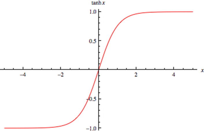 Figure 4-25
A tanh function is centered at zero
- 3.
ReLU activation function : Perhaps the most popular of the activation functions is the ReLU activation function. ReLU is a rectified linear unit and is shown in Figure 4-26.
F(x) = max (x,0) gives the output as x if x>0; otherwise, the output is 0.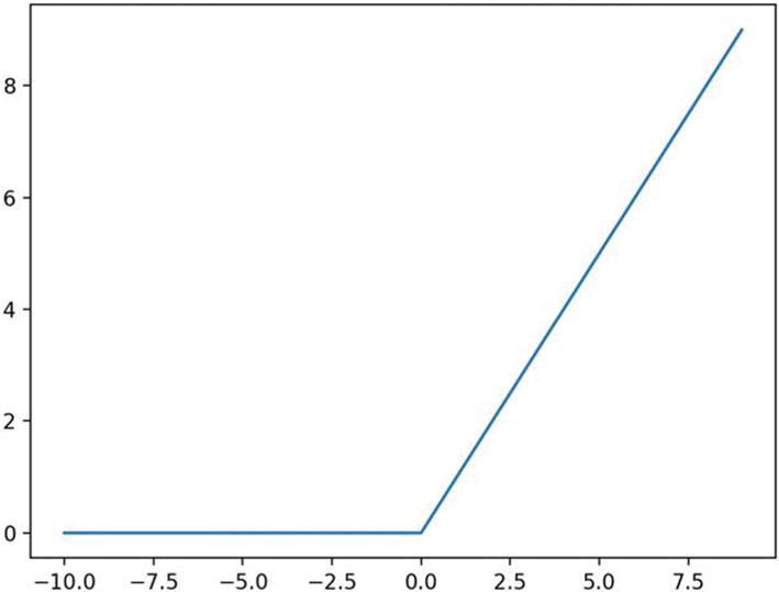 Figure 4-26
A ReLU function
ReLU is a very simple function to compute, as visible from the simple mathematical function. It makes ReLU very easy to compute and very fast to train. It is used in the hidden layers of the network.
- 4.
Softmax function : The softmax function is used in the final layer of the network used for classification problems. It is used for generating the predictions in the network. The function generates probability scores for each of the target classes, and the class which receives the highest probability is the predicted class. For example, if the network is aimed to distinguish between a cat, dog, a horse, and a tiger, the softmax function will generate four probability scores. The class which receives the highest probability is the predicted class.
Activation functions play a central role in training the network. They define the training progress and are responsible for all the calculations which take place in various layers of the network. A well-designed network will be optimized and then the training of the model will be suitable to be able to make the final predictions. Similar to a classical ML model, a neural network aims to reduce the error in predictions, also known as the loss function, which we cover in the next section.
Loss Function in a Neural Network
We create an ML model to make predictions for the unseen dataset. An ML model is trained on a training dataset, and we then measure the performance on a testing or validation dataset. During measuring the accuracy of the model, we always strive to minimize the error rate. This error is also referred to as loss.
Formally put, loss is the difference between the actual values and predicted values by the network. For us to have a robust and accurate network, we always strive to keep this loss to the minimum.
We have different loss functions for regression and classification problems. Cross-entropy is the most popular loss function for classification problems, and mean squared error is preferred for regression problems. Different loss functions give a different value for the loss and hence impact the final training of the network. The objective of training is to find the minimum loss, and hence the loss function is also called objective function.
binary_crossentropy can be used as a loss function for binary classification model.
The neural network is trained to minimize this loss and the process to achieve it is discussed next.
Optimization in a Neural Network
During the training of the neural network, we constantly strive to reduce the loss or error. The loss is calculated by comparing the actual and predicted values. Once we have generated the loss in the first pass, the weights have to be updated to reduce the error further. The direction of this weight update is defined by the optimization function.
Formally put, optimization functions allow us to minimize the loss and reach the global minimum. One way to visualize the optimization is as follows: imagine you are standing on top of a mountain. You have to reach the bottom of the mountain. You can take steps in any direction. The direction of the step will be wherever we have the steepest slope. Optimization functions allow us to achieve this. The amount of step we can take in one stride is referred to as the learning rate.
- 1.
Gradient descent is one of the most popular optimization functions. It helps us achieve this optimization. Gradient descent optimization is quite fast and easy to implement. We can see gradient descent in Figure 4-27.

Gradient descent is used to optimize the loss for a neural network
- 2.
Stochastic gradient descent or SGD is a version of gradient descent only. As compared to its parent, it updates the parameters after each training example, that is, after the loss has been calculated after each training example. For example, if the dataset contains 5000 observations, gradient descent will update the weights after all the computations are done and only once, whereas SGD will update the weights 5000 times. While this increases accuracy and decreases computation memory requirements, it results in overfitting of the model too.
- 3.
Minibatch gradient descent is an improvement over SGD. It combines best of the gradient descent and SGD. In minibatch gradient descent, instead of updating the parameters after each training example, it updates them in batches. It requires a minimum amount of computation memory and is not prone to overfitting.
- 4.
There are other optimization functions too like Ada, AdaDelta, Adam, Momentum, and so on which can be used. The discussion of these optimizers is beyond the scope of this book.
Adam optimizer and SGD can be used for most problems.
Optimization is a very important process in neural network training. It makes us reach the global minima and achieve the maximum accuracy. Hence, due precaution is required while we choose the best optimization function.
There are a few other terms which you should be aware of, before we move to the training of a network.
Hyperparameters
A network learns quite a few parameters itself by analyzing the training examples but a few parameters are required to be fed. Before the training of the neural network commences, we set these parameters to initiate the process. These variables determine the structure of the network, the process, variables, and so on which are used in the final training. They are referred to as hyperparameters .
We set a number of parameters like the learning rate, the number of neurons in each layer, activation functions, number of hidden layers, and so on. We also set the number of epochs and batch size. The number of epochs represents the number of times the network will analyze the entire dataset completely. Batch size is the number of samples the network analyzes before updating a model parameter. A batch can contain one or more than one samples.
Simply put, if we have a training data size of 10,000 images, we set batch size as 10 and number of epochs as 50; this means that the entire data will be divided into 10 batches each having 1000 images. The model’s weight will be updated after each of those 10 batches. This also means that in one epoch 1000 images will be analyzed 10 times, or in each epoch the weights will be updated 10 times. The entire process will run 50 times as the number of epochs is 50.
There are no fixed values of epoch and batch-size. We iterate, measure the loss and then get the best values for the solution.
But training a neural network is a complex process, which we will discuss next. There are processes of forward propagation and backward propagation which are also covered in the next section.
Neural Network Training Process
A neural network is trained to achieve the business problem for which the ML model is being created. It is a tedious process with a lot of iterations. Along with all the layers, neurons, activation functions, loss functions, and so on, the training works in a step-by-step fashion. The objective is to create a network with minimum loss and optimized to generate the best predictions for us.
- 1.
TensorFlow: It is developed by Google and is one of the most popular frameworks. It can be used with Python, C++, Java, C#, and so on.
- 2.
Keras: It is an API-driven framework and is built on top of TensorFlow. It is very simple to use and one of the most recommended libraries to use.
- 3.
PyTorch: PyTorch is one of the other popular libraries by Facebook. It is a very great solution for prototyping and cross-platform solutions.
- 4.
Sonnet: It is a product by DeepMind and is primarily used for complex neural architectures.
There are many other solutions like MXNet, Swiftm Gluon, Chainer, and so on. We are using Keras to solve the case studies in Python.
Now we will start examining the learning of a neural network. Learning or training in the case of a network refers to finding the best possible values of the weights and the bias terms while keeping an eye on the loss. We strive to achieve the minimum loss after training the entire network.
The major steps while training a neural network are as follows:
Step 1: In the first step, as shown in Figure 4-28, the input data is passed on to the input layer of the network. The input layer is the first layer. The data is fed into a format acceptable by the network. For example, if the network expects an input image of size 25×25, that image data is changed to that shape and is fed to the input layer.
Next, the data is passed and fed to the next layer or the first hidden layer of the network. This hidden layer will transform the data as per the activation functions associated with that particular layer. It is then fed to the next hidden layer and the process continues.

Step 1 in the neural network showing the input data is transformed to generate the predictions
Step 2: Now we have achieved the predictions from the network. We have to check if these predictions are accurate or not and how far the predicted values are from the actual values. This is done in this step as shown in Figure 4-29.
Here, we compare the actual and predicted values using a loss function and the value of loss is generated in this step.
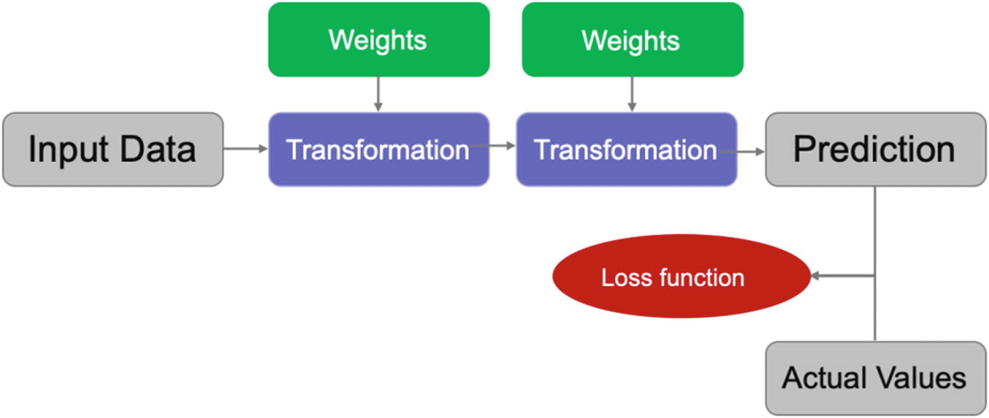
Loss is calculated by comparing the actual and predicted values
Now we have generated the perceived loss from the first iteration of the network. We still have to optimize and minimize this loss, which is done in the next step of training.
Step 3: In this step, once the loss is calculated, this information travels back to the network. The optimization function will be changing the weights to minimize this loss. The respective weights are updated across all the neurons, and then a new set of predictions are generated. The loss is calculated again and again the information travels backward for further optimization, as shown in Figure 4-30.
This travel of information in a backward direction to optimize the loss is referred to as backward propagation in a neural network training process.
Backward propagation is sometimes called the central algorithm in deep learning.
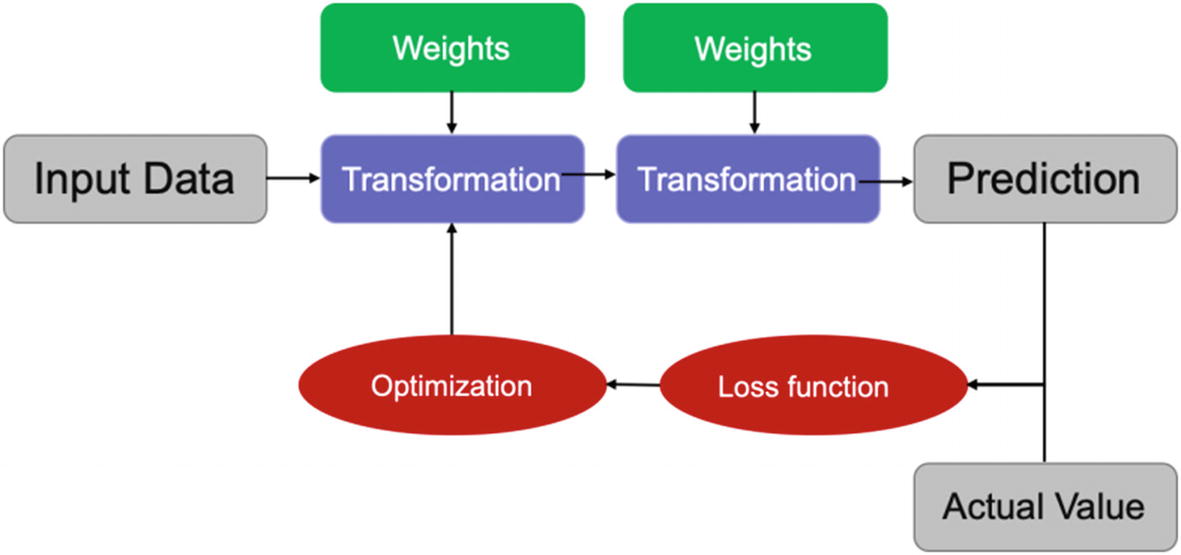
The optimization is done to minimize the loss and hence reach the best solution
This is the process for a network to train itself and generate a compiled model for us. The training for a neural network is also referred to as learning of a network. Formally put, learning of a network refers to finding the most optimal values and best combinations of weights for all layers of the network.
Initially, all the weights are initialized with some random values. The network makes the first prediction, and due to obvious reasons, the loss or the error in the first pass will be quite high. Now, the network encounters new training examples and based on the loss calculated the weights are updated. The backpropagation plays the central role here by acting as a feedback loop. During the process of training the network, these weights are updated during each iteration. The direction of iteration is defined by the gradient of the loss function which allows us to move in the direction to minimize the loss. Once the loss can no longer be decreased, we can say that the network is trained now.
We will now learn how a neural network is trained by creating two use cases in Python: one on structured data and another for images.
Case Study 1: Create a Classification Model on Structured Data
We are using the diabetes data set. The objective is to diagnostically predict if a patient has diabetes or not based on certain diagnostic measurements. The code and dataset are uploaded at Github.


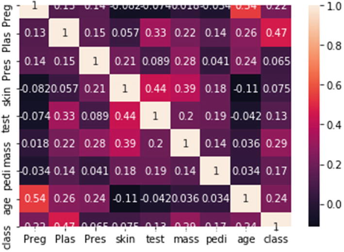

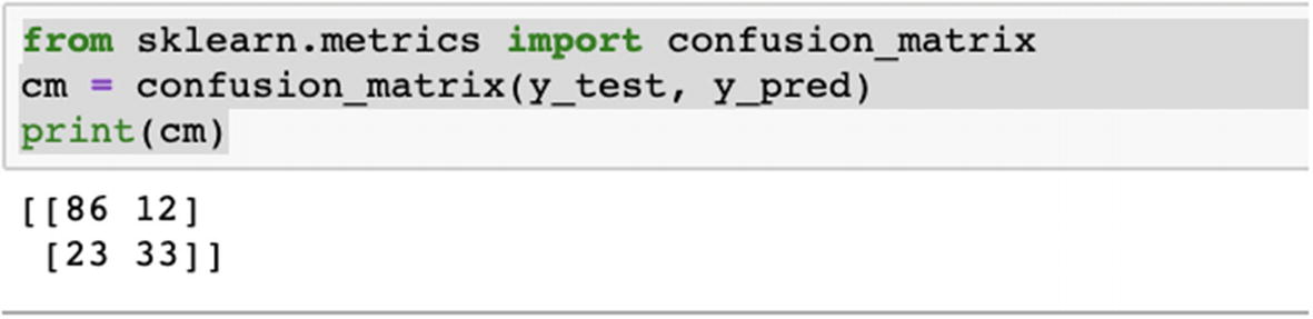
Here we can deduce that the model has an accuracy of 77.27%.
- 1.
Increasing the complexity of the network by adding one or two more layers.
- 2.
Testing with different activation functions. We have used sigmoid; you can use tanh.
- 3.
Increasing the number of epochs and checking the performance.
- 4.
Preprocessing the data better and then again checking the performance over the revised dataset.
Case Study 2: Image Classification Model
We will develop an image classification model on fashion MNIST dataset. It has 70,000 grayscale images in 10 different categories. This dataset is used for image classification problems and is a standard dataset to be used. It comes prebuilt with Keras and can be loaded easily.
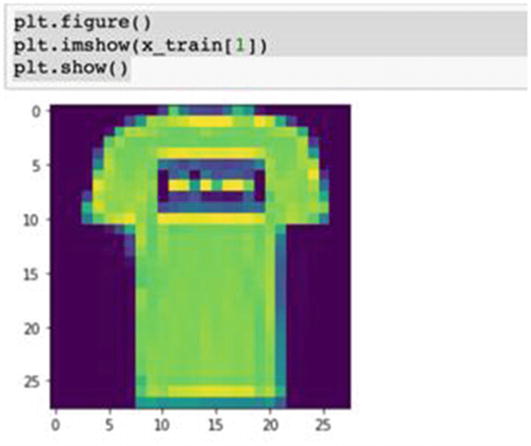
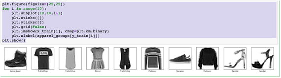
Here, the input image shape is 28,28. The flatten layer transforms the format of images to 28×28. It only reformats the data and has nothing to learn. Next is the layer that has ReLU as an activation function and 256 neurons. The last layer has 20 neurons and returns a logit array indicating if an image belongs to one of the ten classes we are training upon.
The parameters are loss functions to measure how accurate the model is during training. The optimizer determines how the model is updated based on the data it sees and its loss function. We are using accuracy to monitor the training and testing steps.
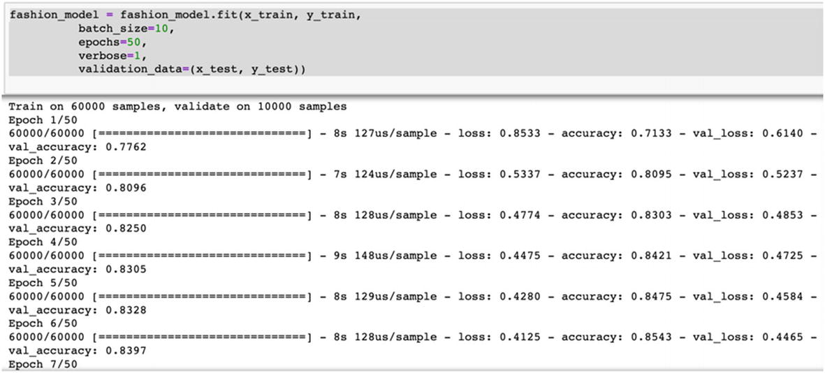
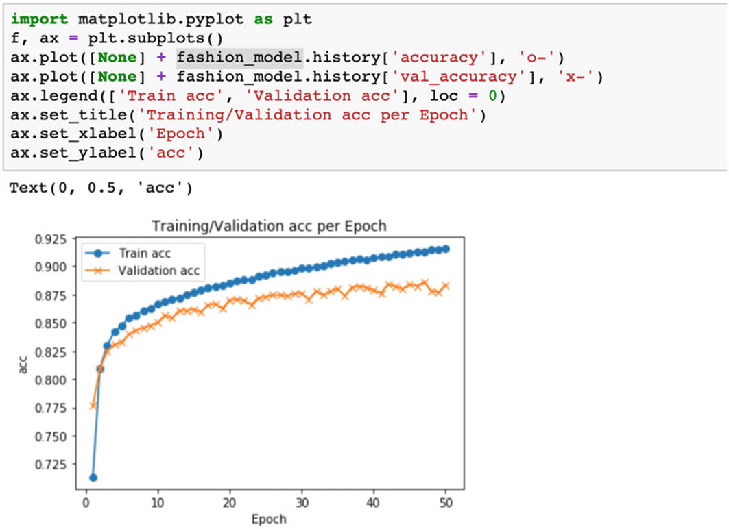
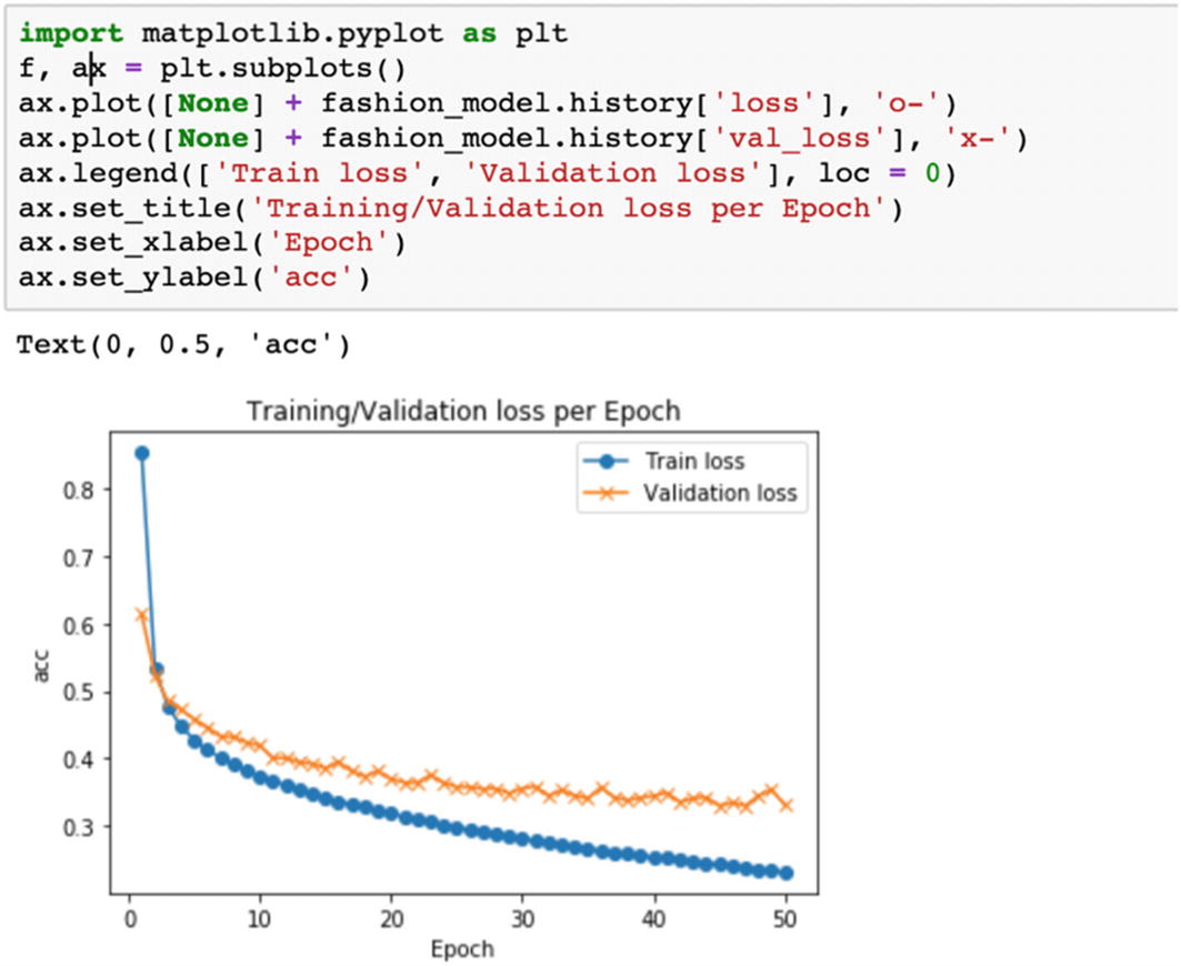
The test accuracy of the model is 89.03%. Like the last case study, you are advised to iterate by changing the network architecture by adding layers and neurons, and by measuring the performance with different values of epoch, batch_size etc.
We have thus implemented two use cases for structured and unstructured data using deep learning.
Deep learning is the power which allows us to improve capabilities further. For unstructured datasets, neural networks are leading the path in getting solutions which were unheard of before. Advanced neural networks like convolutional neural networks, recurrent neural networks, long short term memory (LSTM), GRU, and so on are doing wonders in every field. We can now detect cancer better, enhance security systems, improve agricultural yields, reduce shopping time, use facial features for allowing or restricting users—the use cases are plenty. And across all the domains, we can feel the ripple effect of deep learning.
With this, we are coming to the end of the fourth chapter of the book. Let’s summarize the chapter now.
Summary
This chapter is quite special as it works with advanced concepts. But these advanced concepts are built on top of the basics we have created in the initial chapters. These advanced concepts and algorithms are the need of the hour. With better processing power and enhanced systems, we can implement faster solutions. The required computation power, which is now available, was not in existence a decade back. We now have GPUs and TPUs at our disposal. We now can store and manage terabytes or petabytes of data. Our data collection strategy has improved a lot. We can collect real-time data in a much more structured way. Our data management tools are now not limited to standalone servers only, but have expanded to cloud-based infrastructures. It provides tools and confidence to implement much more advanced ML-based techniques to further improve the capabilities.
At the same time, we cannot undermine the importance of algorithms studied in the previous chapters. Linear regression, decision tree, knn, naïve Bayes, and so on are the foundation of ML algorithms. They are still a preferred choice for shortlisting significant variables. These algorithms set up a benchmark of performance. Ensemble techniques of bagging and boosting then enhance the capabilities further. Hence, before starting with boosting or bagging algorithms, we should always test and benchmark the performance with the base algorithms.
With the advent of deep learning, we are able to process much more complex datasets. Deep learning gives an extra push to the performance. But for processing deep learning algorithms, we require better hardware systems. Cloud-based infrastructures offer good services in this case. We can deploy our code in Google Colaboratory and run the code, thereby utilizing the processing power of the servers.
With this, we have discussed the supervised learning algorithms within the scope of the book. In Chapter 1, we introduced ML. In Chapters 2 and 3, we examined regression and classification algorithms. In this fourth chapter we studied advanced algorithms like boosting, SVMs, and deep learning models and worked on both structured and unstructured data. In the next chapter, which is the last chapter of the book, we will examine the end-to-end process of a model’s life—from scratch to maintenance.
You should now be able to answer the following questions.
Question 1: What are different versions of gradient boosting available?
Question 2: How does an SVM algorithm distinguish between classes?
Question 3: What are the data preprocessing steps for text data?
Question 4: What are the various layers in a neural network?
Question 5: What is the function of a loss function and an optimization function in a neural network?
Question 6: Take the datasets used in the last chapter for classification problems and test the accuracy using SVM and boosting algorithms.
Question 7: Download the breast cancer classification data from https://www.kaggle.com/uciml/breast-cancer-wisconsin-data. Clean the data and compare performance of random forest and SVM algorithms.
Question 8: Get the Amazon reviews dataset from https://www.kaggle.com/bittlingmayer/amazonreviews. Here the problem is to analyze customer reviews on Amazon as input text and output ratings as the output label. Clean the text data using the techniques discussed and create a classification algorithm to make predictions.
Question 9: Download the movie reviews text dataset from http://ai.stanford.edu/~amaas/data/sentiment/ and create a binary sentiment classification problem.
Question 10: Get the images from https://www.kaggle.com/c/dogs-vs-cats and create a binary image classification solution using neural network to distinguish between a dog and a cat.
Question 11: Extend the preceding problem to multiclass problem by downloading the data from https://www.cs.toronto.edu/~kriz/cifar.html.
- (1)
- (2)
- (3)
- (4)
- (5)