
This chapter will deal with the quality of the data produced by experimental measurements. To use data, it must be reproducible and validated. Experiments and experimental setups must be able to generate reproducible data that can also be reproduced by other investigators using the same experimental technique. Once data can be replicated it can be validated or tested for veracity or truthfulness. A simple technique for validating a weighing instrument is to weigh a well-known defined weight standard. A second method for validating data is to use a different measurement technique to confirm the original observation. A mercury-in-glass temperature determination could be verified by either a thermistor or a thermocouple reading.
Quality Assurance and Control
Repetitive measurement techniques such as weighing, measuring a temperature, or measuring relative humidity that are part of another experimental process should be subjected to a quality assurance, quality control procedure so the data generated by the experimental process of which they are a part can be monitored and ultimately validated. The quality of repetitive measurements can be monitored through the application of statistical process control (SPC) in the form of control charting.

The Gaussian distribution
The shape of the plot in Figure 7-1 is a “normal” or “Gaussian” distribution. Averaging the large number of values calculates the mean value, M or  . The standard deviation of the data set can then be calculated by well-known mathematical techniques. A standard deviation is a measure of the variation or dispersion of a set of data. The value is represented by σ. The mean and standard deviation are calculated with the two equations in the following section. In Figure 7-1, the arrow represents the points at which the probability of finding values in the data set represented by the given distribution curve in red that are 10 or more above or below the mean value of M is very small. The majority of values lie between + or – 3σ. Because the probability of there being a value of the known data set outside of the 3σ limit is very small, it is possible to set up a “3σ” control chart. Repetitive measurements of the same parameter value should all cluster around the mean value. The probability of the measured value at hand being more than twice or three times the standard deviation of the mean becomes increasing small, and hence if such a value occurs repetitively, then the system is said to be “out of control.”
A statistical rule of thumb (Chebyshev’s Theorem) states that 68 percent of the dataset will lie within one standard deviation of the mean, 95 percent within 2, and 99.7 percent within 3.
Control charts are dynamic graphic displays used to document how a process changes over time. Data values are plotted in a sequential time order about a central horizontal axis defining the median value of the data. Under normal conditions the data being plotted should be randomly scattered above, below, and occasionally on the median value or center line. To aid in visualizing a randomly distributed data set and detecting values not in conformance with the random distribution assumption, six additional lines parallel to the median axis at +/- 1σ, +/- 2σ, and +/- 3σ are added to the chart.
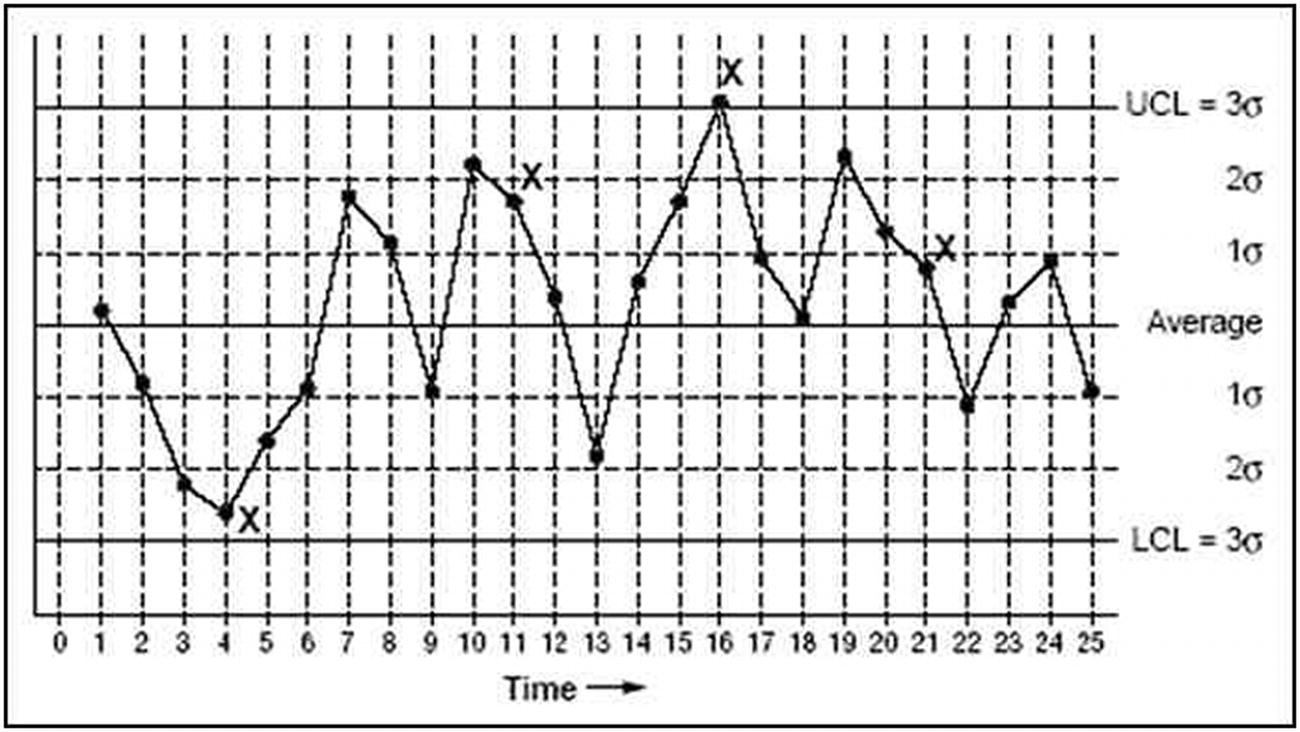
On a 3σ control chart, the top and bottom lines are referred to as the upper and lower control limits that have been determined from validated historical data collected prior to the construction of the control chart.
Consecutive data points falling within the upper and lower control limits indicate that the data being generated are consistent and are referred to as being “in control.” If data points are outside of the control limits, they are unpredictable, and hence the measurement system is “out of control.”
There are a large number of problems that can be detected with control charts besides the “in or out” of control condition. Consecutive data points should not drift up or down in a predictable trend. The data points should be randomly distributed above and below the median axis. An experimenter encountering a deviation from the expected performance of the measurement system must find the source of the deviation and correct the method being used to collect or generate the data.
A typical application for a control chart can involve validating the performance of a weighing device before it is used in an actual weighing operation as part of a research investigation. Prior to a daily or “when needed” weighing operation, a reference standard whose weight value is well known is measured. The newly determined weight value is entered into the control-charting operation. If the newly entered value is acceptable, the device can be used for weighing operations. At the end of the experiment or at the end of the day, the reference weight is re-weighed and the fresh value entered into the control-chart program. If the end-of-experiment or end-of-day value is acceptable, then all the weight determination values conducted between the two “in control” determinations of the reference weight can be deemed valid.
Error Analysis
It has been realized for hundreds of years that even very carefully made measurements of the same parameter do not produce the same results. As is illustrated in Figure 7-1, multiple repetitions of a reliable measurement technique always produce a collection of numbers that conform to a bell-shaped pattern when the mean value and the individual numerical differences of the data set of numbers are calculated and plotted.

A common statistical notation representing a mean or average value is to place a small dash or “bar” over the variable representing the value obtained when the sum of all the values is divided by the number of values summed. The ∑ notation (“sigma” notation) to the right is read as “the sum of the variables Xk for all k values from k = 1 to k = N.
As noted, the tendency of a set of numbers to conform to the pattern seen in Figure 7-1 was first noted by the mathematician Gauss and is called a Gaussian distribution. The pattern is also known as a “normal” distribution.

In statistics, N or n is usually the number of data points in the set, and the squared term (x – mean) is the difference between each individual x value and the mean value of the set. The squaring operation converts all positive- and negative-difference values into positive numbers whose squared value is then summed as noted by the ∑ notation. The summed value is then averaged by dividing by n—the number of data points prior to having the square root extracted of the averaged squares—to return a result value in the original scale. If a measurement is repeated many times, at least 68 percent of the measured values will fall in the range +/- 1σ of the mean. (In statistical terms, the preceding formula is often stated as “the standard deviation is the square root of the variance.” The variance is the quantity under the root sign. The statistics discussed thus far pertains to only a single set of data obtained from one experiment. If the data under consideration is part of a larger data set, the experimenter must consult a textbook on statistics to obtain the correct formulas for dealing with a subset of a larger population.)
A standard deviation can be thought of as the average difference between the data values and the mean or as the dispersion of the data around the mean. Experimental development programs are often focused on decreasing the value of the standard deviation in the results of a measurement system or in the variations of a product created by a process.
A small value of a standard deviation, however, does not ensure the accuracy of a set of measurements or determinations. Errors are divided into two categories termed random and systematic. Random errors are inherent in all measurements. Systematic errors have an identifiable cause.
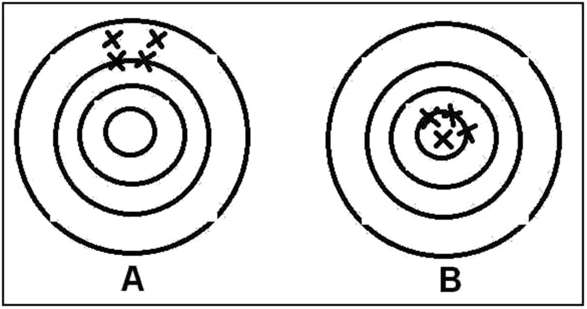
A dart board analogy for precision and accuracy
The scatter within each grouping is representative of the inherent random error that occurs within all measurements. The high grouping in A can be said to have a systematic error. There is no prescribed way to find systematic errors. All the possible sources of a systematic error must be considered or examined and small experiments conducted to see if the suspect sources are active. The ultimate goal of the process is to reduce systematic errors to values less than the random errors in the determination. To reduce the systematic error in A, a longer flight time for the darts could be implemented by having the player step back from the board.
Accuracy is most often assessed with reference standards. Standards are available for virtually any measurement, such as for weights, lengths, temperatures, chemical compositions, and as methods to ensure uniformity in procedures conducted at different locations and times. Standards are provided by organizations such as the Canadian Standards Association (CSA Can.), the National Institute for Standards and Technology (NIST USA), and the International Standards Organization (ISO UN) of the United Nations.
An often overlooked aspect of the reporting of experimental data is the use of significant figures. The accepted convention in reporting experimental errors is that only one uncertain digit should be used.
Calculations using numbers with differing levels of significant figures must always generate results with no more significant figures than the lowest found in the entries entered into mathematical formulations.
Many of the data variations to be expected in the values collected during experimental work can be conveniently demonstrated using digital multimeters and resistors.

Components for measuring data variation with resistors and a sensitive DMM
Repetitive High-Sensitivity Resistance Measurements
- |
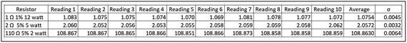
From the table, it seems that the largest dispersion is in the device with the highest resistance value and smallest wattage rating. The smallest device also took the longest time for the display to stabilize. There are several hypotheses that may account for the observations derived from the reproducible data. The time to stability may be directly proportional to the physical size or thermal masses of the different-sized resistors, or it could be hypothesized that the three different resistor types have different resistive core materials that respond differently to electrical excitation.
In addition to the inherent random spreading seen in measurements of the same parameter by the same technique, a number of additional sources of variation are encountered in experimental work.
Different instruments measuring the same parameter will produce variations in the measured results. The repetitive manufacturing of devices with a nominal value or dimension produces variations in the individual unit values.
To illustrate some of the conventions used in reporting experimental data and demonstrating sources of error and variation, a second table of numerical values for the measured resistance of a set of resistors was collected. Ten element samples of 5% tolerance, 1/8 W resistors, spanning five orders of magnitude from 10 Ω to 100 kΩ were measured for their actual resistance with four different digital multimeters.
The 1 MΩ ten-element population differed from the bulk of the experimental subjects in that although each member was a nominal 1/8 W, 5% unit, the subjects were from two additional manufacturers.
Resistance Measurement Data Set
- |

Four different meters were used to measure each of the ten-element resistor sets. The Circuit-Test is a low-cost, four-digit, basic volt, ohm, ampere meter for instrument and lab equipment servicing ($20 CDN). The Velleman DVM890C is a 3½-digit meter with numerous additional functions for capacitance, thermocouples, and other lab-oriented measurements ($50 CDN). The Extech Ex505 is an industrial-grade, autoscaling multimeter with a basic 0.5% accuracy and numerous additional measuring features ($150 USD). The Siglent SDM3055 displayed in Figure 7-4 is a research-grade benchtop meter with a 5½-digit display ($600 CDN). (½-digit notation describes a display in which the most significant digit of the display can be either a 1 or a 0. The remaining number of digits can display digital values from 0 to 9. A 3½-digit display can thus represent a maximum value of 1.999 and any value below that. All ½-digit meters with scale switches are indexed in multiples of two to accommodate the upper 1.999 display limit.)
Recall that digital multimeters are built around high input impedance ADCs that measure voltages. Different meters use different techniques to measure the voltage directly or through precision resistors for resistance and current determinations. ADCs are available in different operational formats with higher digital resolutions, and usually the more precise and accurate measurement circuitry is more expensive to implement.
As can be seen in the 10 Ω measurement data, the lowest standard deviations are seen because the sensitivity of the measurements being made may not be sufficient to see the natural inherent variation that exists in all measurements along with the variation in resistance due to manufacturing.
Note that by convention the number of significant figures recorded is increased by 1 when the average value is reported.
Examination of the data for the 1000 Ω specimens shows the standard deviation σ being returned in the same range or format as the population entries. The Circuit-Test meter uses a four-digit, whole-number display for values less than 9999, while the other meters change display format.
Low-Cost Meter Comparison to High-Resolution Benchtop Meter
- |

Calibration and Curve Fitting
In numerous presentations of tabulated data in this book, a line has been drawn on the plotted data along with an equation and a correlation coefficient. Most of the data has been used to create a straight line that can be used to easily interpolate or calculate values not actually measured in the initial or calibration procedure. The statistical technique used to calculate the straight lines is known as a least squares fit.
The least squares fit is defined as follows: “A method of determining the curve that best describes the relationship between expected and observed sets of data by minimizing the sums of the deviation between observed and expected values.” In very simplified terms, the line is the best fit to the scatter in the data set. The R2 term is called the correlation coefficient and is a measure of how well the equation fits the data. A perfect fit in which all the data points fall on the line would have a correlation coefficient of 1.
There are a number of curve-fitting statistical mathematical operations built into the spreadsheets available today. A textbook on statistical methods is best consulted before the experimenter unfamiliar with these methods applies them to a problem at hand.
Summary
All replicated measurements made of any quantity have a naturally occurring inherent variability in their measured values that when analyzed statistically and plotted form a Gaussian or normal bell-shaped distribution.
Three σ quality-control charts use the inherent variability to monitor the validity of the values generated by the measurement system at hand.
Accuracy, precision, and random and systematic errors are discussed and demonstrated, with the results obtained from a series of resistance measurements.
Systematic errors are demonstrated in Chapter 8 when the problems and limitations of using the USB for both power and transmission of sensitive experimental data are considered.