© The Author(s), under exclusive license to APress Media, LLC, part of Springer Nature 2021
M. Cywiak, D. CywiakMulti-Platform Graphics Programming with Kivyhttps://doi.org/10.1007/978-1-4842-7113-1_8

8. Stereoscopic 3D Plots

Moisés Cywiak1   and David Cywiak2
(1)
Leon, Guanajuato, Mexico
(2)
Queretaro, Mexico
 
In this chapter, we describe the basic elements for constructing stereoscopic 3D plots of analytical functions. A screenshot of this program obtained from an Android cell phone is shown in Figure 8-1.
../images/510726_1_En_8_Chapter/510726_1_En_8_Fig1_HTML.jpg
Figure 8-1

Screenshot of the program running in an Android cell phone

The functionality of the buttons is the same as in Chapter 7.

8.1 Creating the Function, Coordinates, and Mesh

The procedures to create the function, the coordinates, and the mesh are described in Chapter 7. The code is shown in Listing 8-1.
P=0.5; # Function at z=D/2
N=40;  #Number of pixels for representing the function
#Arrays for filling function values
x=np.zeros(N+1);
z=np.zeros(N+1); y=np.zeros( (N+1,N+1) );
# Mesh
x1=np.zeros( (N+1,N+1) );
y1=np.zeros( (N+1,N+1) ); z1=np.zeros( (N+1,N+1) );
L=130;  r0=L/5; #L=Gaussian x-z scale. r0= semi-width
XG0=0; ZG0=P*D;
Amplitude=130; #Vertical scale
for n in range (0,N+1): #Filling the x-z axes
    x[n]=(n-N/2)/N*L;
    z[n]=(n-N/2)/N*L;
for n in range(0,N+1): #Filling function pixels
    for m in range(0,N+1):
        y[n][m]=Amplitude*np.exp(- (x[n]**2
                                +z[m]**2)/r0**2 );
Scale_x=1; Scale_y=1; Scale_z=1;
for n in range (0,N+1):
    for m in range(0,N+1):#Filling Mesh
        x1[n][m]=Scale_x* x[n];
        z1[n][m]=Scale_z*z[m]+ZG0;
        y1[n][m]=Scale_y*y[n][m];
Listing 8-1

Creating the Mesh and the Discrete Function

As mentioned, this code is analogous to the code described in Chapter 7.

8.2 Creating Two Images for the Stereoscopic Effect

To produce the stereoscopic effect, we need to project the function onto two images using two points of projections that are slightly displaced horizontally. We use the parameters shown in Listing 8-2 for this purpose.
D=2000;
#Coordinates of the first point of projection.
VX1=-60; VY1=600; VZ1=0;
#Coordinates of the second point of projection.
VX2=60; VY2=600; VZ2=0;
P=0.5; # Percentage value of D; 50% places the function at z=D/2;
Listing 8-2

Setting Parameters for the Stereoscopic View

As in previous chapters, the parameter D is the distance from the plane of projection to the screen. The VX1 and VX2 parameters represent the horizontal coordinates of the point of projection and are displaced between them. The rest of the coordinates are given by VY1=VY2 and VZ1=VZ2. The P parameter represents a percentage of the distance, D, at which the function is placed. For the stereoscopic view, we will set P=0.5 to place the function in the middle, between the plane of projection and the screen.

Initialize(B, *args) is in charge of calculating the dimensions of the screen and of creating two PIL images with appropriate dimensions. These images are PilImage1 and PilImage2. Additionally, two drawing instances for the images are created, Draw1 and Draw2, to allow us to draw lines and text in the images. When the program starts, the 3D Images text is shown. Initialize(B, *args) is shown in Listing 8-3.
def Initialize(B, *args):
        global W,H, XC,YC;
        global PilImage1,PilImage2, Draw1,Draw2;
        #P= Percentage of D distance
        global P, Amplitude;
        W,H=B.ids.Screen1.size;
        XC=int (W/2)+0;
        YC=int(H/2)+60;
        PilImage1= Image.new('RGB', (W-10, H-10),
                                 (60, 70, 30));
        Draw1 = ImageDraw.Draw(PilImage1);
        PilImage2= Image.new('RGB', (W-10, H-10),
                                 (60, 70, 30));
        Draw2 = ImageDraw.Draw(PilImage2);
        Font = ImageFont.truetype('Gargi.ttf', 70);
        Draw1.text( (30,200), "3D Images",
                    fill =(255,0,0,1), font=Font);
        Draw2.text( (50,200), "3D Images",
                    fill =(0,255,255,1), font=Font);
        ShowScene(B);
Listing 8-3

Code Initiating Variables When the Program Starts

We need a third image, which we will name PilImage3, to store the result of bitwise ORing the left and right images. The ShowScene(B) function creates this array.

8.3 Drawing the Plot

GraphFunction(VX, VY, VZ, Which) is in charge of drawing the plot. The Which parameter selects the image to be used; PilImage1 if 0 and PilImage2 if 1. Accordingly, Draw1 or Draw2 will be used.

Drawing on the screen is a time-consuming process. Therefore, to plot the function, it is convenient to calculate the whole set of points of a horizontal or vertical line trace. We will store this set in an array. This way, we can plot the corresponding line with only one access to the screen memory, instead of drawing segment by segment between points. This way, we diminish the processing time.

We create the array by utilizing the PointList=np.zeros( (N+1,2) directive and proceed to calculate a line trace, which consists of N+1, (x, y) points, ranging from the position 0 to N. The points in the array cannot be displayed directly on the screen. We first have to create a list in the appropriate format. This list is created by means of the List=tuple( map(tuple,PointList) ) directive. We proceed to draw the complete trace through the Draw.line( List, fill=(r,g,b), width=2) directive. The (r,g,b) parameters take the red or cyan color, according to the image selected, left or right, which is indicated by the Which parameter.

In the end, the function draws small text that reads 3D on the left corner of the scene.

The code for GraphFunction(VX,VY,VZ,Which) is shown in Listing 8-4.
def GraphFunction(VX,VY,VZ,Which):
    global x1,y1, z1, N;
    if (Which==0):
        r,g,b = 200, 0, 0; #red Image
        Draw=Draw1
    else:
        r,g,b= 0, 200, 200; #cyan image
        Draw=Draw2
    for n in range (0,N+1): #Horizontal Lines
        for m in range (0,N+1):
            Factor=(D-VZ)/(D-z1[n][m]-VZ);
            xA=XC+Factor*(x1[n][m]-VX)+VX
                            +(P/(1-P))*VX;
            yA=YC-Factor*(y1[n][m]-VY)-VY
                            -(P/(1-P))*VY;
            PointList[m]=xA,yA;
        List=tuple( map(tuple,PointList) );
        Draw.line( List, fill=(r,g,b), width=2 );
    for n in range (0,N+1): #Vertical Lines
        for m in range (0,N+1):
            Factor=(D-VZ)/(D-z1[m][n]-VZ);
            xA=XC+Factor*(x1[m][n]-VX)+VX
                            + (P/(1-P))*VX;
            yA=YC-Factor*(y1[m][n]-VY)-VY
                            -(P/(1-P))*VY;
            PointList[m]=xA,yA;
        List=tuple( map(tuple,PointList) );
        Draw.line( List, fill=(r,g,b), width=2 );
        Font = ImageFont.truetype('Gargi.ttf', 40);
        Draw1.text( (10,10), "3D", fill =
                        (255,0,0,1),font=Font);
        Draw2.text( (30,10), "3D", fill =
                        (0,255,255,1), font=Font);
Listing 8-4

Code for GraphFunction(VX,VY,VZ,Which)

The code listings for main.py and File.kv are shown in Listing 8-5 and 8-6, respectively.
from kivy.app import App
from kivy.uix.floatlayout import FloatLayout
from kivy.graphics import Line, Ellipse, Color
from kivy.clock import Clock
from kivy.core.image import Image as CoreImage
from PIL import Image, ImageDraw, ImageFont
import io
import os
import numpy as np
from kivy.lang import Builder
Builder.load_file(
    os.path.join(os.path.dirname(os.path.abspath(
                            __file__)), 'File.kv')
                );
#Avoid Form1 of being resizable
from kivy.config import Config
Config.set("graphics","resizable", False);
Config.set('graphics', 'width',  '480');
Config.set('graphics', 'height', '680');
#These values are adjusted by the function
#Initialize() after Clock.schedule_once
#has been executed.
#Canvas center= (XC,YC) and width and height =(W,H);
D=2000;
VX1=-60; VY1=600; VZ1=0;
VX2=60; VY2=600; VZ2=0;
P=0.5; # Function at z=D/2
N=40;  #Number of pixels for representing the function
#Arrays for filling function values
x=np.zeros(N+1);
z=np.zeros(N+1); y=np.zeros( (N+1,N+1) );
# Mesh
x1=np.zeros( (N+1,N+1) );
y1=np.zeros( (N+1,N+1) ); z1=np.zeros( (N+1,N+1) );
L=130;  r0=L/5; #L=Gaussian x-z scale. r0= semi-width
XG0=0; ZG0=P*D;
Amplitude=130; #Vertical scale
for n in range (0,N+1): #Filling the x-z axes
    x[n]=(n-N/2)/N*L;
    z[n]=(n-N/2)/N*L;
for n in range(0,N+1): #Filling function pixels
    for m in range(0,N+1):
        y[n][m]=Amplitude*np.exp(- (x[n]**2
                                +z[m]**2)/r0**2 );
Scale_x=1; Scale_y=1; Scale_z=1;
for n in range (0,N+1):
    for m in range(0,N+1):#Filling Mesh
        x1[n][m]=Scale_x* x[n];
        z1[n][m]=Scale_z*z[m]+ZG0;
        y1[n][m]=Scale_y*y[n][m];
PointList=np.zeros( (N+1,2) );
def GraphFunction(VX,VY,VZ,Which):
    global x1,y1, z1, N;
    if (Which==0):
        r,g,b = 200, 0, 0; #red Image
        Draw=Draw1
    else:
        r,g,b= 0, 200, 200; #cyan image
        Draw=Draw2
    for n in range (0,N+1): #Horizontal Lines
        for m in range (0,N+1):
            Factor=(D-VZ)/(D-z1[n][m]-VZ);
            xA=XC+Factor*(x1[n][m]-VX)+VX
                            +(P/(1-P))*VX;
            yA=YC-Factor*(y1[n][m]-VY)-VY
                            -(P/(1-P))*VY;
            PointList[m]=xA,yA;
        List=tuple( map(tuple,PointList) );
        Draw.line( List, fill=(r,g,b), width=2 );
    for n in range (0,N+1): #Vertical Lines
        for m in range (0,N+1):
            Factor=(D-VZ)/(D-z1[m][n]-VZ);
            xA=XC+Factor*(x1[m][n]-VX)+VX
                            + (P/(1-P))*VX;
            yA=YC-Factor*(y1[m][n]-VY)-VY
                            -(P/(1-P))*VY;
            PointList[m]=xA,yA;
        List=tuple( map(tuple,PointList) );
        Draw.line( List, fill=(r,g,b), width=2 );
        Font = ImageFont.truetype('Gargi.ttf', 40);
        Draw1.text( (10,10), "3D", fill =
                        (255,0,0,1),font=Font);
        Draw2.text( (30,10), "3D", fill =
                        (0,255,255,1), font=Font);
def ShowScene(B):
    Array1=np.array(PilImage1);
    Array2=np.array(PilImage2);
    Array3=Array1 | Array2;
    PilImage3=Image.fromarray(Array3);
    Memory=io.BytesIO();
    PilImage3.save(Memory, format="png");
    Memory.seek(0);
    ImagePNG=CoreImage(Memory, ext="png");
    B.ids.Screen1.texture=ImagePNG.texture;
    ImagePNG.remove_from_cache()
    Memory.close();
    PilImage3.close();
    Array1=None;
    Array2=None;
    Array3=None;
def ClearObjects():
    Draw1.rectangle( (0, 0, W-10, H-10),
                     fill=(60, 70, 30, 1) );
    Draw2.rectangle( (0, 0, W-10, H-10),
                     fill=(60, 70, 30, 1) );
def RotateFunction(B, Sense):
    global XG0, ZG0
    if Sense==-1:
        Teta=np.pi/180*(-4.0);
    else:
        Teta=np.pi/180*(4.0);
    Cos_Teta=np.cos(Teta)
    Sin_Teta=np.sin(Teta);
    X0=XG0;  Y0=0;  Z0=ZG0 # Center of rotation
    for n in range(0,N+1):
        for m in range(0,N+1):
            if (B.ids.Button3.state=="down" or
                    B.ids.Button4.state=="down"):
                yP=(y1[n][m]-Y0)*Cos_Teta
                    + (x1[n][m]-X0)*Sin_Teta + Y0;
                xP=-(y1[n][m]-Y0)*Sin_Teta
                    +(x1[n][m]-X0)*Cos_Teta + X0;
                y1[n][m]=yP;
                x1[n][m]=xP;
            if (B.ids.Button5.state=="down" or
                    B.ids.Button6.state=="down"):
                yP=(y1[n][m]-Y0)*Cos_Teta
                    + (z1[n][m]-Z0)*Sin_Teta + Y0;
                zP=-(y1[n][m]-Y0)*Sin_Teta
                    +(z1[n][m]-Z0)*Cos_Teta + Z0;
                y1[n][m]=yP;
                z1[n][m]=zP;
            if (B.ids.Button7.state=="down" or
                    B.ids.Button8.state=="down"):
                xP=(x1[n][m]-X0)*Cos_Teta
                    + (z1[n][m]-Z0)*Sin_Teta + X0;
                zP=-(x1[n][m]-X0)*Sin_Teta
                    +(z1[n][m]-Z0)*Cos_Teta + Z0;
                x1[n][m]=xP;
                z1[n][m]=zP ;
class Form1(FloatLayout):
    def __init__(Handle, **kwargs):
        super(Form1, Handle).__init__(**kwargs);
        Event1=Clock.schedule_once(
                            Handle.Initialize);
    def Initialize(B, *args):
        global W,H, XC,YC;
        global PilImage1,PilImage2, Draw1,Draw2;
        #P= Percentage of D distance
        global P, Amplitude;
        W,H=B.ids.Screen1.size;
        XC=int (W/2)+0;
        YC=int(H/2)+60;
        PilImage1= Image.new('RGB', (W-10, H-10),
                                 (60, 70, 30));
        Draw1 = ImageDraw.Draw(PilImage1);
        PilImage2= Image.new('RGB', (W-10, H-10),
                                 (60, 70, 30));
        Draw2 = ImageDraw.Draw(PilImage2);
        Font = ImageFont.truetype('Gargi.ttf', 70);
        Draw1.text( (30,200), "3D Images",
                    fill =(255,0,0,1), font=Font);
        Draw2.text( (50,200), "3D Images",
                    fill =(0,255,255,1), font=Font);
        ShowScene(B);
    def Button1_Click(B):
        global Draw1, Draw2;
        ClearObjects(); # Clearing Draw1 and Draw2
        GraphFunction(VX1,VY1,VZ1,0);
        GraphFunction(VX2,VY2,VZ2,1);
        ShowScene(B);
    def Button2_Click(B):
        ClearObjects(); # Clearing Draw1 and Draw2
        Font = ImageFont.truetype('Gargi.ttf', 70)
        Draw1.text( (30,200), "3D Images",
                    fill =(255,0,0,1), font=Font);
        Draw2.text( (50,200), "3D Images",
                    fill =(0,255,255,1), font=Font);
        ShowScene(B);
    def Button3_Click(B):
        RotateFunction(B,1);
        ClearObjects(); # Clearing Draw1 and Draw2
        GraphFunction(VX1,VY1,VZ1,0);
        GraphFunction(VX2,VY2,VZ2,1);
        ShowScene(B);
    def Button4_Click(B):
        RotateFunction(B,-1),
        ClearObjects();
        GraphFunction(VX1,VY1,VZ1,0);
        GraphFunction(VX2,VY2,VZ2,1);
        ShowScene(B);
    def Button5_Click(B):
        RotateFunction(B,-1),
        ClearObjects();
        GraphFunction(VX1,VY1,VZ1,0);
        GraphFunction(VX2,VY2,VZ2,1);
        ShowScene(B);
    def Button6_Click(B):
        RotateFunction(B,1),
        ClearObjects();
        GraphFunction(VX1,VY1,VZ1,0);
        GraphFunction(VX2,VY2,VZ2,1);
        ShowScene(B);
    def Button7_Click(B):
        RotateFunction(B,-1),
        ClearObjects();
        GraphFunction(VX1,VY1,VZ1,0);
        GraphFunction(VX2,VY2,VZ2,1);
        ShowScene(B);
    def Button8_Click(B):
        RotateFunction(B,1),
        ClearObjects();
        GraphFunction(VX1,VY1,VZ1,0);
        GraphFunction(VX2,VY2,VZ2,1);
        ShowScene(B);
# This is the Start Up code .
class StartUp (App):
    def build (BU):
        BU.title="Form1"
        return Form1();
if __name__ =="__main__":
    StartUp().run();
Listing 8-5

The main.py Code

#:set W 440
#:set H 440
<Form1>:
    id : Form1
    Image:
        id: Screen1
        size_hint: None,None
        pos_hint: {"x":0.04, "y":0.34}
        size: W,H
        canvas.before:
            Color:
                rgba: 0.9, 0.9, 0, 1
            RoundedRectangle:
                pos:  self.pos
                size: self.size
    Button:
        id: Button1
        on_press: Form1.Button1_Click()
        text: "Button1"
        size_hint: None,None
        pos_hint: {"x": 0.2, "y":0.03}
        size: 100,30
    Button:
        id: Button2
        on_press: Form1.Button2_Click()
        text: "Button2"
        size_hint: None,None
        pos_hint: {"x": 0.63, "y":0.03}
        size: 100,30
    Button:
        id: Button3
        on_press: Form1.Button3_Click()
        text: "Button3"
        size_hint: None,None
        pos_hint: {"x": 0.05, "y":0.12}
        size: 100,30
        always_release: True
    Button:
        id: Button4
        on_press: Form1.Button4_Click()
        text: "Button4"
        size_hint: None,None
        pos_hint: {"x": 0.73, "y":0.12}
        size: 100,30
    Button:
        id: Button5
        on_press: Form1.Button5_Click()
        text: "Button5"
        size_hint: None,None
        pos_hint: {"x": 0.05, "y":0.20}
        size: 100,30
    Button:
        id: Button6
        on_press: Form1.Button6_Click()
        text: "Button6"
        size_hint: None,None
        pos_hint: {"x": 0.73, "y":0.20}
        size: 100,30
    Button:
        id: Button7
        on_press: Form1.Button7_Click()
        text: "Button7"
        size_hint: None,None
        pos_hint: {"x": 0.05, "y":0.28}
        size: 100,30
    Button:
        id: Button8
        on_press: Form1.Button8_Click()
        text: "Button8"
        size_hint: None,None
        pos_hint: {"x": 0.73, "y":0.28}
        size: 100,30
Listing 8-6

The file.kv Code

8.4 Surfaces with Saddle Points

In calculus and 3D geometry, an important field of surface studies deals with saddle points. A saddle point is a point of a surface that is a maximum of a linear path around the vicinity of the point along one direction and at the same time a minimum of another path along a different direction. A typical illustrative example of a surface with a saddle point is represented by this equation:
$$ fleft(x,y
ight)={x}^3-3 xz2 $$
(8.1)
To plot Equation (8.1), we have to replace the code of the Gaussian function in the main.py listing with the code in Listing 8-7.
L=120;  LP=L/2;
XG0=0; ZG0=P*D;
Amplitude=30; #Vertical scale
for n in range (0,N+1): #Filling the x-z axes
    x[n]=(n-N/2)/N*L;
    z[n]=(n-N/2)/N*L+ZG0;
for n in range(0,N+1): #Filling function pixels
    for m in range(0,N+1):
        y[n][m]=Amplitude*( (x[n]/LP)**3
                 -3*(x[n]/LP)*( (z[m]-ZG0)/LP )**2 );
for n in range (0,N+1):
    for m in range(0,N+1):#Filling Mesh
        x1[n][m]= x[n];
        z1[n][m]=z[m];
        y1[n][m]=y[n][m];
Listing 8-7

Code for Plotting Equation (8.1)

Figure 8-2 shows a plot obtained with this program.
../images/510726_1_En_8_Chapter/510726_1_En_8_Fig2_HTML.jpg
Figure 8-2

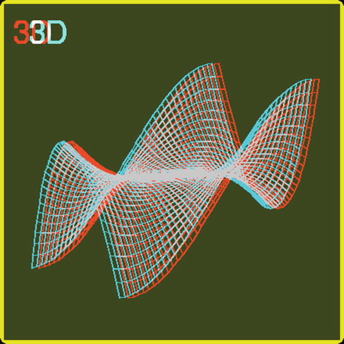
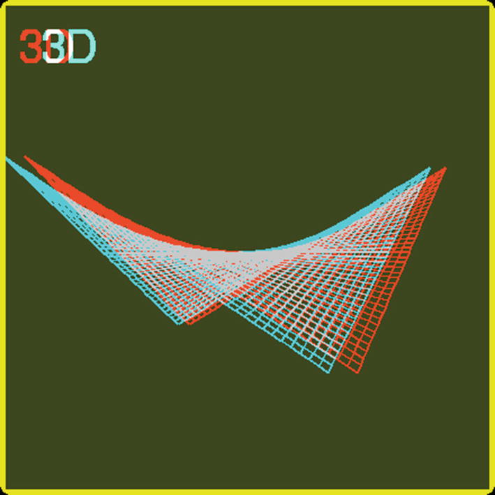
Plot obtained with the program of Equation (8.1) showing a saddle point

Another equation showing a typical saddle point is as follows:
$$ fleft(x,y
ight)= xy $$
(8.2)
The corresponding plot obtained with this program is shown in Figure 8-3.
../images/510726_1_En_8_Chapter/510726_1_En_8_Fig3_HTML.jpg
Figure 8-3

Plot obtained with the program of Equation (8.2) showing a saddle point

8.5 Summary

In this chapter, we described elements for constructing stereoscopic 3D plots of analytical functions. We showed how to incorporate the coordinates and the mesh. Additionally, we described how to create the required PIL images that are ORed and convert the resulting image into a Kivy one to display it on the screen.

..................Content has been hidden....................

You can't read the all page of ebook, please click here login for view all page.
Reset
3.14.6.194