© The Author(s), under exclusive license to APress Media, LLC, part of Springer Nature 2021
M. Cywiak, D. CywiakMulti-Platform Graphics Programming with Kivyhttps://doi.org/10.1007/978-1-4842-7113-1_16

16. Stereoscopic Plotting of Three-Dimensional Conics

Moisés Cywiak1   and David Cywiak2
(1)
Leon, Guanajuato, Mexico
(2)
Queretaro, Mexico
 
In this chapter, we describe basic principles for plotting stereoscopic three-dimensional conics. Figure 16-1 shows two screenshots of this program running on an Android cell phone showing plots of a hyperboloid at two different angles of rotation.
../images/510726_1_En_16_Chapter/510726_1_En_16_Fig1_HTML.jpg
Figures 16-1

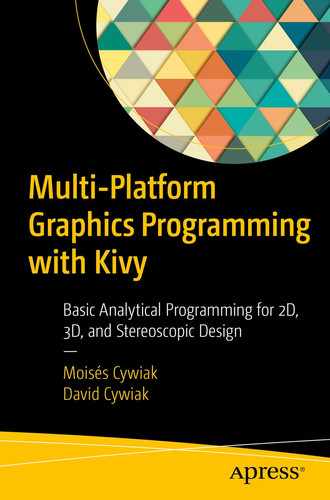
The program running on an Android cell phone showing plots of a hyperboloid at two different angles of rotation

The functionality of the buttons in the program is the same as in previous chapters.

In the following section, we describe the analytical approach.

16.1 Analytical Approach

Let’s consider an ellipse on the coordinate plane x-y, as depicted in Figure 16-2.
../images/510726_1_En_16_Chapter/510726_1_En_16_Fig2_HTML.jpg
Figure 16-2

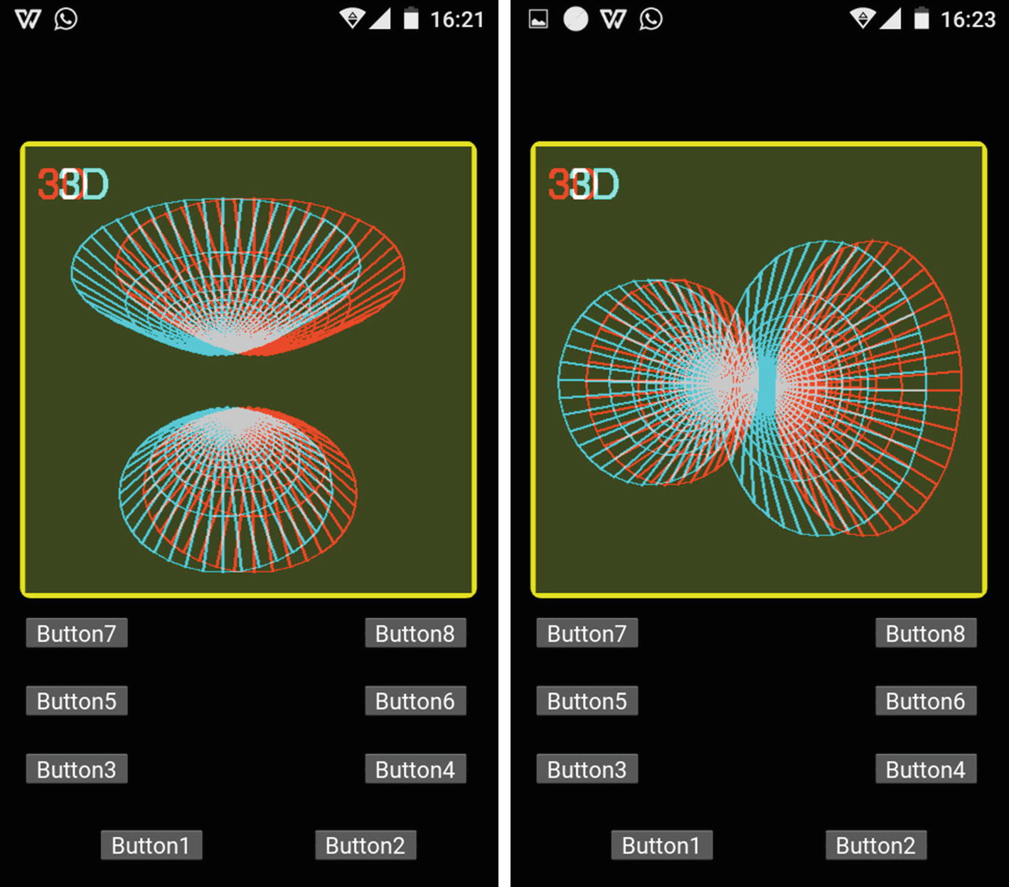
Ellipse on a coordinate plane x-y

The equation of the ellipse can be written as follows:
$$ frac{x2}{a^{{}^2}}+frac{y^{{}^2}}{b^{{}^2}}=1 $$
(16.1)

In Equation (16.1), as usual, the constant parameters a and b represent the length of the horizontal and vertical semi-axes, respectively.

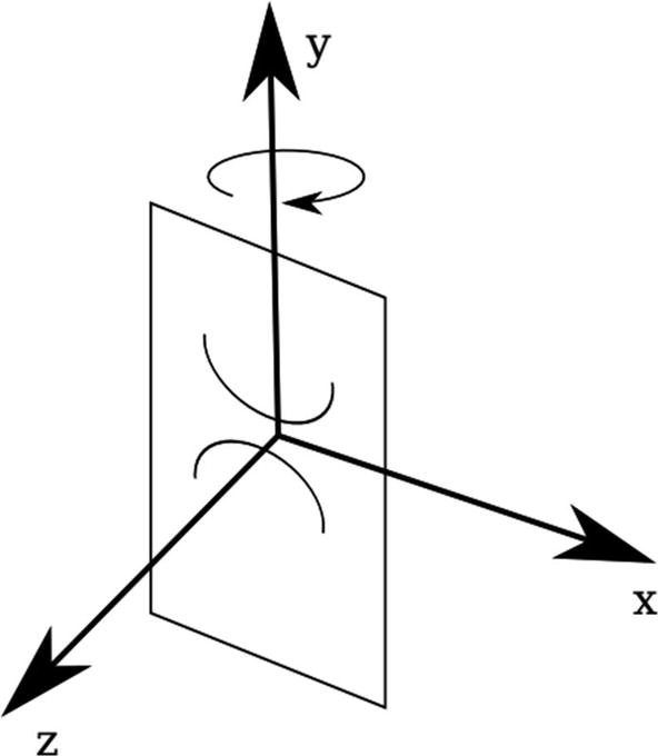
Let’s consider a point with coordinates (xP, yP) on the plane x-y, at an arbitrary position on the ellipse and pointed by a vector rp, as depicted in Figure 16-2.

The goal is to generate a three-dimensional ellipsoid by rotating the plane that contains the ellipse of Figure 16-2 around the y-axis, as depicted in Figure 16-3. The three-dimensional geometric plot, so generated, will be referred to as an ellipsoid of rotation. In this example, the ellipse rotates about one of its principal axes. Then, the plot so generated is known as an ellipsoid of revolution.
../images/510726_1_En_16_Chapter/510726_1_En_16_Fig3_HTML.jpg
Figure 16-3

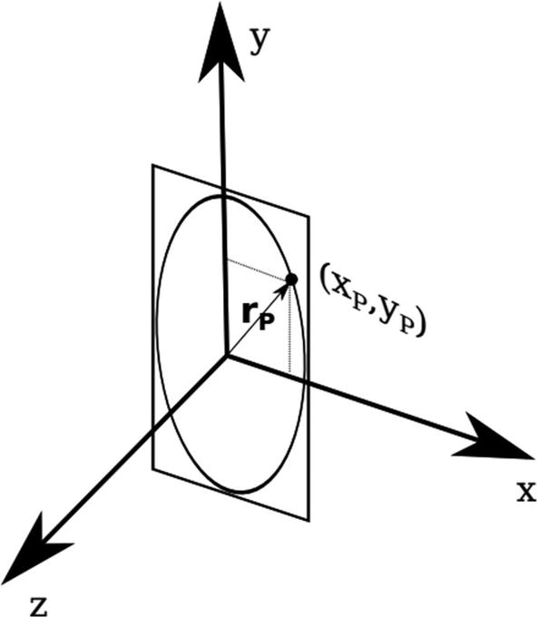
Rotation of the ellipse in Figure 16-2

In Figure 16-3, let r = xi + yj + zk and rp = xpi + ypj, where i, j, and k are the Cartesian unit direction vectors. Note that the magnitude of r and rp are equal. Therefore, we can write the following:
$$ {x}^{{}^2}+{y}^{{}^2}+{z}^{{}^2}={x_p}^{{}^2}+{y_p}^{{}^2} $$
(16.2)

Since the point (xP, yP) is a point of the ellipse, it satisfies Equation (16.1).

It can be observed from Figure 16-3 that y = yp. Therefore, canceling equal terms in Equation (16.2) and using Equation (16.1) gives the following:
$$ frac{x^{{}^2}}{a^{{}^2}}+frac{y^{{}^2}}{b^{{}^2}}+frac{z^{{}^2}}{a^{{}^2}}=1 $$
(16.3)

Equation (16.3) represents an ellipse of revolution.

If in Equation (16.3), we allow all the constants to be different, we obtain a more general expression, written as follows:
$$ frac{x^{{}^2}}{a^{{}^2}}+frac{y^{{}^2}}{b^{{}^2}}+frac{z^{{}^2}}{c^{{}^2}}=1 $$
(16.4)

Equation (16.4) is the equation of a three-dimensional ellipsoid.

In the following section, we describe our stereoscopic plotting approach of the ellipsoid.

16.2 Stereoscopic Ellipsoid Plotting

This approach consists of representing the ellipsoid in spherical coordinates. Before doing so, it is necessary to consider that in our geometrical situation, the vertical axis corresponds to y. The horizontal axis corresponds to x and z represents depth. Therefore, for programming purposes, we will rewrite Equation (16.4) as follows:
$$ frac{y^{{}^2}}{a^{{}^2}}+frac{x^{{}^2}}{b^{{}^2}}+frac{z^{{}^2}}{c^{{}^2}}=1 $$
(16.5)
Accordingly, the spherical system will be represented as in Figure 16-4.
../images/510726_1_En_16_Chapter/510726_1_En_16_Fig4_HTML.jpg
Figure 16-4

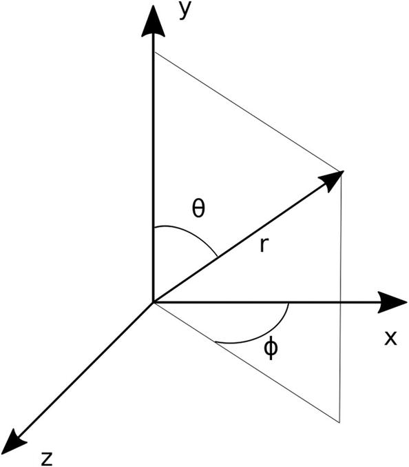
Spherical coordinate system used in this program

From Figure 16-4, the coordinates of the position vector can be written as follows:
$$ x= rsinleft(	heta 
ight)mathit{cos}left(phi 
ight) $$
(16.6)
$$ y= rcosleft(	heta 
ight) $$
(16.7)
$$ z= rsinleft(	heta 
ight)mathit{sin}left(phi 
ight) $$
(16.8)
Substituting Equations (16.6)-(16.8) into Equation (16.5) gives the following equation:
$$ {left(frac{rcosleft(	heta 
ight)}{a}
ight)}^2+{left(frac{rsinleft(	heta 
ight)mathit{cos}left(phi 
ight)}{b}
ight)}^2+{left(frac{rsinleft(	heta 
ight)mathit{sin}left(phi 
ight)}{c}
ight)}^2=1 $$
(16.9)
From Equation (16.9), the radial distance r is expressed as follows:
$$ r=frac{1}{sqrt{{left(frac{mathit{cos}left(	heta 
ight)}{a}
ight)}^2+{left(frac{mathit{sin}left(	heta 
ight)mathit{cos}left(phi 
ight)}{b}
ight)}^2+{left(frac{mathit{sin}left(	heta 
ight)mathit{sin}left(phi 
ight)}{c}
ight)}^2}} $$
(16.10)

Equation (16.10) will be used to generate our plot.

We will first set the number of pixels and the constant ellipse values a, b, and c, as follows:
a=100; b=90; c=60;
Next we set the variable D, which is the distance between the plane of projection and the screen, to 800. We also set coordinates of the left and right points of projection, as follows:
D=800;
VX1=100; VY1=100; VZ1=0;
VX2=140; VY2=100; VZ2=0;
We will use the percentage variable P with the value 0.5 to place the ellipsoid in the middle, between the screen and the plane of projection. We also set the number of pixels as follows:
D=600; #Distance from plane of projection to screen
P=0.5; #Place the function at z=D/2
N=40;  #Number of pixels to represent the function
ZG0=P*D; # z Offset to place the function
Next, we create and fill the arrays corresponding to r, Theta, and Phi, as shown in Listing 16-1.
import numpy as np
Pi=np.pi;
Theta=np.zeros(N+1);
Phi=np.zeros(N+1);
r=np.zeros( (N+1,N+1) );
for n in range(0,N+1):
    Theta[n]=n/N*Pi;
    Phi[n]=n/N*2*Pi;
for n in range(0,N+1):
    for m in range(0,N+1):
        r[n][m]=1/np.sqrt( (np.sin(Theta[n])
                            *np.cos(Phi[m])/a)**2 +
              (np.sin(Theta[n])*np.sin(Phi[m])/b)**2
                        +(np.cos(Theta[n])/c)**2  );
Listing 16-1

Creating and Filling the r, Theta, and Phi Arrays

In this code, Theta entries range from 0 to π, and Phi ranges from 0 to 2π. Both arrays have N+1 entries. The radial distance is represented by the two-dimensional array (N+1) x (N+1), r, and stores the values given by Equation (16.10).

The next step consists of creating and filling the mesh. The code is shown in Listing 16-2.
x1=np.zeros( (N+1,N+1) ); z1=np.zeros( (N+1,N+1) );
for n in range (0,N+1):
    for m in range(0,N+1):#Filling Mesh
        x1[n][m]=r[n][m]*np.sin(Theta[n])
                                  *np.cos(Phi[m]);
        z1[n][m]=r[n][m]*np.sin(Theta[n])
                              *np.sin(Phi[m])+ZG0;
        y[n][m]=r[n][m]*np.cos(Theta[n]);
Listing 16-2

Creating Mesh Arrays

The two nested for loops are used to fill the mesh according to Equations (16.6)-(16.8).

The functions to plot and rotate the ellipsoid are similar to their corresponding ones described in previous chapters. Figure 16-5 shows a stereoscopic plot of an ellipsoid with a=100, b=90, and c=60, obtained with the program code.
../images/510726_1_En_16_Chapter/510726_1_En_16_Fig5_HTML.jpg
Figure 16-5

Stereoscopic scene of an ellipsoid with a=100, b=90, and c=60, plotted with the code

The complete code listings for main.py and File.kv are shown in Listings 16-3 and 16-4, respectively.
from kivy.app import App
from kivy.uix.floatlayout import FloatLayout
from kivy.graphics import Line, Ellipse, Color
from kivy.clock import Clock
from kivy.core.image import Image as CoreImage
from PIL import Image, ImageDraw, ImageFont
import io
import os
import numpy as np
from kivy.lang import Builder
Builder.load_file(
    os.path.join(os.path.dirname(os.path.abspath(
                            __file__)), 'File.kv')
                  );
#Avoid Form1 of being resizable
from kivy.config import Config
Config.set("graphics","resizable", False);
Config.set('graphics', 'width',  '480');
Config.set('graphics', 'height', '680');
D=800;
VX1=100; VY1=100; VZ1=0;
VX2=140; VY2=100; VZ2=0;
P=0.5; #Place the function at z=D/2
N=40;  #Number of pixels to represent the function
y=np.zeros( (N+1,N+1) );
#creating Mesh arrays
x1=np.zeros( (N+1,N+1) ); z1=np.zeros( (N+1,N+1) );
L=130;  r0=L/5;
XG0=0; ZG0=P*D; Amplitude=150;
a=40; b=40; c=60;
Pi=np.pi;
Theta=np.zeros(N+1);
Phi=np.zeros(N+1);
r=np.zeros( (N+1,N+1) );
for n in range(0,N+1):
    Theta[n]=n/N*Pi;
    Phi[n]=n/N*2*Pi;
for n in range(0,N+1):
    for m in range(0,N+1):
        r[n][m]=1/np.sqrt( (np.sin(Theta[n])
                            *np.cos(Phi[m])/a)**2 +
              (np.sin(Theta[n])*np.sin(Phi[m])/b)**2
                        +(np.cos(Theta[n])/c)**2  );
for n in range (0,N+1):
    for m in range(0,N+1):#Filling Mesh
        x1[n][m]=r[n][m]*np.sin(Theta[n])
                                  *np.cos(Phi[m]);
        z1[n][m]=r[n][m]*np.sin(Theta[n])
                              *np.sin(Phi[m])+ZG0;
        y[n][m]=r[n][m]*np.cos(Theta[n]);
PointList=np.zeros( (N+1,2) );
def GraphFunction(VX,VY,VZ,Which):
    global x1,y, z1, N;
    #MaxY=np.max(y)
    if (Which==0):
        r,g,b = 200, 0, 0; #red Image
        Draw=Draw1
    else:
        r,g,b= 0, 200, 200; #cyan image
        Draw=Draw2
    for n in range (0,N+1): #Horizontal Lines
        for m in range (0,N+1):
            Factor=(D-VZ)/(D-z1[n][m]-VZ);
            xA=XC+Factor*(x1[n][m]-VX)+VX;
            yA=YC-Factor*(y[n][m]-VY)-VY;
            PointList[m]=xA,yA;
        List=tuple( map(tuple,PointList) );
        Draw.line( List, fill=(r,g,b), width=2 );
    for n in range (0,N+1): #Vertical Lines
        for m in range (0,N+1):
            Factor=(D-VZ)/(D-z1[m][n]-VZ);
            xA=XC+Factor*(x1[m][n]-VX)+VX;
            yA=YC-Factor*(y[m][n]-VY)-VY;
            PointList[m]=xA,yA;
        List=tuple( map(tuple,PointList) );
        Draw.line( List, fill=(r,g,b), width=2 );
        Font = ImageFont.truetype('Gargi.ttf', 40)
        Draw1.text( (10,10), "3D", fill =
                            (255,0,0,1), font=Font);
        Draw2.text( (30,10), "3D", fill =
                          (0,255,255,1), font=Font);
def ShowScene(B):
    Array1=np.array(PilImage1);
    Array2=np.array(PilImage2);
    Array3=Array1 | Array2;
    PilImage3=Image.fromarray(Array3);
    Memory=io.BytesIO();
    PilImage3.save(Memory, format="png");
    Memory.seek(0);
    ImagePNG=CoreImage(Memory, ext="png");
    B.ids.Screen1.texture=ImagePNG.texture;
    ImagePNG.remove_from_cache()
    Memory.close();
    PilImage3.close();
    Array1=None;
    Array2=None;
    Array3=None;
def ClearObjects():
    Draw1.rectangle( (0, 0, W-10, H-10), fill =
                                 (60, 70, 30, 1) );
    Draw2.rectangle( (0, 0, W-10, H-10), fill =
                                 (60, 70, 30, 1) );
def RotateFunction(B, Sense):
    global XG0, ZG0
    if Sense==-1:
        Teta=np.pi/180*(-4.0);
    else:
        Teta=np.pi/180*(4.0);
    Cos_Teta=np.cos(Teta)
    Sin_Teta=np.sin(Teta);
    X0=XG0;  Y0=0;  Z0=ZG0 # Center of rotation
    for n in range(0,N+1):
        for m in range(0,N+1):
            if (B.ids.Button3.state=="down" or
                       B.ids.Button4.state=="down"):
                yP=(y[n][m]-Y0)*Cos_Teta
                    + (x1[n][m]-X0)*Sin_Teta + Y0;
                xP=-(y[n][m]-Y0)*Sin_Teta
                        +(x1[n][m]-X0)*Cos_Teta + X0;
                y[n][m]=yP;
                x1[n][m]=xP;
            if (B.ids.Button5.state=="down" or
                       B.ids.Button6.state=="down"):
                yP=(y[n][m]-Y0)*Cos_Teta
                      + (z1[n][m]-Z0)*Sin_Teta + Y0;
                zP=-(y[n][m]-Y0)*Sin_Teta
                      + (z1[n][m]-Z0)*Cos_Teta + Z0;
                y[n][m]=yP;
                z1[n][m]=zP;
            if (B.ids.Button7.state=="down" or
                       B.ids.Button8.state=="down"):
                xP=(x1[n][m]-X0)*Cos_Teta
                      + (z1[n][m]-Z0)*Sin_Teta + X0;
                zP=-(x1[n][m]-X0)*Sin_Teta
                       +(z1[n][m]-Z0)*Cos_Teta + Z0;
                x1[n][m]=xP;
                z1[n][m]=zP;
class Form1(FloatLayout):
    def __init__(Handle, **kwargs):
        super(Form1, Handle).__init__(**kwargs);
        Event1=Clock.schedule_once(Handle.Initialize);
    def Initialize(B, *args):
        global W,H, XC,YC;
        global PilImage1,PilImage2, Draw1,Draw2;
        # P= Percentage of the D distance
        global P, Amplitude;
        W,H=B.ids.Screen1.size;
        XC=int (W/2)+P/(1-P)*VX1+18;
        YC=int(H/2)-P/(1-P)*VY1+10;
        PilImage1= Image.new('RGB', (W-10, H-10),
                                     (60, 70, 30));
        Draw1 = ImageDraw.Draw(PilImage1);
        PilImage2= Image.new('RGB', (W-10, H-10),
                                     (60, 70, 30));
        Draw2 = ImageDraw.Draw(PilImage2);
        Font = ImageFont.truetype('Gargi.ttf', 70)
        Draw1.text( (30,200), "3D Images", fill =
                            (255,0,0,1), font=Font);
        Draw2.text( (50,200), "3D Images", fill =
                          (0,255,255,1), font=Font);
        ShowScene(B);
    def Button1_Click(B):
        global Draw1, Draw2;
        ClearObjects(); # Clearing Draw1 and Draw2
        GraphFunction(VX1,VY1,VZ1,0);
        GraphFunction(VX2,VY2,VZ2,1);
        ShowScene(B);
    def Button2_Click(B):
        ClearObjects(); # Clearing Draw1 and Draw2
        Font = ImageFont.truetype('Gargi.ttf', 70)
        Draw1.text( (30,200), "3D Images", fill =
                            (255,0,0,1), font=Font);
        Draw2.text( (50,200), "3D Images", fill =
                          (0,255,255,1), font=Font);
        ShowScene(B);
    def Button3_Click(B):
        RotateFunction(B,1);
        ClearObjects(); # Clearing Draw1 and Draw2
        GraphFunction(VX1,VY1,VZ1,0);
        GraphFunction(VX2,VY2,VZ2,1);
        ShowScene(B);
    def Button4_Click(B):
        RotateFunction(B,-1),
        ClearObjects();
        GraphFunction(VX1,VY1,VZ1,0);
        GraphFunction(VX2,VY2,VZ2,1);
        ShowScene(B);
    def Button5_Click(B):
        RotateFunction(B,-1),
        ClearObjects();
        GraphFunction(VX1,VY1,VZ1,0);
        GraphFunction(VX2,VY2,VZ2,1);
        ShowScene(B);
    def Button6_Click(B):
        RotateFunction(B,1),
        ClearObjects();
        GraphFunction(VX1,VY1,VZ1,0);
        GraphFunction(VX2,VY2,VZ2,1);
        ShowScene(B);
    def Button7_Click(B):
        RotateFunction(B,-1),
        ClearObjects();
        GraphFunction(VX1,VY1,VZ1,0);
        GraphFunction(VX2,VY2,VZ2,1);
        ShowScene(B);
    def Button8_Click(B):
        RotateFunction(B,1),
        ClearObjects();
        GraphFunction(VX1,VY1,VZ1,0);
        GraphFunction(VX2,VY2,VZ2,1);
        ShowScene(B);
# This is the Start Up code.
class StartUp (App):
    def build (BU):
        BU.title="Form1"
        return Form1();
if __name__ =="__main__":
    StartUp().run();
Listing 16-3

Code for the main.py (Ellipsoid) File

#:set W 440
#:set H 440
<Form1>:
    id : Form1
    Image:
        id: Screen1
        size_hint: None,None
        pos_hint: {"x":0.04, "y":0.34}
        size: W,H
        canvas.before:
            Color:
                rgba: 0.9, 0.9, 0, 1
            RoundedRectangle:
                pos:  self.pos
                size: self.size
    Button:
        id: Button1
        on_press: Form1.Button1_Click()
        text: "Button1"
        size_hint: None,None
        pos_hint: {"x": 0.2, "y":0.03}
        size: 100,30
    Button:
        id: Button2
        on_press: Form1.Button2_Click()
        text: "Button2"
        size_hint: None,None
        pos_hint: {"x": 0.63, "y":0.03}
        size: 100,30
    Button:
        id: Button3
        on_press: Form1.Button3_Click()
        text: "Button3"
        size_hint: None,None
        pos_hint: {"x": 0.05, "y":0.12}
        size: 100,30
        always_release: True
    Button:
        id: Button4
        on_press: Form1.Button4_Click()
        text: "Button4"
        size_hint: None,None
        pos_hint: {"x": 0.73, "y":0.12}
        size: 100,30
    Button:
        id: Button5
        on_press: Form1.Button5_Click()
        text: "Button5"
        size_hint: None,None
        pos_hint: {"x": 0.05, "y":0.20}
        size: 100,30
    Button:
        id: Button6
        on_press: Form1.Button6_Click()
        text: "Button6"
        size_hint: None,None
        pos_hint: {"x": 0.73, "y":0.20}
        size: 100,30
    Button:
        id: Button7
        on_press: Form1.Button7_Click()
        text: "Button7"
        size_hint: None,None
        pos_hint: {"x": 0.05, "y":0.28}
        size: 100,30
    Button:
        id: Button8
        on_press: Form1.Button8_Click()
        text: "Button8"
        size_hint: None,None
        pos_hint: {"x": 0.73, "y":0.28}
        size: 100,30
Listing 16-4

Code for the file.kv File

16.3 Hyperboloid

As in the case of the ellipsoid, we will first consider the equation of a hyperbola on the x-y plane.

For programming purposes and without loss of generality, we focus on a vertical hyperbola, as depicted in Figure 16-6.
../images/510726_1_En_16_Chapter/510726_1_En_16_Fig6_HTML.jpg
Figure 16-6

Vertical hyperbola on the plane x-y

The equation for the vertical hyperbola can be written as follows:
$$ frac{x^{{}^2}}{a^{{}^2}}-frac{y^{{}^2}}{b^{{}^2}}=1 $$
(16.11)
We now allow the plane of the hyperbola to rotate in a similar manner as we did with the ellipse. Then, using Equation (16.11) and Equation (16.2), we obtain the equation of a vertical circular hyperboloid as follows:
$$ frac{x^{{}^2}}{a^{{}^2}}-frac{y^{{}^2}}{b^{{}^2}}-frac{z^{{}^2}}{b^{{}^2}}=1 $$
(16.12)
By allowing the constant terms that correspond to x, y, and z to be different between them in Equation (16.12), we’ll create a more general vertical hyperboloid equation. Using our geometrical situation, the equation is as follows:
$$ frac{y^{{}^2}}{a^{{}^2}}-frac{x^{{}^2}}{b^{{}^2}}-frac{z^{{}^2}}{c^{{}^2}}=1 $$
(16.13)
To plot the hyperboloid given by Equation (16.13), we use spherical coordinates in a similar way as we did with the ellipsoid in Section 16.2. Then, substituting Equations (16.6)-(16.8) into Equation (16.13) gives the following:
$$ {left(frac{rcosleft(	heta 
ight)}{a}
ight)}^2-{left(frac{rsinleft(	heta 
ight)mathit{cos}left(phi 
ight)}{b}
ight)}^2-{left(frac{rsinleft(	heta 
ight)mathit{sin}left(phi 
ight)}{c}
ight)}^2=1 $$
(16.14)
Using Equation (16.14) gives the following:
$$ r=frac{1}{sqrt{{left(frac{mathit{cos}left(	heta 
ight)}{a}
ight)}^2-{left(frac{mathit{sin}left(	heta 
ight)mathit{cos}left(phi 
ight)}{b}
ight)}^2-{left(frac{mathit{sin}left(	heta 
ight)mathit{sin}left(phi 
ight)}{c}
ight)}^2}} $$
(16.15)

The argument within the square root in Equation (16.15) can be zero or negative for some values. Therefore, the radial distance can result in an undefined or a complex number. This characteristic is a natural consequence of the hyperboloid shape, as it consists of two separated surfaces. Therefore, to avoid plotting at these values, we will proceed as follows.

We will vary the angle ϕ between 0 and 2π. However, the values that θ can take must be split into two intervals, one for plotting the upper surface and the other for the bottom surface. The first interval is between 0 and some value θ0< θMax and the second one is between π and π + θ0. Here, θMax is the maximum allowed value that θ can take to avoid undefined or complex values in Equation (16.15). It is possible to exactly calculate θMax; however, for illustrative purposes, it will be sufficient to propose and test some values.

Because the θ variable requires two angular intervals, it will be convenient to use two independent arrays, which we call ThetaA and ThetaB. For the variable ϕ, only one array is required, called Phi. The code for creating and filling the arrays is shown in Listing 16-5.
import numpy as np
N=40; Pi=np.pi;
Theta0=Pi/180*(40);
Phi=np.zeros(N+1);
ThetaA=np.zeros(N+1); rA=np.zeros( (N+1,N+1) );
ThetaB=np.zeros(N+1); rB=np.zeros( (N+1,N+1) );
for n in range(0,N+1):
    ThetaA[n]=n/N*Theta0; #from 0 to Theta0
    ThetaB[n]=n/N*Theta0 +Pi; #from Pi to(Pi+Theta0)
Phi0=Pi/180*360
for n in range(0,N+1):
    Phi[n]=(n-N/2)/N*Phi0;
Listing 16-5

Filling Two Independent Arrays for the Hyperboloid

In this code, θ0, represented in the code by Theta0, was set to 40 degrees. We set this value arbitrarily as a first trial. The multiplying factor π/180 converts entries from degrees to radians. For simplicity, we tested different values for θ0, taking care of attaining only real values for the radial distance as given by Equation (16.15). The ThetaA, ThetaB, and Phi arrays all have sizes N+1.

Next, since we will plot the upper and bottom surfaces independently, we need to create two mesh sets, as shown in Listing 16-6.
y1A=np.zeros( (N+1,N+1) );
y1B=np.zeros( (N+1,N+1) );
x1A=np.zeros( (N+1,N+1) );
x1B=np.zeros( (N+1,N+1) );
z1A=np.zeros( (N+1,N+1) ); #Mesh
z1B=np.zeros( (N+1,N+1) ); #Mesh
Listing 16-6

Creating Two Mesh Sets

For the two surfaces, we need two arrays for the radial distance. Each array will be filled with values given by Equation (16.14). The corresponding code is shown in Listing 16-7.
rA=np.zeros( (N+1,N+1) );  rB=np.zeros( (N+1,N+1) );
for n in range(0,N+1):
    for m in range(0,N+1):
        rA[n][m]=1/np.sqrt( (np.cos(ThetaA[n])/a)**2
            -(np.sin(ThetaA[n])*np.sin(Phi[m])/b)**2
        -(np.sin(ThetaA[n])*np.cos(Phi[m])/c)**2  );
        rB[n][m]=1/np.sqrt( (np.cos(ThetaB[n])/a)**2
            -(np.sin(ThetaB[n])*np.sin(Phi[m])/b)**2
         -(np.sin(ThetaB[n])*np.cos(Phi[m])/c)**2  );
Listing 16-7

Creating Two Arrays for the Radial Distances

We can fill both mesh values using Equations (16.6)-(16.8), as shown in Listing 16-8.
L=5;
for n in range (0,N+1):
    for m in range(0,N+1):#Filling MeshA
        x1A[n][m]=L*rA[n][m]*np.sin(ThetaA[n])*
                                   np.cos(Phi[m]);
        z1A[n][m]=L*rA[n][m]*np.sin(ThetaA[n])*
                               np.sin(Phi[m])+ZG0;
        y1A[n][m]=L*rA[n][m]*np.cos(ThetaA[n]);
for n in range (0,N+1):
    for m in range(0,N+1):#Filling MeshB
        x1B[n][m]=L*rB[n][m]*np.sin(ThetaB[n])
                                   *np.cos(Phi[m]);
        z1B[n][m]=L*rB[n][m]*np.sin(ThetaB[n])
                               *np.sin(Phi[m])+ZG0;
        y1B[n][m]=L*rB[n][m]*np.cos(ThetaB[n]);
Listing 16-8

Filling the Two Mesh Values

In this code listing, L is a scaling factor that allows us to change the dimensions of the plot.

The GraphFunction (VX,VY,VZ,Which) and RotateFunction (B, Sense) functions are similar to the ones described in previous chapters. There is a slight difference, however. Instead of using one array for plotting only one surface, these functions use two arrays for plotting the upper and bottom surfaces.

The code for main.py that corresponds to the hyperboloid is shown in Listing 16-9.
from kivy.app import App
from kivy.uix.floatlayout import FloatLayout
from kivy.graphics import Line, Ellipse, Color
from kivy.clock import Clock
from kivy.core.image import Image as CoreImage
from PIL import Image, ImageDraw, ImageFont
import io
import os
import numpy as np
from kivy.lang import Builder
Builder.load_file(
    os.path.join(os.path.dirname(os.path.abspath(
                            __file__)), 'File.kv')
                  );
#Avoid Form1 of being resizable
from kivy.config import Config
Config.set("graphics","resizable", False);
Config.set('graphics', 'width',  '480');
Config.set('graphics', 'height', '680');
D=600;
VX1=-15; VY1=0; VZ1=0;
VX2=15; VY2=0; VZ2=0;
P=0.0; #Place the function at z=D/2
N=40;  #Number of pixels to represent the function
y1A=np.zeros( (N+1,N+1) );
y1B=np.zeros( (N+1,N+1) );
x1A=np.zeros( (N+1,N+1) );
x1B=np.zeros( (N+1,N+1) );
z1A=np.zeros( (N+1,N+1) ); #Mesh
z1B=np.zeros( (N+1,N+1) ); #Mesh
XG0=0; ZG0=P*D;
a=10; b=9; c=9;
Pi=np.pi;
Theta0=Pi/180*(40);
Phi=np.zeros(N+1);
ThetaA=np.zeros(N+1); rA=np.zeros( (N+1,N+1) );
ThetaB=np.zeros(N+1); rB=np.zeros( (N+1,N+1) );
for n in range(0,N+1):
    ThetaA[n]=n/N*Theta0; #from 0 to Theta0
    ThetaB[n]=n/N*Theta0 +Pi; #from Pi to(Pi+Theta0)
Phi0=Pi/180*360
for n in range(0,N+1):
    Phi[n]=(n-N/2)/N*Phi0;
for n in range(0,N+1):
    for m in range(0,N+1):
        rA[n][m]=1/np.sqrt( (np.cos(ThetaA[n])/a)**2
            -(np.sin(ThetaA[n])*np.sin(Phi[m])/b)**2
        -(np.sin(ThetaA[n])*np.cos(Phi[m])/c)**2  );
        rB[n][m]=1/np.sqrt( (np.cos(ThetaB[n])/a)**2
            -(np.sin(ThetaB[n])*np.sin(Phi[m])/b)**2
         -(np.sin(ThetaB[n])*np.cos(Phi[m])/c)**2  );
L=5;
for n in range (0,N+1):
    for m in range(0,N+1):#Filling MeshA
        x1A[n][m]=L*rA[n][m]*np.sin(ThetaA[n])*
                                   np.cos(Phi[m]);
        z1A[n][m]=L*rA[n][m]*np.sin(ThetaA[n])*
                               np.sin(Phi[m])+ZG0;
        y1A[n][m]=L*rA[n][m]*np.cos(ThetaA[n]);
for n in range (0,N+1):
    for m in range(0,N+1):#Filling MeshB
        x1B[n][m]=L*rB[n][m]*np.sin(ThetaB[n])
                                   *np.cos(Phi[m]);
        z1B[n][m]=L*rB[n][m]*np.sin(ThetaB[n])
                               *np.sin(Phi[m])+ZG0;
        y1B[n][m]=L*rB[n][m]*np.cos(ThetaB[n]);
PointList=np.zeros( (N+1,2) );
def GraphFunction(VX,VY,VZ,Which):
    if (Which==0):
        r,g,b = 200, 0, 0; #red Image
        Draw=Draw1
    else:
        r,g,b= 0, 200, 200; #cyan image
        Draw=Draw2
    #Drawing surface A
    for n in range (0,N+1): #Horizontal Lines A
        for m in range (0,N+1):
            Factor=(D-VZ)/(D-z1A[n][m]-VZ);
            xA=XC+Factor*(x1A[n][m]-VX)+VX;
            yA=YC-Factor*(y1A[n][m]-VY)-VY;
            PointList[m]=xA,yA;
        List=tuple( map(tuple,PointList) );
        Draw.line( List, fill=(r,g,b), width=2 );
    for n in range (0,N+1): #Vertical Lines A
        for m in range (0,N+1):
            Factor=(D-VZ)/(D-z1A[m][n]-VZ);
            xA=XC+Factor*(x1A[m][n]-VX)+VX;
            yA=YC-Factor*(y1A[m][n]-VY)-VY;
            PointList[m]=xA,yA;
        List=tuple( map(tuple,PointList) );
        Draw.line( List, fill=(r,g,b), width=2 );
    #Drawing surface B
    for n in range (0,N+1): #Horizontal Lines B
        for m in range (0,N+1):
            Factor=(D-VZ)/(D-z1B[n][m]-VZ);
            xA=XC+Factor*(x1B[n][m]-VX)+VX;
            yA=YC-Factor*(y1B[n][m]-VY)-VY;
            PointList[m]=xA,yA;
        List=tuple( map(tuple,PointList) );
        Draw.line( List, fill=(r,g,b), width=2 );
    for n in range (0,N+1): #Vertical Lines B
        for m in range (0,N+1):
            Factor=(D-VZ)/(D-z1B[m][n]-VZ);
            xA=XC+Factor*(x1B[m][n]-VX)+VX;
            yA=YC-Factor*(y1B[m][n]-VY)-VY;
            PointList[m]=xA,yA;
        List=tuple( map(tuple,PointList) );
        Draw.line( List, fill=(r,g,b), width=2 );
        Font = ImageFont.truetype('Gargi.ttf', 40);
        Draw1.text( (10,10), "3D", fill =
                        (255,0,0,1),font=Font);
        Draw2.text( (30,10), "3D", fill =
                        (0,255,255,1), font=Font);
def ShowScene(B):
    Array1=np.array(PilImage1);
    Array2=np.array(PilImage2);
    Array3=Array1 | Array2;
    PilImage3=Image.fromarray(Array3);
    Memory=io.BytesIO();
    PilImage3.save(Memory, format="png");
    Memory.seek(0);
    ImagePNG=CoreImage(Memory, ext="png");
    B.ids.Screen1.texture=ImagePNG.texture;
    ImagePNG.remove_from_cache()
    Memory.close();
    PilImage3.close();
    Array1=None;
    Array2=None;
    Array3=None;
def ClearObjects():
    Draw1.rectangle( (0, 0, W-10, H-10), fill=
                             (60, 70, 30, 1) );
    Draw2.rectangle( (0, 0, W-10, H-10), fill=
                             (60, 70, 30, 1) );
def RotateFunction(B, Sense):
    global XG0, ZG0
    if Sense==-1:
        Teta=np.pi/180*(-4.0);
    else:
        Teta=np.pi/180*(4.0);
    Cos_Teta=np.cos(Teta)
    Sin_Teta=np.sin(Teta);
    X0=XG0;  Y0=0;  Z0=ZG0 # Center of rotation
    for n in range(0,N+1):
        for m in range(0,N+1):
            if (B.ids.Button3.state=="down" or
                    B.ids.Button4.state=="down"):
                yP=(y1A[n][m]-Y0)*Cos_Teta
                    + (x1A[n][m]-X0)*Sin_Teta + Y0;
                xP=-(y1A[n][m]-Y0)*Sin_Teta
                    +(x1A[n][m]-X0)*Cos_Teta + X0;
                y1A[n][m]=yP;
                x1A[n][m]=xP;
                yP=(y1B[n][m]-Y0)*Cos_Teta
                    + (x1B[n][m]-X0)*Sin_Teta + Y0;
                xP=-(y1B[n][m]-Y0)*Sin_Teta
                     +(x1B[n][m]-X0)*Cos_Teta + X0;
                y1B[n][m]=yP;
                x1B[n][m]=xP;
            if (B.ids.Button5.state=="down" or
                       B.ids.Button6.state=="down"):
                yP=(y1A[n][m]-Y0)*Cos_Teta
                    + (z1A[n][m]-Z0)*Sin_Teta + Y0;
                zP=-(y1A[n][m]-Y0)*Sin_Teta
                     +(z1A[n][m]-Z0)*Cos_Teta + Z0;
                y1A[n][m]=yP;
                z1A[n][m]=zP;
                yP=(y1B[n][m]-Y0)*Cos_Teta
                    + (z1B[n][m]-Z0)*Sin_Teta + Y0;
                zP=-(y1B[n][m]-Y0)*Sin_Teta
                     +(z1B[n][m]-Z0)*Cos_Teta + Z0;
                y1B[n][m]=yP;
                z1B[n][m]=zP;
            if (B.ids.Button7.state=="down" or
                       B.ids.Button8.state=="down"):
                xP=(x1A[n][m]-X0)*Cos_Teta
                    + (z1A[n][m]-Z0)*Sin_Teta + X0;
                zP=-(x1A[n][m]-X0)*Sin_Teta
                     +(z1A[n][m]-Z0)*Cos_Teta + Z0;
                x1A[n][m]=xP;
                z1A[n][m]=zP;
                xP=(x1B[n][m]-X0)*Cos_Teta
                    + (z1B[n][m]-Z0)*Sin_Teta + X0;
                zP=-(x1B[n][m]-X0)*Sin_Teta
                     +(z1B[n][m]-Z0)*Cos_Teta + Z0;
                x1B[n][m]=xP;
                z1B[n][m]=zP;
class Form1(FloatLayout):
    def __init__(Handle, **kwargs):
        super(Form1, Handle).__init__(**kwargs);
        Event1=Clock.schedule_once(Handle.Initialize);
    def Initialize(B, *args):
        global W,H, XC,YC;
        global PilImage1,PilImage2, Draw1,Draw2;
        # P= Percentage of the D distance
        global P, Amplitude;
        W,H=B.ids.Screen1.size;
        XC=int (W/2)+P/(1-P)*VX1+0;
        YC=int(H/2)-P/(1-P)*VY1+10;
        PilImage1= Image.new('RGB', (W-10, H-10),
                                     (60, 70, 30));
        Draw1 = ImageDraw.Draw(PilImage1);
        PilImage2= Image.new('RGB', (W-10, H-10),
                                     (60, 70, 30));
        Draw2 = ImageDraw.Draw(PilImage2);
        Font = ImageFont.truetype('Gargi.ttf', 70)
        Draw1.text( (30,200), "3D Images", fill =
                            (255,0,0,1), font=Font);
        Draw2.text( (50,200), "3D Images", fill =
                          (0,255,255,1), font=Font);
        ShowScene(B);
    def Button1_Click(B):
        global Draw1, Draw2;
        ClearObjects(); # Clearing Draw1 and Draw2
        GraphFunction(VX1,VY1,VZ1,0);
        GraphFunction(VX2,VY2,VZ2,1);
        ShowScene(B);
    def Button2_Click(B):
        ClearObjects(); # Clearing Draw1 and Draw2
        Font = ImageFont.truetype('Gargi.ttf', 70)
        Draw1.text( (30,200), "3D Images", fill =
                            (255,0,0,1), font=Font);
        Draw2.text( (50,200), "3D Images", fill =
                          (0,255,255,1), font=Font);
        ShowScene(B);
    def Button3_Click(B):
        RotateFunction(B,1);
        ClearObjects(); # Clearing Draw1 and Draw2
        GraphFunction(VX1,VY1,VZ1,0);
        GraphFunction(VX2,VY2,VZ2,1);
        ShowScene(B);
    def Button4_Click(B):
        RotateFunction(B,-1),
        ClearObjects();
        GraphFunction(VX1,VY1,VZ1,0);
        GraphFunction(VX2,VY2,VZ2,1);
        ShowScene(B);
    def Button5_Click(B):
        RotateFunction(B,-1),
        ClearObjects();
        GraphFunction(VX1,VY1,VZ1,0);
        GraphFunction(VX2,VY2,VZ2,1);
        ShowScene(B);
    def Button6_Click(B):
        RotateFunction(B,1),
        ClearObjects();
        GraphFunction(VX1,VY1,VZ1,0);
        GraphFunction(VX2,VY2,VZ2,1);
        ShowScene(B);
    def Button7_Click(B):
        RotateFunction(B,-1),
        ClearObjects();
        GraphFunction(VX1,VY1,VZ1,0);
        GraphFunction(VX2,VY2,VZ2,1);
        ShowScene(B);
    def Button8_Click(B):
        RotateFunction(B,1),
        ClearObjects();
        GraphFunction(VX1,VY1,VZ1,0);
        GraphFunction(VX2,VY2,VZ2,1);
        ShowScene(B);
# This is the Start Up code.
class StartUp (App):
    def build (BU):
        BU.title="Form1"
        return Form1();
if __name__ =="__main__":
    StartUp().run();
Listing 16-9

main.py (for the Hyperboloid)

16.4 Summary

In this chapter, we introduced elements for plotting stereoscopic three-dimensional conics. We presented an analytical approach to constructing them. We also utilized working examples to illustrate the programming process.

..................Content has been hidden....................

You can't read the all page of ebook, please click here login for view all page.
Reset
3.142.197.198