
Screenshots from an Android cell phone showing a two-dimensional spatial-function (left) and its corresponding Fourier transform obtained with this program (right)
The functionality of Button1 to Button8 is the same as described in Chapter 5.
In this application, Button9 toggles the numerical indicator between 0 and 1. Accordingly, the screen shows the spatial function or its corresponding two-dimensional Fourier transform.
17.1 One-Dimensional Fourier Transform
Briefly speaking, the Fourier transform consists of an integral that transforms a function defined in an initial domain into another function in the frequency domain. The initial domain can be any n-dimensional space of interest.
The Fourier transform is frequently used in digital processing, probability, optics, quantum mechanics, economics, and many other fields. The transform can be one-, two-, three-, or n-dimensional.

In Equation (17.1), the function in the initial domain is f(x), and the transformed function in the frequency domain is F(u). The parameter i represents the imaginary unit. The initial domain is represented by the spatial x-coordinate and the frequency coordinate is represented by u.


A physical interpretation of Equation (17.5) consists of visualizing f(x) in Equation (17.2) as a vibrating string placed along the horizontal x-coordinate. The string vibrates vertically with a period equal to T, or equivalently with a frequency  . Then, Equation (17.5) indicates that the Fourier transform, F(u), consists of two well defined points in the frequency domain located at
  and
and  . We conclude, therefore, that when a string vibrates at a determined frequency, the Fourier transform consists of two points. The first one corresponds to the vibration frequency. The second, to the negative value of this frequency.

![$$ F(u)=left[frac{A_1}{2}delta left(u-frac{1}{T_1}
ight)+frac{A_1}{2}delta left(u+frac{1}{T_1}
ight)
ight]+left[frac{A_2}{2}delta left(u-frac{1}{T_2}
ight)+frac{A_1}{2}delta left(u+frac{1}{T_2}
ight)
ight] $$](https://imgdetail.ebookreading.net/202109/3/9781484271131/9781484271131__9781484271131__files__images__510726_1_En_17_Chapter__510726_1_En_17_Chapter_TeX_Equ7.png)
From Equation (17.7), we notice that the Fourier transform consists of two well-defined points for each vibrating frequency . Each point corresponds to the positive or negative value of a frequency. Each point in the frequency space has an amplitude equal to half of its corresponding one.
Considering that the string vibrates at multiple frequencies, each frequency with a corresponding amplitude, the Fourier transform will give points at all the frequencies of vibration, including positives and negatives, along with their corresponding half amplitude values. Therefore, the Fourier transform provides the amplitude distribution of frequencies of a vibrating object and its spectral distribution.
In the following section, we introduce two functions frequently encountered in Fourier analysis.
17.2 The Rectangular and Sinc Functions
Two functions of special interest in Fourier studies are the Rect(x, A) (rectangular) and the sinc(x) functions.

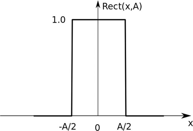
The Rect(x, A) Function


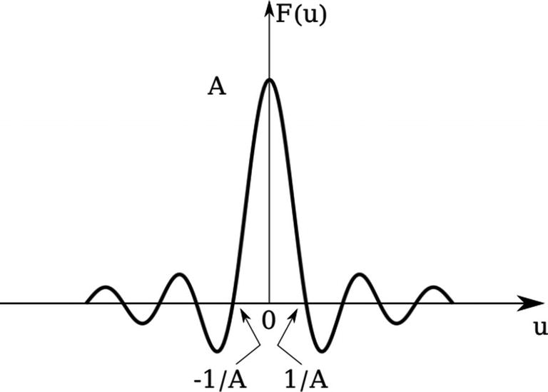
Plot of Asinc(Au). Intercepts with the u-axis occur at 
Although we want to focus on the two-dimensional Fourier transform, for illustrative purposes, we provide a brief code description for calculating the discrete one-dimensional Fourier transform in the next section.
17.3 Code for Calculating the Discrete One-Dimensional Fourier Transform
The Rect Function
To better represent this function in the one-dimensional case, we can use a large number of pixels while keeping a short processing time. This is in contrast to the two-dimensional case, where a small N increment can result in very high processing times.
The width of the rectangle function was set to L/(2.4).
Setting Values for x and f
In this for loop, we have assigned N+1 entries with values ranging from -L/2 to L/2 to the first array for storing the x-points. The N+1 values corresponding to the function are stored in the second array, f.
Setting Frequency Values
In the for loop, the frequency (or spectral) array, u, stores N+1 equally spaced values ranging from -B/2 to B/2. The value 10/A assigned to the parameter B is set based in our experience when calculating the sinc function depicted in Figure 17-3.
We have declared F as a one-dimensional array for storing N+1 complex numbers. This is necessary, as the calculations of the integral given by Equation (17.1) will give, in general, complex numbers.
At this point, u represents N+1 frequency points ranging from -B/2 to B/2. As a consequence, F(u) will be also represented by a discrete array, F.
![$$ Fleft[n
ight]={sum}_{m=0}^Nfleft[m
ight] mathit{exp}left(-i2pi uleft[n
ight]xleft[m
ight]
ight) dx $$](https://imgdetail.ebookreading.net/202109/3/9781484271131/9781484271131__9781484271131__files__images__510726_1_En_17_Chapter__510726_1_En_17_Chapter_TeX_Equ13.png)
In Equation (17.13), dx is set to a positive value corresponding to the subtraction of two consecutive elements of the x-array as, for example, dx=x[1]-x[0].
Calculating the Discrete Integral
In this code, the inner for loop calculates the discrete integral corresponding to a particular F[n] entry, determined by the outer for loop. For each n iteration, the S parameter is set to 0, and it accumulates the value of the discrete integral. Once the inner for loop finishes, the F[n] parameter receives its corresponding value and the outer for loop continues. The process is repeated until all the F[n] values are filled.
In this code, np.sum performs the appropriate summation by associating each element of the f array with its match in the x array. The arrays must be the same size.
By comparing the Fourier transforms obtained by these two examples, one can confirm that the examples give the same result.
The precision of the calculations depends on the discretization process and the accuracy of the computer’s mathematical processor. Therefore, although we have demonstrated that the Fourier transform of a real-valued rectangular function should be a real-valued function, the resulting values of F[n] will be complex numbers. For practical purposes, the imaginary values are negligible compared to their real ones. However, we have to explicitly discard the imaginary parts of F[n] and keep only the real parts. This is done by plotting np.real(F[n]).
In the following section, we focus on the two-dimensional Fourier transform.
17.4 Two-Dimensional Fourier Transform

In Equation (17.14), f(x, y) represents a two-dimensional spatial function and F(u, v) represents its corresponding Fourier transform. The u and v parameters are the corresponding frequencies for the x and y coordinates, respectively.

The left plot of Figure 17-1 shows a screenshot of the program running on an Android cell phone with a plot of Equation (17.15).

Equation (17.16) allows us to calculate the Fourier transform of the two-dimensional function by performing an integration on the x-coordinate first and then an integration over the y-coordinate.
In the following section, we describe this method.
17.5 Discrete Two-Dimensional Fourier Transform
To numerically calculate the Fourier transform, we need to represent the continuous spatial function by a discrete set of numbers stored in a two-dimensional array. Therefore, we must use a moderate number of pixels for this task. As with the two-dimensional case, increasing this number will greatly increase the processing time.
Setting Values for the Mesh and the Discrete Spatial Function
In this code, we created the one-dimensional arrays x and z with their corresponding values. Using these arrays, we created the two-dimensional discrete function, f. We also defined the dx and dz variables to be used later in the integration.
Creating and Filling Frequency Parameters

![$$ Fleft[n
ight]left[m
ight]={sum}_{p=0}^Nleft[mathit{exp}left(-i2pi uleft[n
ight]xleft[p
ight]
ight){sum}_{q=0}^Nfleft[p
ight]left[q
ight]mathit{exp}left(-i2pi vleft[m
ight]zleft[q
ight]
ight)
ight] dx dz $$](https://imgdetail.ebookreading.net/202109/3/9781484271131/9781484271131__9781484271131__files__images__510726_1_En_17_Chapter__510726_1_En_17_Chapter_TeX_Equ18.png)
Note that the summation operations in Equation (17.18) are not independent from each other. The second summation is inside the first one.
In the for loop, we are storing the result of the summation in the variable S. The S variable is an accumulator. It starts with a value equal to 0, and at each for loop, it accumulates the corresponding value. The for loop is set from 0 to N+1 because Python finishes the for loop when q equals N. Therefore, the summation goes from 0 to N, as required by Equation (17.18).
Discrete Two-Dimensional Integral Using Two Accumulators
In this code, we included two if statements to avoid calculations when f[p][q] or S2 equals 0. These statements, which may seem irrelevant, reduced the processing time from 30 to 10 seconds in our dual-core computer running at 3.0GHz, for N=40.
Method Using One-NumPy-Sum and One Accumulator
In this code, we only need one accumulator, as NumPy will sum f[q] and x as one-dimensional arrays, performing the corresponding inner summation of Equation (17.18). We still have to calculate the outer summation with the for loop over the variable q.
The processing time using this code in our dual-core computer took about three seconds. Compared to ten seconds with the previous code, this represents approximately one-third of the processing time. The summation of arrays made by NumPy, therefore, are highly efficient.
Method Using Double NumPy Summation by Introducing an Additional Array
In this code, we used the C array to store (N+1)x(N+1) complex values. With this approach, there is no need for accumulators, so we can use two NumPy summations to perform the required calculations. The processing time is one second.
This method is the most general, as it does not need separate functions in the integrals.
Method with Double NumPy Sum Avoiding the Use of an Additional Array
In this code, integration over z is performed first, and then integration over x. The processing time is now less than one second.

Code for the main.py File
Code for the file.kv File
17.6 The Fourier Transform of the Circular Function

Plots of the circular function and its corresponding absolute value of the discrete Fourier transform obtained with this chapter’s code
As with the rectangular function, the Fourier transform of the circular function has an exact analytical expression in terms of a Bessel function of the first kind. In the following section, we provide a brief demonstration of this aspect.
17.7 Fourier Transform of the Circular Function


In writing Equation (17.22), we substituted f(x, y) with f(r). The limits 0 to infinity will also be substituted with 0 to R, because of the circular function with radius R.

In Equation (17.23), J0 is the Bessel function of the first kind, order zero.

As indicated by Equation (17.24), the Fourier transform becomes a function only of ρ, because the integral in Equation (17.23) eliminates the ϕ dependence.


In Equation (17.26), J1(x) is the Bessel function of the first kind, order one.


In Equation (17.28), we assigned the value of 0.5 to the function at ρ = 0 according to the following limit:
 =0.5 (17.29)


Generating the Discrete Function F(u, v)

Absolute values for the discrete Fourier transform (left) and of the analytical solution from Equation (17.30) (right)
Comparing the plots in Figure 17-5 confirms that the calculations performed with the code corresponding to the discrete two-dimensional Fourier transform results in an accurate estimate of the two-dimensional analytical Fourier transform.
In the following chapter, we extend this method to plot stereoscopic two-dimensional Fourier transforms.
17.8 Summary
In this chapter, we presented elements for calculating and plotting discrete two-dimensional Fourier transforms. The chapter included brief analytical descriptions of the one- and two-dimensional Fourier transforms. We provided working examples for calculating the corresponding transforms. To enhance the flexibility of the calculations in the two-dimensional case, we introduced three methods for calculating the discrete double integrals, allowing us to compare their efficiency and applicability.