
Chapter 3. Statistics
Applying the basic principles of statistics to data science provides vital
insight into our data. Statistics is a powerful tool. Used correctly, it
enables us to be sure of our decision-making process. However, it is easy to
use statistics incorrectly. One example is Anscombe’s quartet (Figure 3-1), which demonstrates how four distinct datasets can
have nearly identical statistics. In many cases, a simple plot of the data
can alert us right away to what is really going on with the data. In the
case of Anscombe’s quartet, we can instantly pick out these features: in the
upper-left panel, ![]() and
and ![]() appear to be linear, but noisy. In the upper-right
panel, we see that
appear to be linear, but noisy. In the upper-right
panel, we see that ![]() and
and ![]() form a peaked relationship that is nonlinear. In the
lower-left panel,
form a peaked relationship that is nonlinear. In the
lower-left panel, ![]() and
and ![]() are precisely linear, except for one outlier. The
lower-right panel shows that
are precisely linear, except for one outlier. The
lower-right panel shows that ![]() is statistically distributed for
is statistically distributed for ![]() and that there is possibly an outlier at
and that there is possibly an outlier at ![]() . Despite how different each plot looks, when we subject
each set of data to standard statistical calculations, the results are
identical. Clearly, our eyes are the most sophisticated data-processing tool
in existence! However, we cannot always visualize data in this manner. Many
times the data will be multidimensional in
. Despite how different each plot looks, when we subject
each set of data to standard statistical calculations, the results are
identical. Clearly, our eyes are the most sophisticated data-processing tool
in existence! However, we cannot always visualize data in this manner. Many
times the data will be multidimensional in ![]() and perhaps
and perhaps ![]() as well. While we can plot each dimension of
as well. While we can plot each dimension of
![]() versus
versus ![]() to get some ideas on the characteristics of the dataset,
we will be missing all of the dependencies between the variates in
to get some ideas on the characteristics of the dataset,
we will be missing all of the dependencies between the variates in
![]() .
.

Figure 3-1. Anscombe’s quartet
The Probabilistic Origins of Data
At the beginning of the book, we defined a data point as a recorded event that
occurs at that exact time and place. We can represent a datum (data point)
with the dirac delta δ(x), which is equal
to zero everywhere except at x = 0, where
the value is ∞. We can generalize a little further with ![]() , which means that the dirac delta is equal to zero
everywhere except at
, which means that the dirac delta is equal to zero
everywhere except at ![]() , where the value is ∞. We can ask the question, is
there something driving the occurrence of the data points?
, where the value is ∞. We can ask the question, is
there something driving the occurrence of the data points?
Probability Density
Sometimes data arrives from a well-known, generating source that can be
described by a functional form ![]() , where typically the form is modified by some
parameters
, where typically the form is modified by some
parameters ![]() and is denoted as
and is denoted as ![]() . Many forms of
. Many forms of ![]() exist, and most of them come from observations of
behavior in the natural world. We will explore some of the more common
ones in the next few sections for both continuous and discrete
random-number distributions.
exist, and most of them come from observations of
behavior in the natural world. We will explore some of the more common
ones in the next few sections for both continuous and discrete
random-number distributions.
We can add together all those probabilities for each position as a function of the variate x:

Or for a discrete integer variate, k:

Note that f(x) can be greater than 1. Probability density is not the probability, but rather, the local density. To determine the probability, we must integrate the probability density over an arbitrary range of x. Typically, we use the cumulative distribution function for this task.
Cumulative Probability
We require that probability distribution functions (PDFs) are properly normalized such that integrating over all space returns a 100 percent probability that the event has occurred:

However, we can also calculate the cumulative probability that an event will occur at point x, given that it has not occurred yet:

Note that the cumulative distribution function is monotonic (always increasing as x increases) and is (almost) always a sigmoid shape (a slanted S). Given that an event has not occurred yet, what is the probability that it will occur at x? For large values of x, P = 1. We impose this condition so that we can be sure that the event definitely happens in some defined interval.
Statistical Moments
Although integrating over a known probability distribution
![]() gives the cumulative distribution function (or 1 if
over all space), adding in powers of x are what
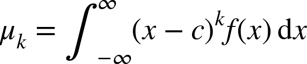
defines the statistical moments. For a known statistical distribution,
the statistical moment is the expectation of order
k around a central point c and
can be evaluated via the following:
gives the cumulative distribution function (or 1 if
over all space), adding in powers of x are what
defines the statistical moments. For a known statistical distribution,
the statistical moment is the expectation of order
k around a central point c and
can be evaluated via the following:
Special quantity, the expectation or average value of x, occurs at c = 0 for the first moment k = 1:

The higher-order moments, k > 1, with respect to this mean are known as the central moments about the mean and are related to descriptive statistics. They are expressed as follows:

The second, third, and fourth central moments about the mean have
useful statistical meanings. We define the variance ![]() as the second moment:
as the second moment:

Its square root is the standard deviation ![]() , a measure of how far the data is distributed from
the mean. The skewness
, a measure of how far the data is distributed from
the mean. The skewness ![]() is a measure of how asymmetric the distribution is
and is related to the third central moment about the mean:
is a measure of how asymmetric the distribution is
and is related to the third central moment about the mean:

The kurtosis is a measure of how fat the tails of the distribution are and is related to the fourth central moment about the mean:

In the next section, we will examine the normal distribution, one of the most useful and ubiquitous probability distributions. The normal distribution has a kurtosis kappa = 3. Because we often compare things to the normal distribution, the term excess kurtosis is defined by the following:

We now define kurtosis (the fatness of the tails) in reference to the normal distribution. Note that many references to the kurtosis are actually referring to the excess kurtosis. The two terms are used interchangeably.
Higher-order moments are possible and have varied usage and applications on the fringe of data science. In this book, we stop at the fourth moment.
Entropy
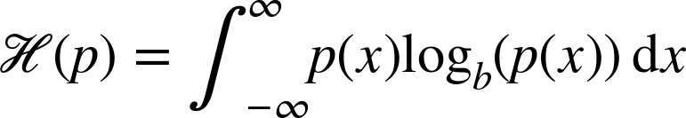
In statistics, entropy is the measure of the unpredictability of the information contained within a distribution. For a continuous distribution, the entropy is as follows:
For a discrete distribution, entropy is shown here:

In an example plot of entropy (Figure 3-2), we see that entropy is lowest when the probability of a 0 or 1 is high, and the entropy is maximal at p = 0.5, where both 0 and 1 are just as likely.

Figure 3-2. Entropy for a Bernoulli distribution
We can also examine the entropy between two distributions by using cross entropy, where p(x) is taken as the true distribution, and q(x) is the test distribution:

And in the discrete case:

Continuous Distributions
Some well-known forms of distributions are well characterized and get frequent use. Many distributions have arisen from real-world observations of natural phenomena. Regardless of whether the variates are described by real or integer numbers, indicating respective continuous and discrete distributions, the basic principles for determining the cumulative probability, statistical moments, and statistical measures are the same.
Uniform
The uniform distribution has a constant probability density over its supported range
![]() , and is zero everywhere else. In fact, this is
just a formal way of describing the random, real-number generator on the interval
, and is zero everywhere else. In fact, this is
just a formal way of describing the random, real-number generator on the interval
[0,1] that you are familiar with, such as
java.util.Random.nextDouble(). The default constructor sets a lower bound
a = 0.0 and an upper bound of
b = 1.0. The probability density of a uniform
distribution is expressed graphically as a top
hat or box shape, as shown in Figure 3-3.

Figure 3-3. Uniform PDF with parameters  and
and 
This has the following mathematical form:

The cumulative distribution function (CDF) looks like Figure 3-4.

Figure 3-4. Uniform CDF with parameters  and
and 
This has the form shown here:

In the uniform distribution, the mean and the variance are not directly specified, but are calculated from the lower and upper bounds with the following:


To invoke the uniform distribution with Java, use the class UniformDistribution(a, b), where the
lower and upper bounds are specified in the constructor. Leaving the
constructor arguments blank invokes the standard uniform distribution,
where a = 0.0 and b =
1.0.
UniformRealDistributiondist=newUniformRealDistribution();doublelowerBound=dist.getSupportLowerBound();// 0.0doubleupperBound=dist.getSupportUpperBound();// 1.0doublemean=dist.getNumericalMean();doublevariance=dist.getNumericalVariance();doublestandardDeviation=Math.sqrt(variance);doubleprobability=dist.density(0.5));doublecumulativeProbability=dist.cumulativeProbability(0.5);doublesample=dist.sample();// e.g., 0.023double[]samples=dist.sample(3);// e.g., {0.145, 0.878, 0.431}
Note that we could reparameterize the uniform distribution with
![]() and
and ![]() , where
, where ![]() is the center point (the mean) and
is the center point (the mean) and ![]() is the distance from the center to either the
lower or upper bound. The variance then becomes
is the distance from the center to either the
lower or upper bound. The variance then becomes ![]() with standard deviation
with standard deviation ![]() . The PDF is then
. The PDF is then

and the CDF is

To express the uniform distribution in this centralized form,
calculate ![]() and
and ![]() and enter them into the constructor:
and enter them into the constructor:
/* initialize centralized uniform with mean = 10 and half-width = 2 */doublemean=10.0doublehw=2.0;doublea=mean-hw;doubleb=mean+hw;UniformRealDistributiondist=newUniformRealDistribution(a,b);
At this point, all of the methods will return the correct results without any further alterations. This reparameterization around the mean can be useful when trying to compare distributions. The centered, uniform distribution is naturally extended by the normal distribution (or other symmetric peaked distributions).
Normal
The most useful and widespread distribution, found in so many diverse use cases, is the normal distribution. Also
known as the Gaussian distribution or the
bell curve, this distribution is symmetric about
a central peak whose width can vary. In many cases when we refer to
something as having an average value with plus or minus a certain
amount, we are referring to the normal distribution. For example, for
exam grades in a classroom, the interpretation is that a few people do
really well and a few people do really badly, but most people are
average or right in the middle. In the normal distribution, the center
of the distribution is the maximum peak and is also the mean of the
distribution, μ. The width is parameterized by
σ and is the standard deviation of the values.
The distribution supports all values of ![]() and is shown in Figure 3-5.
and is shown in Figure 3-5.

Figure 3-5. Normal PDF with parameters  and
and 
The probability density is expressed mathematically as follows:

The cumulative distribution function is shaped like Figure 3-6.

Figure 3-6. Normal CDF with parameters  and
and 
This is expressed with the error function:

This is invoked via Java, where the default constructor creates
the standard normal distribution with ![]() and
and ![]() . Otherwise, pass the parameters μ and
σ to the constructor:
. Otherwise, pass the parameters μ and
σ to the constructor:
/* initialize with default mu=0 and sigma=1 */NormalDistributiondist=newNormalDistribution();doublemu=dist.getMean();// 0.0doublesigma=dist.getStandardDeviation();// 1.0doublemean=dist.getNumericalMean();// 0.0doublevariance=dist.getNumericalVariance();// 1.0doublelowerBound=dist.getSupportLowerBound();// -InfinitydoubleupperBound=dist.getSupportUpperBound();// Infinity/* probability at a point x = 0.0 */doubleprobability=dist.density(0.0);/* calc cum at x=0.0 */doublecumulativeProbability=dist.cumulativeProbability(0.0);doublesample=dist.sample();// 1.0120001doublesamples[]=dist.sample(3);// {.0102, -0.009, 0.011}
Multivariate normal
The normal distribution can be generalized to higher dimensions as the multivariate normal (a.k.a. multinormal) distribution. The variate x and the mean μ are vectors, while the covariance matrix Σ contains the variances on the diagonal and the covariances as i,j pairs. In general, the multivariate normal has a squashed ball shape and is symmetric about the mean. This distribution is perfectly round (or spherical) for unit normals when the covariances are 0 and variances are equivalent. An example of the distribution of random points is shown in Figure 3-7.

Figure 3-7. Random points generated from 2D multinormal distribution
The probability distribution function of a ![]() dimensional multinormal distribution takes the
form
dimensional multinormal distribution takes the
form

Note that if the covariance matrix has a determinant equal to
zero such that ![]() , then f(x) blows up to infinity. Also note that when
, then f(x) blows up to infinity. Also note that when
![]() , it is impossible to calculate the required
inverse of the covariance
, it is impossible to calculate the required
inverse of the covariance ![]() . In this case, the matrix is termed
singular. Apache Commons Math will throw the
following exception if this is the case:
. In this case, the matrix is termed
singular. Apache Commons Math will throw the
following exception if this is the case:
org.apache.commons.math3.linear.SingularMatrixException: matrix is singular
What causes a covariance matrix to become singular? This is a symptom of co-linearity, in which two (or more) variates of the underlying data are identical or linear combinations of each other. In other words, if we have three dimensions and the covariance matrix is singular, it may mean that the distribution of data could be better described in two or even one dimension.
There is no analytical expression for the CDF. It can be attained via numerical integration. However, Apache Commons Math supports only univariate numerical integration.
The multivariate normal takes means and covariance as arrays of doubles, although you can still use
RealVector, RealMatrix, or
Covariance instances with their getData()
methods applied:
double[]means={0.0,0.0,0.0};double[][]covariances={{1.0,0.0,0.0},{0.0,1.0,0.0},{0.0,0.0,1.0}};MultivariateNormalDistributiondist=newMultivariateNormalDistribution(means,covariances);/* probability at point x = {0.0, 0.0, 0.0} */doubleprobability=dist.density(x);// 0.1double[]mn=dist.getMeans();double[]sd=dist.getStandardDeviations();/* returns a RealMatrix but can be converted to doubles */double[][]covar=dist.getCovariances().getData();double[]sample=dist.sample();double[][]samples=dist.sample(3);
Note the special case in which the covariance is a diagonal matrix. This occurs when the variables are
completely independent. The determinant of
Σ is just the product of its diagonal elements
![]() . The inverse of a diagonal matrix is yet another
diagonal matrix with each term expressed as
. The inverse of a diagonal matrix is yet another
diagonal matrix with each term expressed as ![]() . The PDF then reduces to the product of univariate
normals:
. The PDF then reduces to the product of univariate
normals:

As in the case of the unit normal, a unit multivariate normal has a mean vector of 0s and a covariance matrix equal to the identity matrix, a diagonal matrix of 1s.
Log normal
The log normal distribution is related
to the normal distribution when the variate
x is distributed logarithmically—that is,
ln(x) is normally distributed. If we substitute
ln(x) for x in the normal
distribution, we get the log normal distribution. There are some
subtle differences. Because the logarithm is defined only for positive
x, this distribution has support on the interval
![]() , where x > 0. The
distribution is asymmetric with a peak near the smaller values of
x and a long tail stretching, infinitely, to
higher values of x, as shown in Figure 3-8.
, where x > 0. The
distribution is asymmetric with a peak near the smaller values of
x and a long tail stretching, infinitely, to
higher values of x, as shown in Figure 3-8.

Figure 3-8. Log normal PDF with parameters  and
and 
The location (scale) parameter m and the shape parameter s rise to the PDF:

Here, m and s are the respective mean and standard deviation of the logarithmically distributed variate X. The CDF looks like Figure 3-9.

Figure 3-9. Log normal CDF with parameters  and
and 
This has the following form:

Unlike the normal distribution, the m is neither the mean (average value) nor the mode (most likely value or the peak) of the distribution. This is because of the larger number of values stretching off to positive infinity. The mean and variance of X are calculated from the following:


We can invoke a log normal distribution with this:
/* initialize with default m=0 and s=1 */NormalDistributiondist=newNormalDistribution();doublelowerBound=dist.getSupportLowerBound();// 0.0doubleupperBound=dist.getSupportUpperBound();// Infinitydoublescale=dist.getScale();// 0.0doubleshape=dist.getShape():// 1.0doublemean=dist.getNumericalMean();// 1.649doublevariance=dist.getNumericalVariance();// 4.671doubledensity=dist.density(1.0);// 0.3989doublecumulativeProbability=dist.cumulativeProbability(1.0);// 0.5doublesample=dist.sample();// 0.428double[]samples=dist.sample(3);// {0.109, 5.284, 2.032}
Where do we see the log normal distribution? The distribution of ages in a human population, and (sometimes) in particle size distribution. Note that the log normal distribution arises from a multiplicative effect of many independent distributions.
Empirical
In some cases you have data, but do not know the distribution that the data
came from. You can still approximate a distribution with your data and
even calculate probability density, cumulative probability, and random
numbers! The first step in working with an empirical distribution is
to collect the data into bins of equal size spanning the range of the
dataset. The class EmpiricalDistribution can input an
array of doubles or can load a file locally or from a URL. In those
cases, data must be one entry per line:
/* get 2500 random numbers from a standard normal distribution */NormalDistributionnd=newNormalDistribution();double[]data=nd.sample(2500);// default constructor assigns bins = 1000// better to try numPoints / 10EmpiricalDistributiondist=newEmpiricalDistribution(25);dist.load(data);// can also load from file or URL !!!doublelowerBound=dist.getSupportLowerBound();// 0.5doubleupperBound=dist.getSupportUpperBound();// 10.1doublemean=dist.getNumericalMean();// 5.48doublevariance=dist.getNumericalVariance();// 15.032doubledensity=dist.density(1.0);// 0.357doublecumulativeProbability=dist.cumulativeProbability(1.0);// 0.153doublesample=dist.sample();// e.g., 1.396double[]samples=dist.sample(3);// e.g., [10.098, 0.7934, 9.981]
We can plot the data from an empirical distribution as a type of bar chart called a histogram, shown in Figure 3-10.

Figure 3-10. Histogram of random normal with parameters  and
and 
The code for a histogram uses the BarChart plot
from Chapter 1, except that we add the data
directly from the EmpiricalDistribution instance that
contains a List of all the SummaryStatistics
of each bin:
/* for an existing EmpiricalDistribution with loaded data */List<SummaryStatistics>ss=dist.getBinStats();intbinNum=0;for(SummaryStatisticss:ss){/* adding bin counts to the XYChart.Series instance */series.getData().add(newData(Integer.toString(binNum++),s.getN()));}// render histogram with JavaFX BarChart
Discrete Distributions
There are several discrete random-number distributions. These support only integers as values, which are designated by k.
Bernoulli
The Bernoulli distribution is the most basic and perhaps most familiar distribution because it is essentially a coin flip. In a “heads we win, tails we lose” situation, the coin has two possible states: tails (k = 0) and heads (k = 1), where k = 1 is designated to have a probability of success equal to p. If the coin is perfect, then p = 1/2; it is equally likely to get heads as it is tails. But what if the coin is “unfair,” indicating p ≠ 1/2? The probability mass function (PMF) can then be represented as follows:

The cumulative distribution function is shown here:

The mean and variance are calculated with the following:

Note that the Bernoulli distribution is related to the binomial
distribution, where the number of trials equals n
= 1. The Bernoulli distribution is implemented with the class BinomialDistribution(1, p) setting
n = 1:
BinomialDistributiondist=newBinomialDistribution(1,0.5);intlowerBound=dist.getSupportLowerBound();// 0intupperBound=dist.getSupportUpperBound();// 1intnumTrials=dist.getNumberOfTrials();// 1doubleprobSuccess=dist.getProbabilityOfSuccess();// 0.5doublemean=dist.getNumericalMean();// 0.5doublevariance=dist.getNumericalVariance();// 0.25// k = 1doubleprobability=dist.probability(1);// 0.5doublecumulativeProbability=dist.cumulativeProbability(1);// 1.0intsample=dist.sample();// e.g., 1int[]samples=dist.sample(3);// e.g., [1, 0, 1]
Binomial
If we perform multiple Bernoulli trials, we arrive at the binomial distribution. For n Bernoulli trials, each with probability of success p, the distribution of successes k has the form in Figure 3-11.

Figure 3-11. Binomial PMF with parameters  and
and 
The probability mass function is expressed with the following:

The CDF looks like Figure 3-12.

Figure 3-12. Binomial CDF with parameters  and
and 
The CDF takes the form

I1-p is the regularized incomplete beta function. The mean and variance are computed via the following:

In Java, BinomialDistribution has two required arguments in the constructor:
n, the number of trials; and
p, the probability of success for one trial:
BinomialDistributiondist=newBinomialDistribution(10,0.5);intlowerBound=dist.getSupportLowerBound();// 0intupperBound=dist.getSupportUpperBound();// 10intnumTrials=dist.getNumberOfTrials();// 10doubleprobSuccess=dist.getProbabilityOfSuccess();// 0.5doublemean=dist.getNumericalMean();// 5.0doublevariance=dist.getNumericalVariance();// 2.5// k = 1doubleprobability=dist.probability(1);// 0.00977doublecumulativeProbability=dist.cumulativeProbability(1);// 0.0107intsample=dist.sample();// e.g., 9int[]samples=dist.sample(3);// e.g., [4, 5, 4]
Poisson
The Poisson distribution is often
used to describe discrete, independent events that occur
rarely. The number of events are the integers ![]() that occur over some interval with a constant rate
that occur over some interval with a constant rate
![]() gives rise to the PMF in Figure 3-13.
gives rise to the PMF in Figure 3-13.

Figure 3-13. Poisson PMF with parameters 
The form of the PMF is

Figure 3-14 shows the CDF.

Figure 3-14. Poisson CDF with parameters 
The CDF is expressed via

The mean and variance are both equivalent to the rate parameter
![]() as
as

The Poisson is implemented with the parameter ![]() in the constructor and has an upper bound
at
in the constructor and has an upper bound
at Integer.MAX k =
232 – 1 = 2147483647:
PoissonDistributiondist=newPoissonDistribution(3.0);intlowerBound=dist.getSupportLowerBound();// 0intupperBound=dist.getSupportUpperBound();// 2147483647doublemean=dist.getNumericalMean();// 3.0doublevariance=dist.getNumericalVariance();// 3.0// k = 1doubleprobability=dist.probability(1);// 0.1494doublecumulativeProbability=dist.cumulativeProbability(1);// 0.1991intsample=dist.sample();// e.g., 1int[]samples=dist.sample(3);// e.g., [2, 4, 1]
Characterizing Datasets
Once we have a dataset, the first thing we should do is understand the character of the data. We should know the numerical limits, whether any outliers exist, and whether the data has a shape like one of the known distribution functions. Even if we have no idea what the underlying distribution is, we can still check whether two separate datasets come from the same (unknown) distribution. We can also check how related (or unrelated) each pair of variates is via covariance/correlation. If our variate x comes with a response y, we can check a linear regression to see whether the most basic of relationships exists between x and y. Most of the classes in this section are best for small, static datasets that can fit entirely into memory, because most of the methods in these classes rely on stored data. In the following section, we deal with data that is so large (or inconvenient) that it cannot fit in memory.
Calculating Moments
In the previous section where we discussed statistical moments, formulas were presented for calculating moments and their various statistical outcomes when we know the probability distribution function f(x). When dealing with real data, we usually do not know the form of f(x) and so we must estimate the moments numerically. The moment calculations have another critical feature: robustness. Estimating statistical quantities can result in numerical error as extreme values are encountered. Using the method of updating moments, we can avoid numerical imprecision.


Updating moments
Without the factor 1/n for the estimate of the central moment, the form is as follows:

In this particular form, the unnormalized moments can be split into parts via straightforward calculations. This gives us a great advantage that the unnormalized moments can be calculated in parts, perhaps in different processes or even on different machines entirely, and we can glue back together the pieces later. Another advantage is that this formulation is less sensitive to extreme values. The combined unnormalized central moment for the two chunks is shown here:

![]() is the difference between the means of the two
data chunks. Of course, you will also need a method for merging the
means, because this formula is applicable only for
k > 1. Given any two data chunks with known
means and counts, the total count is
is the difference between the means of the two
data chunks. Of course, you will also need a method for merging the
means, because this formula is applicable only for
k > 1. Given any two data chunks with known
means and counts, the total count is ![]() , and the mean is robustly calculated as
follows:
, and the mean is robustly calculated as
follows:

If one of the data chunks has only one point x, then the formulation for combining the unnormalized central moments is simplified:

Here, ![]() is the difference between the added value
x and the mean value of the existing data
chunk.
is the difference between the added value
x and the mean value of the existing data
chunk.
In the next section, we will see how these formulas are used to robustly calculate important properties to statistics. They become essential in distributed computing applications when we wish to break statistical calculations into many parts. Another useful application is storeless calculations in which, instead of performing calculations on whole arrays of data, we keep track of moments as we go, and update them incrementally.
Descriptive Statistics
We instantiate DescriptiveStatistics with no
argument to add values later, or start it out with an array of doubles
(and then can still add values later). Although you can use StatUtils static methods, this is not
Java-like, and although there is nothing wrong with it, it’s probably
wiser to use DescriptiveStatistics instead. Some of the
formulas in this section are not stable, and a more robust method is
described in the next section. Indeed, some of those methods are used in
the descriptive stats methods as well. In Table 3-1,
we display the data from Anscombe’s quartet for further analysis in this chapter.
| x1 | y1 | x2 | y2 | x3 | y3 | x4 | y4 |
|---|---|---|---|---|---|---|---|
| 10.0 | 8.04 | 10.0 | 9.14 | 10.0 | 7.46 | 8.0 | 6.58 |
| 8.0 | 6.95 | 8.0 | 8.14 | 8.0 | 6.77 | 8.0 | 5.76 |
| 13.0 | 7.58 | 13.0 | 8.74 | 13.0 | 12.74 | 8.0 | 7.71 |
| 9.0 | 8.81 | 9.0 | 8.77 | 9.0 | 7.11 | 8.0 | 8.84 |
| 11.0 | 8.33 | 11.0 | 9.26 | 11.0 | 7.81 | 8.0 | 8.47 |
| 14.0 | 9.96 | 14.0 | 8.10 | 14.0 | 8.84 | 8.0 | 7.04 |
| 6.0 | 7.24 | 6.0 | 6.13 | 6.0 | 6.08 | 8.0 | 5.25 |
| 4.0 | 4.26 | 4.0 | 3.10 | 4.0 | 5.39 | 19.0 | 12.50 |
| 12.0 | 10.84 | 12.0 | 9.13 | 12.0 | 8.15 | 8.0 | 5.56 |
| 7.0 | 4.82 | 7.0 | 7.26 | 7.0 | 6.42 | 8.0 | 7.91 |
| 5.0 | 5.68 | 5.0 | 4.74 | 5.0 | 5.73 | 8.0 | 6.89 |
We can then create DescriptiveStatistics classes with
these datasets:
/* stats for Anscombe's y1 */DescriptiveStatisticsdescriptiveStatistics=newDescriptiveStatistics();descriptiveStatistics.addValue(8.04);descriptiveStatistics.addValue(6.95);//keep adding y1 values
However, you may already have all the data that you need, or maybe
it’s just an initial set that you will add to later. You can always add
more values with ds.addValue(double value) if needed. At
this point, you can display a report of stats with either a call to the
method, or by printing the class directly:
System.out.println(descriptiveStatistics);
This produces the following result:
DescriptiveStatistics:
n: 11
min: 4.26
max: 10.84
mean: 7.500909090909091
std dev: 2.031568135925815
median: 7.58
skewness: -0.06503554811157437
kurtosis: -0.5348977343727395
All of these quantities (and more) are available via their specific getters, as explained next.
Mean
The average value of the sample or mean is calculated directly:

However, this calculation is sensitive to extreme values, and
given ![]() , the mean can be updated for each added value
x:
, the mean can be updated for each added value
x:

Commons Math uses the update formula for mean calculation
when the getMean() method is called:
doublemean=descriptiveStatistics.getMean();
Median
The middle value of a sorted (ascending) dataset is the median. The advantage is that it minimizes the problem of extreme values. While there is no direct calculation of the median in Apache Commons Math, it is easy to calculate by taking the average of the two middle members if the array length is even; and otherwise, just return the middle member of the array:
// sort the stored valuesdouble[]sorted=descriptiveStatistics.getSortedValues();intn=sorted.length;doublemedian=(n%2==0)?(sorted[n/2-1]+sorted[n/2])/2.0:sorted[n/2];
Mode
The mode is the most likely value. The concept of
mode does not make sense if the values are
doubles, because there is probably only one of each. Obviously, there
will be exceptions (e.g., when many zeros occur) or if the dataset is
large and the numerical precision is small (e.g., two decimal places).
The mode has two use cases then: if the variate being considered is
discrete (integer), then the mode can be useful, as in dataset four of
Anscombe’s quartet. Otherwise, if you have created bins from empirical
distribution, the mode is the max bin. However, you should consider
the possibility that your data is noisy and the bin counts may
erroneously identify an outlier as a mode.The StatUtils
class contains several static methods useful for statistics.
Here we utilize its mode method:
// if there is only one max, it's stored in mode[0]// if there is more than one value that has equally high counts// then values are stored in mode in ascending orderdouble[]mode=StatUtils.mode(x4);//mode[0] = 8.0double[]test={1.0,2.0,2.0,3.0,3.0,4.0}//mode[0] = 2.0//mode[1] = 3.0
Variance
The variance is a measure of how much the data is spread out and is always a positive, real number greater than or equal to zero. If all values of x are equal, the variance will be zero. Conversely, a larger spread of numbers will correspond to a larger variance. The variance of a known population of data points is equivalent to the second central moment about the mean and is expressed as follows:

However, most of the time we do not have all of the data—we are only sampling from a larger (possibly unknown) dataset and so a correction for this bias is needed:

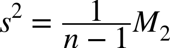
This form is known as the sample variance and is most often the variance we will use. You may note that the sample variance can be expressed in terms of the second-order, unnormalized moment:
As with the mean calculation, the Commons Math variance is
calculated using the update formula for the second unnormalized moment
for a new data point ![]() , an existing mean
, an existing mean ![]() and the newly updated mean
and the newly updated mean ![]() :
:

Here, ![]() .
.
Most of the time when the variance is required, we are asking for the bias-corrected, sample variance because our data is usually a sample from some larger, possibly unknown, set of data:
doublevariance=descriptiveStatistics.getVariance()
However, it is also straightforward to retrieve the population variance if it is required:
doublepopulationVariance=descriptiveStatistics.getPopulationVariance();
Standard deviation
The variance is difficult to visualize because it is on the order of x2 and usually a large number compared to the mean. By taking the square root of the variance, we define this as the standard deviation s. This has the advantage of being in the same units of the variates and the mean. It is therefore helpful to use things like μ +– σ, which can indicate how much the data deviates from the mean. The standard deviation can be explicitly calculated with this:
However, in practice, we use the update formulas to calculate the sample variance, returning the standard deviation as the square root of the sample variance when required:
doublestandardDeviation=descriptiveStatistics.getStandardDeviation();
Should you require the population standard deviation, you can calculate this directly by taking the square root of the population variance.
Error on the mean
While it is often assumed that the standard deviation is the error on the mean, this is not true. The standard deviation describes how the data is spread around the average. To calculate the accuracy of the mean itself, sx, we use the standard deviation:

doublemeanErr=descriptiveStatistics.getStandardDeviation()/Math.sqrt(descriptiveStatistics.getN());
Skewness
The skewness measures how asymmetrically distributed the data is and can be either a positive or negative real number. A positive skew signifies that most of the values leans toward the origin (x = 0), while a negative skew implies the values are distributed away (to right). A skewness of 0 indicates that the data is perfectly distributed on either side of the data distribution'’s peak value. The skewness can be calculated explicitly as follows:

However, a more robust calculation of the skewness is achieved by updating the third central moment:

Then you calculate the skewness when it is called for:

The Commons Math implementation iterates over the stored dataset, incrementally updating M3 and then performing the bias correction, and returns the skewness:
doubleskewness=descriptiveStatistics.getSkewness();
Kurtosis
The kurtosis is a measure of how “tailed” a distribution of data is. The sample kurtosis estimate is related to the fourth central moment about the mean and is calculated as shown here:

This can be simplified as follows:

A kurtosis at or near 0 signifies that the data distribution is extremely narrow. As the kurtosis increases, extreme values coincide with long tails. However, we often want to express the kurtosis as related to the normal distribution (which has a kurtosis = 3). We can then subtract this part and call the new quantity the excess kurtosis, although in practice most people just refer to the excess kurtosis as the kurtosis. In this definition, κ = 0 implies that the data has the same peak and tail shape as a normal distribution. A kurtosis higher than 3 is called leptokurtic and has wider tails than a normal distribution. When κ is less than 3, the distribution is said to be platykurtic and the distribution has few values in the tail (less than the normal distribution). The excess kurtosis calculation is as follows:

As in the case for the variance and skewness, the kurtosis is calculated by updating the fourth unnormalized central moment. For each point added to the calculation, M4 can be updated with the following equation as long as the number of points n >= 4. At any point, the skew can be computed from the current value of M4:

The default calculation returned by getKurtosis is
the excess kurtosis definition. This can be checked by implementing the class
org.apache.commons.math3.stat.descriptive.moment.Kurtosis,
which is called by getKurtosis():
doublekurtosis=descriptiveStatistics.getKurtosis();
Multivariate Statistics
So far, we have addressed the situation where we are concerned with
one variate at a time. The class DescriptiveStatistics
takes only one-dimensional data. However, we usually have several
dimensions, and it is not uncommon to have hundreds of dimensions. There
are two options: the first is to use the
MultivariateStatisticalSummary class, which is described in the next section. If you can live
without skewness and kurtosis, that is your best option. If you do
require the full set of statistical quantities, your best bet is to
implement a Collection instance of
DescriptiveStatistics objects. First consider what you want
to keep track of. For example, in the case of Anscombe’s quartet, we can collect univariate
statistics with the following:
DescriptiveStatisticsdescriptiveStatisticsX1=newDescriptiveStatistics(x1);DescriptiveStatisticsdescriptiveStatisticsX2=newDescriptiveStatistics(x2);...List<DescriptiveStatistics>dsList=newArrayList<>();dsList.add(descriptiveStatisticsX1);dsList.add(descriptiveStatisticsX2);...
You can then iterate through the List, calling statistical quantities or
even the raw data:
for(DescriptiveStatisticsds:dsList){double[]data=ds.getValues();// do something with data ordoublekurtosis=ds.getKurtosis();// do something with kurtosis}
If the dataset is more complex and you know you will need to call
specific columns of data in your ensuing analysis, use Map instead:
DescriptiveStatisticsdescriptiveStatisticsX1=newDescriptiveStatistics(x1);DescriptiveStatisticsdescriptiveStatisticsY1=newDescriptiveStatistics(y1);DescriptiveStatisticsdescriptiveStatisticsX2=newDescriptiveStatistics(x2);Map<String,DescriptiveStatistics>dsMap=newHashMap<>();dsMap.put("x1",descriptiveStatisticsX1);dsMap.put("y1",descriptiveStatisticsY1);dsMap.put("x2",descriptiveStatisticsX2);
Of course, now it is trivial to call a specific quantity or dataset by its key:
doublex1Skewness=dsMap.get("x1").getSkewness();double[]x1Values=dsMap.get("x1").getValues();
This will become cumbersome for a large number of dimensions, but
you can simplify this process if the data was already stored in
multidimensional arrays (or matrices) where you loop over the column
index. Also, you may have already stored your data in the
List or Map of the data container classes, so
automating the process of building a multivariate
Collection of DescriptiveStatistics objects
will be straightforward. This is particularly efficient if you already
have a data dictionary (a list of variable names and their properties)
from which to iterate over. If you have high-dimensional numeric data of
one type and it already exists in a matrix of double array form, it
might be easier to use the MultivariateSummaryStatistics
class in the next section.
Covariance and Correlation
The covariance and correlation matrices are symmetric, square m × m matrices with dimension m equal to the number columns in the original dataset.
Covariance
The covariance is the two-dimensional equivalent of the variance. It measures how two variates, in combination, differ from their means. It is calculated as shown here:

Just as in the case of the one-dimensional, statistical sample moments, we note that the quantity

can be expressed as an incremental update to the co-moment of the pair of variables xi and xj, given a known means and counts for the existing dimensions:

Then the covariance can be calculated at any point:

The code to calculate the covariance is shown here:
Covariancecov=newCovariance();/* examples using Anscombe's Quartet data */doublecov1=cov.covariance(x1,y1);// 5.501doublecov2=cov.covariance(x2,y2);// 5.499doublecov3=cov.covariance(x3,y3);// 5.497doublecov4=cov.covariance(x4,y5);// 5.499
If you already have the data in a 2D array of doubles or a
RealMatrix instance, you can pass them directly to the
constructor like this:
// double[][] myData or RealMatrix myDataCovariancecovObj=newCovariance(myData);// cov contains covariances and can be accessed// from RealMatrix.get(i,j) retrieve elementsRealMatrixcov=covObj.getCovarianceMatrix();
Note that the diagonal of the covariance matrix ![]() is just the variance of column
i and therefore the square root of the diagonal
of the covariance matrix is the standard deviation of each dimension
of data. Because the population mean is usually not known, we use the
biased covariance with the sample mean. If we did know the population
mean, the unbiased correction factor 1/n would be
used to calculate the unbiased covariance:
is just the variance of column
i and therefore the square root of the diagonal
of the covariance matrix is the standard deviation of each dimension
of data. Because the population mean is usually not known, we use the
biased covariance with the sample mean. If we did know the population
mean, the unbiased correction factor 1/n would be
used to calculate the unbiased covariance:
Pearson’s correlation
The Pearson correlation coefficient is related to covariance via the following, and is a measure of how likely two variates are to vary together:

The correlation coefficient takes a value between –1 and 1, where 1 indicates that the two variates are nearly identical. –1 indicates that they are opposites. In Java, there are once again two options, but using the default constructor, we get this:
PearsonsCorrelationcorr=newPearsonsCorrelation();/* examples using Anscombe's Quartet data */doublecorr1=corr.correlation(x1,y1));// 0.816doublecorr2=corr.correlation(x2,y2));// 0.816doublecorr3=corr.correlation(x3,y3));// 0.816doublecorr4=corr.correlation(x4,y4));// 0.816
However, if we already have data, or a Covariance
instance, we can use the following:
// existing Covariance covPearsonsCorrelationcorrObj=newPearsonsCorrelation(cov);// double[][] myData or RealMatrix myDataPearsonsCorrelationcorrObj=newPearsonsCorrelation(myData);// from RealMatrix.get(i,j) retrieve elementsRealMatrixcorr=corrObj.getCorrelationMatrix();
Warning
Correlation is not causation! One of the dangers in statistics is the interpretation of correlation. When two variates have a high correlation, we tend to assume that this implies that one variable is responsible for causing the other. This is not the case. In fact, all you can assume is that you can reject the idea that the variates have nothing to do with each other. You should view correlation as a fortunate coincidence, not a foundational basis for the underlying behavior of the system being studied.
Regression
Often we want to find the relationship between our variates
X and their responses ![]() . We are trying to find a set of values for
. We are trying to find a set of values for
![]() such that y = X
such that y = X![]() . In the end, we want three things: the parameters,
their errors, and a statistic of how good the fit is,
. In the end, we want three things: the parameters,
their errors, and a statistic of how good the fit is, ![]() .
.
Simple regression
If X has only one dimension, the problem is the familiar equation of a
line ![]() , and the problem can be classified as simple
regression. By calculating
, and the problem can be classified as simple
regression. By calculating ![]() , the variance of
, the variance of ![]() and
and ![]() , and the covariance between
, and the covariance between ![]() and
and ![]() , we can estimate the slope:
, we can estimate the slope:

Then, using the slope and the means of x and y, we can estimate the intercept:

The code in Java uses the SimpleRegression class:
SimpleRegressionrg=newSimpleRegression();/* x-y pairs of Anscombe's x1 and y1 */double[][]xyData={{10.0,8.04},{8.0,6.95},{13.0,7.58},{9.0,8.81},{11.0,8.33},{14.0,9.96},{6.0,7.24},{4.0,4.26},{12.0,10.84},{7.0,4.82},{5.0,5.68}};rg.addData(xyData);/* get regression results */doublealpha=rg.getIntercept();// 3.0doublealpha_err=rg.getInterceptStdErr();// 1.12doublebeta=rg.getSlope();// 0.5doublebeta_err=rg.getSlopeStdErr();// 0.12doubler2=rg.getRSquare();// 0.67
We can then interpret these results as ![]() , or more specifically as
, or more specifically as ![]() . How much can we trust this model? With
. How much can we trust this model? With
![]() , it’s a fairly decent fit, but the closer it is to
the ideal of
, it’s a fairly decent fit, but the closer it is to
the ideal of ![]() , the better. Note that if we perform the same
regression on the other three datasets from Anscombe’s quartet, we get
identical parameters, errors, and
, the better. Note that if we perform the same
regression on the other three datasets from Anscombe’s quartet, we get
identical parameters, errors, and ![]() . This is a profound, albeit perplexing, result.
Clearly, the four datasets look different, but their linear fits (the
superposed blue lines) are identical. Although linear regression is a
powerful yet simple method for understanding our data as in case 1, in
case 2 linear regression in x is probably the
wrong tool to use here. In case 3, linear regression is probably the
right tool, but we could sensor (remove) the data point that appears
to be an outlier. In case 4, a regression model is most likely not
appropriate at all. This does demonstrate how easy it is to fool
ourselves that a model is correct if we look at only a few parameters
after blindly throwing data into an analysis method.
. This is a profound, albeit perplexing, result.
Clearly, the four datasets look different, but their linear fits (the
superposed blue lines) are identical. Although linear regression is a
powerful yet simple method for understanding our data as in case 1, in
case 2 linear regression in x is probably the
wrong tool to use here. In case 3, linear regression is probably the
right tool, but we could sensor (remove) the data point that appears
to be an outlier. In case 4, a regression model is most likely not
appropriate at all. This does demonstrate how easy it is to fool
ourselves that a model is correct if we look at only a few parameters
after blindly throwing data into an analysis method.
Multiple regression
There are many ways to solve this problem, but the most common and probably most useful is the ordinary least squares (OLS) method. The solution is expressed in terms of linear algebra:

The OLSMultipleLinearRegression class in Apache Commons Math is just a convenient wrapper
around a QR decomposition. This implementation also provides
additional functions beyond the QR decomposition that you will find
useful. In particular, the variance-covariance matrix of
![]() is as follows, where the matrix
R is from the QR decomposition:
is as follows, where the matrix
R is from the QR decomposition:

In this case, R must be truncated to the
dimension of beta. Given the fit residuals ![]() , we can calculate the variance of the errors
, we can calculate the variance of the errors
![]() where
where ![]() and
and ![]() are the respective number of rows and columns of
are the respective number of rows and columns of
![]() . The square root of the diagonal values of
. The square root of the diagonal values of
![]() times the constant
times the constant ![]() gives us the estimate of errors on the fit parameters:
gives us the estimate of errors on the fit parameters:

The Apache Commons Math implementation of ordinary least squares regression utilizes the QR decomposition covered in linear algebra. The methods in the example code are convenient wrappers around several standard matrix operations. Note that the default is to include an intercept term, and the corresponding value is the first position of the estimated parameters:
double[][]xNData={{0,0.5},{1,1.2},{2,2.5},{3,3.6}};double[]yNData={-1,0.2,0.9,2.1};// default is to include an interceptOLSMultipleLinearRegressionmr=newOLSMultipleLinearRegression();/* NOTE that y and x are reversed compared to other classes / methods */mr.newSampleData(yNData,xNData);double[]beta=mr.estimateRegressionParameters();// [-0.7499, 1.588, -0.5555]double[]errs=mr.estimateRegressionParametersStandardErrors();// [0.2635, 0.6626, 0.6211]doubler2=mr.calculateRSquared();// 0.9945
Linear regression is a vast topic with many adaptations—too many to be covered here. However, it is worth noting that these methods are relevant only if the relations between X and y are actually linear. Nature is full of nonlinear relationships, and in Chapter 5 we will address more ways of exploring these.
Working with Large Datasets
When our data is so large that it is inefficient to store it in memory (or it
just won’t fit!), we need an alternative method of calculating statistical
measures. Classes such as DescriptiveStatistics store all
data in memory for the duration of the instantiated class. However,
another way to attack this problem is to store only the unnormalized
statistical moments and update them one data point at a time, discarding
that data point after it has been assimilated into the calculations.
Apache Commons Math has two such classes: SummaryStatistics and
MultivariateSummaryStatistics.
The usefulness of this method is enhanced by the fact that we
can also sum unnormalized moments in parallel. We can split data into
partitions and keep track of moments in each partition as we add one value
at a time. In the end, we can merge all those moments and then find the
summary statistics. The Apache Commons Math class
AggregateSummaryStatistics takes care of this. It is easy to imagine terabytes of data
distributed over a large cluster in which each node is updating
statistical moments. As the jobs complete, the moments can be merged in a
simple calculation, and the task is complete.
In general, a dataset X can be partitioned into ![]() smaller datasets: X1, X2,
smaller datasets: X1, X2, ![]() Xk. Ideally, we can perform all sorts of computations on
each partition Xi and then later merge these results to get the desired
quantities for X. For example, if we wanted to count the number of data
points in X, we could count the number of points in each subset
and then later add those results together to get the total count:
Xk. Ideally, we can perform all sorts of computations on
each partition Xi and then later merge these results to get the desired
quantities for X. For example, if we wanted to count the number of data
points in X, we could count the number of points in each subset
and then later add those results together to get the total count:

This is true whether the partitions were calculated on the same machine in different threads, or on different machines entirely.
So if we calculated the number of points, and additionally, the sum of values for each subset (and kept track of them), we could later use that information to calculate the mean of X in a distributed way.

At the simplest level, we need only computations for pairwise
operations, because any number of operations can reduce that way. For
example, X = (X1 + X2) + (X3 + X4) is a combination of three pairwise operations. There
are then three general situations for pairwise algorithms: first, where we
are merging two partitions, each with ![]() ; the second, where one partition has
; the second, where one partition has ![]() and the other partition is a singleton with
and the other partition is a singleton with
![]() ; and the third where both partitions are
singletons.
; and the third where both partitions are
singletons.
Accumulating Statistics
We saw in the preceding chapter how stats can be updated. Perhaps it
occurred to you that we could calculate and store the (unnormalized)
moments on different machines at different times, and update them at
our convenience. As long as you keep track of the number of points and
all relevant statistical moments, you
can recall those at any time and update them with a new set of data
points. While the DescriptiveStatistics class stored all
the data and did these updates in one long chain of calculations, the
SummaryStatistics class (and
MultivariateSummaryStatistics class) do not store any of
the data you input to them. Rather, these classes store only the relevant
![]() ,
, ![]() , and
, and ![]() . For massive datasets, this is an efficient way to keep track of stats without incurring the huge costs of storage or
processing power whenever we need a statistic such as mean or standard
deviation.
. For massive datasets, this is an efficient way to keep track of stats without incurring the huge costs of storage or
processing power whenever we need a statistic such as mean or standard
deviation.
SummaryStatisticsss=newSummaryStatistics();/* This class is storeless, so it is optimized to take one value at a time */ss.addValue(1.0);ss.addValue(11.0);ss.addValue(5.0);/* prints a report */System.out.println(ss);
As with the DescriptiveStatistics class, the
SummaryStatistics class also has a toString()
method that prints a nicely formatted report:
SummaryStatistics:
n: 3
min: 1.0
max: 11.0
sum: 17.0
mean: 5.666666666666667
geometric mean: 3.8029524607613916
variance: 25.333333333333332
population variance: 16.88888888888889
second moment: 50.666666666666664
sum of squares: 147.0
standard deviation: 5.033222956847166
sum of logs: 4.007333185232471
For multivariate statistics, the
MultivariateSummaryStatistics class is directly analogous to its
univariate counterpart. To instantiate this class, you must specify the
dimension of the variates (the number of columns in the dataset) and
indicate whether the input data is a sample. Typically, this option
should be set to true, but note that if you forget it, the
default is false, and that will have consequences. The
MultivariateSummaryStatistics class contains methods that
keep track of the covariance between every set of variates. Setting the
constructor argument isCovarianceBiasedCorrected to
true uses the biased correction factor for the
covariance:
MultivariateSummaryStatisticsmss=newMultivariateSummaryStatistics(3,true);/* data could be 2d array, matrix, or class with a double array data field */double[]x1={1.0,2.0,1.2};double[]x2={11.0,21.0,10.2};double[]x3={5.0,7.0,0.2};/* This class is storeless, so it is optimized to take one value at a time */mss.addValue(x1);mss.addValue(x2);mss.addValue(x3);/* prints a report */System.out.println(mss);
As in SummaryStatistics, we can print a formatted
report with the added bonus of the covariance matrix:
MultivariateSummaryStatistics:
n: 3
min: 1.0, 2.0, 0.2
max: 11.0, 21.0, 10.2
mean: 5.666666666666667, 10.0, 3.866666666666667
geometric mean: 3.8029524607613916, 6.649399761150975, 1.3477328201610665
sum of squares: 147.0, 494.0, 105.52
sum of logarithms: 4.007333185232471, 5.683579767338681, 0.8952713646500794
standard deviation: 5.033222956847166, 9.848857801796104, 5.507570547286103
covariance: Array2DRowRealMatrix{{25.3333333333,49.0,24.3333333333},
{49.0,97.0,51.0},{24.3333333333,51.0,30.3333333333}}
Of course, each of these quantities is accessible via their getters:
intd=mss.getDimension();longn=mss.getDimension();double[]min=mss.getMin();double[]max=mss.getMax();double[]mean=mss.getMean();double[]std=mss.getStandardDeviation();RealMatrixcov=mss.getCovariance();
Note
At this time, third- and fourth-order moments are not calculated
in SummaryStatistics and
MultivariateSummaryStatistics classes, so skewness and
kurtosis are not available. They are in the works!
Merging Statistics
The unnormalized statistical moments and co-moments can also be merged. This is useful when data partitions are processed in parallel and the results are merged later when all subprocesses have completed.
For this task, we use the class AggregateSummaryStatistics. In
general, statistical moments propagate as the order is increased. In
other words, in order to calculate the third moment ![]() you will need the moments
you will need the moments ![]() and
and ![]() . It is therefore essential to calculate and update
the highest order moment first and then work downward.
. It is therefore essential to calculate and update
the highest order moment first and then work downward.
For example, after calculating the quantity ![]() as described earlier, update
as described earlier, update ![]() with
with

Then update ![]() with
with

Next, update ![]() with:
with:

And finally, update the mean with:

Note that these update formulas are for merging data partitions
where both have ![]() . If either of the partitions is a singleton
(
. If either of the partitions is a singleton
(![]() ), then use the incremental update formulas from the
prior section.
), then use the incremental update formulas from the
prior section.
Here is an example demonstrating the aggregation of independent
statistical summaries. Note that here, any instance of
SummaryStatistics could be serialized and stored away for
future use.
// The following three summaries could occur on// three different machines at different timesSummaryStatisticsss1=newSummaryStatistics();ss1.addValue(1.0);ss1.addValue(11.0);ss1.addValue(5.0);SummaryStatisticsss2=newSummaryStatistics();ss2.addValue(2.0);ss2.addValue(12.0);ss2.addValue(6.0);SummaryStatisticsss3=newSummaryStatistics();ss3.addValue(0.0);ss3.addValue(10.0);ss3.addValue(4.0);// The following can occur on any machine at// any time later than aboveList<SummaryStatistics>ls=newArrayList<>();ls.add(ss1);ls.add(ss2);ls.add(ss3);StatisticalSummaryValuess=AggregateSummaryStatistics.aggregate(ls);System.out.println(s);
This prints the following report as if the computation had occurred on a single dataset:
StatisticalSummaryValues:
n: 9
min: 0.0
max: 12.0
mean: 5.666666666666667
std dev: 4.444097208657794
variance: 19.75
sum: 51.0
Regression
The SimpleRegression class makes this easy, because moments and co-moments add
together easily. The Aggregates statistics produce the same result as in
the original statistical summary:.
SimpleRegressionrg=newSimpleRegression();/* x-y pairs of Anscombe's x1 and y1 */double[][]xyData={{10.0,8.04},{8.0,6.95},{13.0,7.58},{9.0,8.81},{11.0,8.33},{14.0,9.96},{6.0,7.24},{4.0,4.26},{12.0,10.84},{7.0,4.82},{5.0,5.68}};rg.addData(xyData);/**/double[][]xyData2={{10.0,8.04},{8.0,6.95},{13.0,7.58},{9.0,8.81},{11.0,8.33},{14.0,9.96},{6.0,7.24},{4.0,4.26},{12.0,10.84},{7.0,4.82},{5.0,5.68}};SimpleRegressionrg2=newSimpleRegression();rg2.addData(xyData);/* merge the regression from rg with rg2 */rg.append(rg2);/* get regression results for the combined regressions */doublealpha=rg.getIntercept();// 3.0doublealpha_err=rg.getInterceptStdErr();// 1.12doublebeta=rg.getSlope();// 0.5doublebeta_err=rg.getSlopeStdErr();// 0.12doubler2=rg.getRSquare();// 0.67
In the case of multivariate regression,
MillerUpdatingRegression enables a storeless regression via
MillerUpdatingRegression.addObservation(double[] x, double
      y)
or MillerUpdatingRegression.addObservations(double[][]
x, double[] y).
intnumVars=3;booleanincludeIntercept=true;MillerUpdatingRegressionr=newMillerUpdatingRegression(numVars,includeIntercept);double[][]x={{0,0.5},{1,1.2},{2,2.5},{3,3.6}};double[]y={-1,0.2,0.9,2.1};r.addObservations(x,y);RegressionResultsrr=r.regress();double[]params=rr.getParameterEstimates();double[]errs=rr.getStdErrorOfEstimates();doubler2=rr.getRSquared();
Using Built-in Database Functions
Most databases have built-in statistical aggregation functions. If your
data is already in MySQL you may not have to import the data to a Java
application. You can use built-in functions. The use of GROUP
BY and ORDER BY combined with a WHERE
clause make this a powerful way to reduce your data to statistical
summaries. Keep in mind that the computation must be done somewhere,
either in your application or by the database server. The trade-off is, is
the data small enough that I/O and CPU is not an issue? If you don’t want
the DB performance to take a hit CPU-wise, exploiting all that I/O
bandwidth might be OK. Other times, you would rather have the CPU in the
DB app compute all the stats and use just a tiny bit of I/O to shuttle
back the results to the waiting app.
Warning
In MySQL, the built-in function STDDEV returns
the population’s standard deviation. Use the more specific
functions STDDEV_SAMP and
STDDEV_POP for respective sample and population standard
deviations.
For example, we can query a table with various built-in functions, which in this case are example revenue statistics such as AVG and STDDEV from a sales table:
SELECTcity,SUM(revenue)AStotal_rev,AVG(revenue)ASavg_rev,STDDEV(revenue)ASstd_revFROMsales_tableWHERE<somecriteria>GROUPBYcityORDERBYtotal_revDESC;
Note that we can use the results as is from a JDBC query or dump
them directly into the constructor of StatisticalSummaryValues(double mean,
double variance, long count, double min, double max) for further
use down the line. Say we have a query like this:
SELECTcity,AVG(revenue)ASavg_rev,VAR_SAMP(revenue)ASvar_rev,COUNT(revenue)AScount_rev,MIN(revenue)ASmin_rev,MAX(revenue)ASmax_revFROMsales_tableWHERE<somecriteria>GROUPBYcity;
We can populate each StatistialSummaryValues instance
(arbitrarily) in a List or Map with keys equal to
city as we iterate through the database cursor:
Map<String,StatisticalSummaryValues>revenueStats=newHashMap<>();Statementst=c.createStatement();ResultSetrs=st.executeQuery(selectSQL);while(rs.next()){StatisticalSummaryValuesss=newStatisticalSummaryValues(rs.getDouble("avg_rev"),rs.getDouble("var_rev"),rs.getLong("count_rev"),rs.getDouble("min_rev"),rs.getDouble("max_rev"));revenueStats.put(rs.getString("city"),ss);}rs.close();st.close();
Some simple database wizardry can save lots of I/O for larger datasets.