Chapter 5. Hyperparameter Optimization
Training a deep model and training a good deep model are very different things. While it’s easy enough to copy-paste some TensorFlow code from the internet to get a first prototype running, it’s much harder to transform that prototype into a high-quality model. The process of taking a prototype to a high-quality model involves many steps. We’ll explore one of these steps, hyperparameter optimization, in the rest of this chapter.
To first approximation, hyperparameter optimization is the process of tweaking all parameters of a model not learned by gradient descent. These quantities are called “hyperparameters.” Consider fully connected networks from the previous chapter. While the weights of fully connected networks can be learned from data, the other settings of the network can’t. These hyperparameters include the number of hidden layers, the number of neurons per hidden layer, the learning rate, and more. How can you systematically find good values for these quantities? Hyperparameter optimization methods provide our answer to this question.
Recall that we mentioned previously that model performance is tracked on a held-out “validation” set. Hyperparameter optimization methods systematically try multiple choices for hyperparameters on the validation set. The best-performing set of hyperparameter values is then evaluated on a second held-out “test” set to gauge the true model performance. Different hyperparameter optimization methods differ in the algorithm they use to propose new hyperparameter settings. These algorithms range from the obvious to quite sophisticated. We will only cover some of the simpler methods in these chapters, since the more sophisticated hyperparameter optimization techniques tend to require very large amounts of computational power.
As a case study, we will tune the Tox21 toxicity fully connected network introduced in Chapter 4 to achieve good performance. We strongly encourage you (as always) to run the hyperparameter optimization methods yourself using the code in the GitHub repo associated with this book.
Hyperparameter Optimization Isn’t Just for Deep Networks!
It’s worth emphasizing that hyperparameter optimization isn’t only for deep networks. Most forms of machine learning algorithms have parameters that can’t be learned with the default learning methods. These parameters are also called hyperparameters. You will see some examples of hyperparameters for random forests (another common machine learning method) later in this chapter.
It’s worth noting, however, that deep networks tend to be more sensitive to hyperparameter choice than other algorithms. While a random forest might underperform slightly with default choices for hyperparameters, deep networks might fail to learn entirely. For this reason, mastering hyperparameter optimization is a critical skill for a would-be deep learner.
Model Evaluation and Hyperparameter Optimization
In the previous chapters, we have only entered briefly into the question of how to tell whether a machine learning model is good or not. Any measurement of model performance must gauge the model’s ability to generalize. That is, can the model make predictions on datapoints it has never seen before? The best test of model performance is to create a model, then evaluate prospectively on data that becomes available after the model was constructed. However, this sort of test is unwieldy to do regularly. During a design phase, a practicing data scientist may want to evaluate many different types of models or learning algorithms to find which is best.
The solution to this dilemma is to “hold-out” part of the available dataset as a validation set. This validation set will be used to measure the performance of different models (with differing hyperparameter choices). It’s also good practice to have a second held-out set, the test set, for gauging the performance of the final model chosen by hyperparameter selection methods.
Let’s assume you have a hundred datapoints. A simple procedure would be to use 80 of these datapoints to train prospective models with 20 held-out datapoints used to validate the model choice. The “goodness” of a proposed model can then be tracked by its “score” on the held-out 20 datapoints. Models can be iteratively improved by proposing new designs, and accepting only those that improve performance on the held-out set.
In practice, though, this procedure leads to overfitting. Practitioners quickly learn peculiarities of the held-out set and tweak model structure to artificially boost scores on the held-out set. To combat this, practitioners commonly break the held-out set into two parts: one part for validation of hyperparameters and the other for final model validation. In this case, let’s say you reserve 10 datapoints for validation and 10 for final testing. This would be called an 80/10/10 data split.
Why Is the Test Set Necessary?
An important point worth noting is that hyperparameter optimization methods are themselves a form of learning algorithm. In particular, they are a learning algorithm for setting nondifferentiable quantities that aren’t easily amenable to calculus-based analysis. The “training set” for the hyperparameter learning algorithm is simply the held-out validation set.
In general, it isn’t very meaningful to gauge model performance on their training sets. As always, learned quantities must generalize and it is consequently necessary to test performance on a different set. Since the training set is used for gradient-based learning, and the validation set is used for hyperparameter learning, the test set is necessary to gauge how well learned hyperparameters generalize to new data.
Black-Box Learning Algorithms
Black-box learning algorithms assume no structural information about the systems they are trying to optimize. Most hyperparameter methods are black-box; they work for any type of deep learning or machine learning algorithm.
Black-box methods in general don’t scale as well as white-box methods (such as gradient descent) since they tend to get lost in high-dimensional spaces. Due to the lack of directional information from a gradient, black-box methods can get lost in even 50 dimensional spaces (optimizing 50 hyperparameters is quite challenging in practice).
To understand why, suppose there are 50 hyperparameters, each with 3 potential values. Then the black-box algorithm must blindly search a space of size . This can be done, but performing the search will require lots of computational power in general.
Metrics, Metrics, Metrics
When choosing hyperparameters, you want to select those that make the models you design more accurate. In machine learning, a metric is a function that gauges the accuracy of predictions from a trained model. Hyperparameter optimization is done to optimize for hyperparameters that maximize (or minimize) this metric on the validation set. While this sounds simple up front, the notion of accuracy can in fact be quite subtle. Suppose you have a binary classifier. Is it more important to never mislabel false samples as true or to never mislabel true samples as false? How can you choose for model hyperparameters that satisfy the needs of your applications?
The answer turns out to be to choose the correct metric. In this section, we will discuss many different metrics for classification and regression problems. We will comment on the qualities each metric emphasizes. There is no best metric, but there are more suitable and less suitable metrics for different applications.
Metrics Aren’t a Replacement for Common Sense!
Metrics are terribly blind. They only optimize for a single quantity. Consequently, blind optimization of metrics can lead to entirely unsuitable outcomes. On the web, media sites often choose to optimize the metric of “user clicks.” Some enterprising young journalist or advertiser then realized that titles like “You’ll never believe what happened when X” induced users to click at higher fractions. Lo and behold, clickbait was born. While clickbait headlines do indeed induce readers to click, they also turn off readers and lead them to avoid spending time on clickbait-filled sites. Optimizing for user clicks resulted in drops in user engagement and trust.
The lesson here is general. Optimizing for one metric often comes at the cost of a separate quantity. Make sure that the quantity you wish to optimize for is indeed the “right” quantity. Isn’t it interesting how machine learning still seems to require human judgment at its core?
Binary Classification Metrics
Before introducing metrics for binary classification models, we think you will find it useful to learn about some auxiliary quantities. When a binary classifier makes predictions on a set of datapoints, you can split all these predictions into one of four categories (Table 5-1).
| Category | Meaning |
|---|---|
True Positive (TP) |
Predicted true, Label true |
False Positive (FP) |
Predicted true, Label false |
True Negative (TN) |
Predicted false, Label false |
False Negative (FN) |
Predicted false, Label true |
We will also find it useful to introduce the notation shown in Table 5-2.
| Category | Meaning |
|---|---|
P |
Number of positive labels |
N |
Number of negative labels |
In general, minimizing the number of false positives and false negatives is highly desirable. However, for any given dataset, it is often not possible to minimize both false positives and false negatives due to limitations in the signal present. Consequently, there are a variety of metrics that provide various trade-offs between false positives and false negatives. These trade-offs can be quite important for applications. Suppose you are designing a medical diagnostic for breast cancer. Then a false positive would be to mark a healthy patient as having breast cancer. A false negative would be to mark a breast cancer sufferer as not having the disease. Neither of these outcomes is desirable, and designing the correct balance is a tricky question in bioethics.
We will now show you a number of different metrics that balance false positives and false negatives in different ratios (Table 5-3). Each of these ratios optimizes for a different balance, and we will dig into some of these in more detail.
| Metric | Definition |
|---|---|
Accuracy |
(TP + TN)/(P + N) |
Precision |
TP/(TP + FP) |
Recall |
TP/(TP + FN) = TP/P |
Specificity |
TN/(FP + TN) = TN/N |
False Positive Rate (FPR) |
FP/(FP + TN) = FP/N |
False Negative Rate (FNR) |
FN/(TP + FN) = FN/P |
Accuracy is the simplest metric. It simply counts the fraction of predictions that were made correctly by the classifier. In straightforward applications, accuracy should be the first go-to metric for a practitioner. After accuracy, precision and recall are the most commonly measured metrics. Precision simply measures what fraction of the datapoints predicted positive were actually positive. Recall in its turn measures the fraction of positive labeled datapoints that the classifier labeled positive. Specificity measures the fraction of datapoints labeled negative that were correctly classified. The false positive rate measures the fraction of datapoints labeled negative that were misclassified as positive. False negative rate is the fraction of datapoints labeled positive that were falsely labeled as negatives.
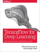
These metrics all emphasize different aspects of a classifier’s performance. They can also be useful in constructing some more sophisticated measurements of a binary classifier’s performance. For example, suppose that your binary classifier outputs class probabilities, and not just raw predictions. Then, there rises the question of choosing a cutoff. That is, at what probability of positive do you label the output as actually positive? The most common answer is 0.5, but by choosing higher or lower cutoffs, it is often possible to manually vary the balance between precision, recall, FPR, and TPR. These trade-offs are often represented graphically.
The receiver operator curve (ROC) plots the trade-off between the true positive rate and the false positive rate as the cutoff probability is varied (see Figure 5-1).
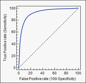
Figure 5-1. The receiver operator curve (ROC).
The area under curve (AUC) for the receiver operator curve (ROC-AUC) is a commonly measured metric. The ROC-AUC metric is useful since it provides a global picture of the binary classifier for all choices of cutoff. A perfect metric would have ROC-AUC 1.0 since the TPR would always be maximized. For comparison, a random classifier would have ROC-AUC 0.5. The ROC-AUC is often useful for imbalanced datasets, since the global view partially accounts for the imbalance in the dataset.
Multiclass Classification Metrics
Many common machine learning tasks require models to output classification labels that aren’t just binary. The ImageNet challenge (ILSVRC) required entrants to build models that would recognize which of a thousand potential object classes were in provided images, for example. Or in a simpler example, perhaps you want to predict tomorrow’s weather, where provided classes are “sunny,” “rainy,” and “cloudy.” How do you measure the performance of such a model?
The simplest method is to use a straightforward generalization of accuracy that measures the fraction of datapoints correctly labeled (Table 5-4).
| Metric | Definition |
|---|---|
Accuracy |
Num Correctly Labeled/Num Datapoints |
We note that there do exist multiclass generalizations of quantities like precision, recall, and ROC-AUC, and we encourage you to look into these definitions if interested. In practice, there’s a simpler visualization, the confusion matrix, which works well. For a multiclass problem with k classes, the confusion matrix is a k × k matrix. The (i, j)-th cell represents the number of datapoints labeled as class i with true label class j. Figure 5-2 illustrates a confusion matrix.
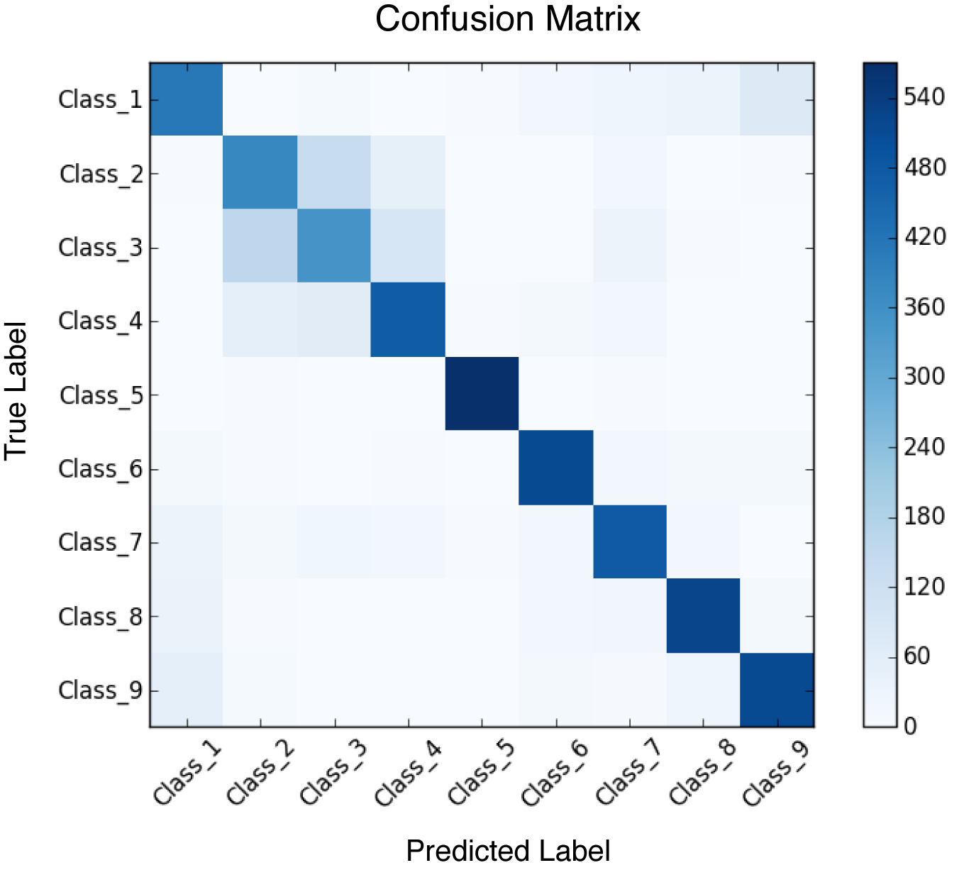
Figure 5-2. The confusion matrix for a 10-way classifier.
Don’t underestimate the power of the human eye to catch systematic failure patterns from simple visualizations! Looking at the confusion matrix can provide quick understanding that dozens of more complex multiclass metrics might miss.
Regression Metrics
You learned about regression metrics a few chapters ago. As a quick recap, the Pearson R2 and RMSE (root-mean-squared error) are good defaults.
We only briefly covered the mathematical definition of R2 previously, but will delve into it more now. Let represent predictions and represent labels. Let and represent the mean of the predicted values and the labels, respectively. Then the Pearson R (note the lack of square) is
This equation can be rewritten as
where cov represents the covariance and represents the standard deviation. Intuitively, the Pearson R measures the joint fluctuations of the predictions and labels from their means normalized by their respective ranges of fluctuations. If predictions and labels differ, these fluctuations will happen at different points and will tend to cancel, making R2 smaller. If predictions and labels tend to agree, the fluctuations will happen together and make R2 larger. We note that R2 is limited to a range between 0 and 1.
The RMSE measures the absolute quantity of the error between the predictions and the true quantities. It stands for root-mean-squared error, which is roughly analogous to the absolute value of the error between the true quantity and the predicted quantity. Mathematically, the RMSE is defined as follows (using the same notation as before):
Hyperparameter Optimization Algorithms
As we mentioned earlier in the chapter, hyperparameter optimization methods are learning algorithms for finding values of the hyperparameters that optimize the chosen metric on the validation set. In general, this objective function cannot be differentiated, so any optimization method must by necessity be a black box. In this section, we will show you some simple black-box learning algorithms for choosing hyperparameter values. We will use the Tox21 dataset from Chapter 4 as a case study to demonstrate these black-box optimization methods. The Tox21 dataset is small enough to make experimentation easy, but complex enough that hyperparameter optimization isn’t trivial.
We note before setting off that none of these black-box algorithms works perfectly. As you will soon see, in practice, much human input is required to optimize hyperparameters.
Can’t Hyperparameter Optimization Be Automated?
One of the long-running dreams of machine learning has been to automate the process of selecting model hyperparameters. Projects such as the “automated statistician” and others have sought to remove some of the drudgery from the hyperparameter selection process and make model construction more easily available to non-experts. However, in practice, there has typically been a steep cost in performance for the added convenience.
In recent years, there has been a surge of work focused on improving the algorithmic foundations of model tuning. Gaussian processes, evolutionary algorithms, and reinforcement learning have all been used to learn model hyperparameters and architectures with very limited human input. Recent work has shown that with large amounts of computing power, these algorithms can exceed expert performance in model tuning! But the overhead is severe, with dozens to hundreds of times greater computational power required.
For now, automatic model tuning is still not practical. All algorithms we cover in this section require significant manual tuning However, as hardware quality improves, we anticipate that hyperparameter learning will become increasingly automated. In the near term, we recommend strongly that all practitioners master the intricacies of hyperparameter tuning. A strong ability to hyperparameter tune is the skill that separates the expert from the novice.
Setting Up a Baseline
The first step in hyperparameter tuning is finding a baseline. A baseline is performance achievable by a robust (non–deep learning usually) algorithm. In general, random forests are a superb choice for setting baselines. As shown in Figure 5-3, random forests are an ensemble method that train many decision tree models on subsets of the input data and input features. These individual trees then vote on the outcome.
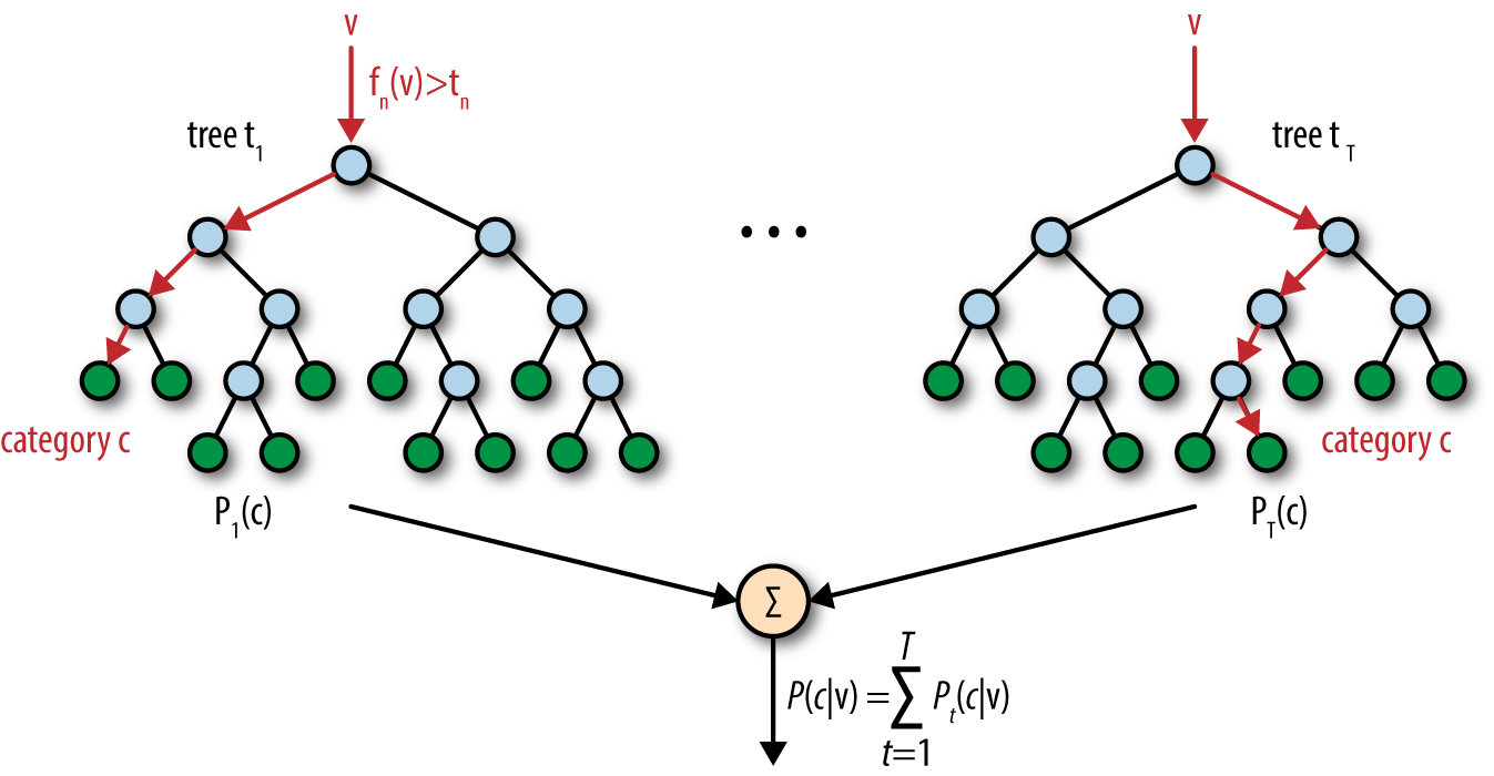
Figure 5-3. An illustration of a random forest. Here v is the input feature vector.
Random forests tend to be quite robust models. They are noise tolerant, and don’t worry about the scale of their input features. (Although we don’t have to worry about this for Tox21 since all our features are binary, in general deep networks are quite sensitive to their input range. It’s healthy to normalize or otherwise scale the input range for good performance. We will return to this point in later chapters.) They also tend to have strong generalization and don’t require much hyperparameter tuning to boot. For certain datasets, beating the performance of a random forest with a deep network can require considerable sophistication.
How can we create and train a random forest? Luckily for us, in Python, the scikit-learn library provides a high-quality implementation of a random forest. There are many tutorials and introductions to scikit-learn available, so we’ll just display the training and prediction code needed to build a Tox21 random forest model here (Example 5-1).
Example 5-1. Defining and training a random forest on the Tox21 dataset
fromsklearn.ensembleimportRandomForestClassifier# Generate tensorflow graphsklearn_model=RandomForestClassifier(class_weight="balanced",n_estimators=50)("About to fit model on training set.")sklearn_model.fit(train_X,train_y)train_y_pred=sklearn_model.predict(train_X)valid_y_pred=sklearn_model.predict(valid_X)test_y_pred=sklearn_model.predict(test_X)weighted_score=accuracy_score(train_y,train_y_pred,sample_weight=train_w)("Weighted train Classification Accuracy:%f"%weighted_score)weighted_score=accuracy_score(valid_y,valid_y_pred,sample_weight=valid_w)("Weighted valid Classification Accuracy:%f"%weighted_score)weighted_score=accuracy_score(test_y,test_y_pred,sample_weight=test_w)("Weighted test Classification Accuracy:%f"%weighted_score)
Here train_X, train_y, and so on are the Tox21 datasets defined in the previous chapter. Recall that all these quantities are NumPy arrays. n_estimators refers to the number of decision trees in our forest. Setting 50 or 100 trees often provides decent performance. Scikit-learn offers a simple object-oriented API with fit(X, y) and predict(X) methods. This model achieves the following accuracy with respect to our weighted accuracy metric:
Weighted train Classification Accuracy: 0.989845
Weighted valid Classification Accuracy: 0.681413
Recall that the fully connected network from Chapter 4 achieved performance:
Train Weighted Classification Accuracy: 0.742045
Valid Weighted Classification Accuracy: 0.648828
It looks like our baseline gets greater accuracy than our deep learning model! Time to roll up our sleeves and get to work.
Graduate Student Descent
The simplest method to try good hyperparameters is to simply try a number of different hyperparameter variants manually to see what works. This strategy can be surprisingly effective and educational. A deep learning practitioner needs to build up intuition about the structure of deep networks. Given the very weak state of theory, empirical work is the best way to learn how to build deep learning models. We highly recommend trying many variants of the fully connected model yourself. Be systematic; record your choices and results in a spreadsheet and systematically explore the space. Try to understand the effects of various hyperparameters. Which make network training proceed faster and which slower? What ranges of settings completely break learning? (These are quite easy to find, unfortunately.)
There are a few software engineering tricks that can make this search easier. Make a function whose arguments are the hyperparameter you wish to explore and have it print out the accuracy. Then trying new hyperparameter combinations requires only a single function call. Example 5-2 shows what this function signature would look like for our fully connected network from the Tox21 case study.
Example 5-2. A function mapping hyperparameters to different Tox21 fully connected networks
defeval_tox21_hyperparams(n_hidden=50,n_layers=1,learning_rate=.001,dropout_prob=0.5,n_epochs=45,batch_size=100,weight_positives=True):
Let’s walk through each of these hyperparameters. n_hidden controls the number of neurons in each hidden layer of the network. n_layers controls the number of hidden layers. learning_rate controls the learning rate used in gradient descent, and dropout_prob is the probability neurons are not dropped during training steps. n_epochs controls the number of passes through the total data and batch_size controls the number of datapoints in each batch.
weight_positives is the only new hyperparameter here. For unbalanced datasets, it can often be helpful to weight examples of both classes to have equal weight. For the Tox21 dataset, DeepChem provides weights for us to use. We simply multiply the per-example cross-entropy terms by the weights to perform this weighting (Example 5-3).
Example 5-3. Weighting positive samples for Tox21
entropy=tf.nn.sigmoid_cross_entropy_with_logits(logits=y_logit,labels=y_expand)# Multiply by weightsifweight_positives:w_expand=tf.expand_dims(w,1)entropy=w_expand*entropy
Why is the method of picking hyperparameter values called graduate student descent? Machine learning, until recently, has been a primarily academic field. The tried-and-true method for designing a new machine learning algorithm has been describing the method desired to a new graduate student, and asking them to work out the details. This process is a bit of a rite of passage, and often requires the student to painfully try many design alternatives. On the whole, this is a very educational experience, since the only way to gain design aesthetic is to build up a memory of settings that work and don’t work.
Grid Search
After having tried a few manual settings for hyperparameters, the process will begin to feel very tedious. Experienced programmers will be tempted to simply write a for loop that iterates over the choices of hyperparameters desired. This process is more or less the grid-search method. For each hyperparameter, pick a list of values that might be good hyperparameters. Write a nested for loop that tries all combinations of these values to find their validation accuracies, and keep track of the best performers.
There is one subtlety in the process, however. Deep networks can be fairly sensitive to the choice of random seed used to initialize the network. For this reason, it’s worth repeating each choice of hyperparameter settings multiple times and averaging the results to damp the variance.
The code to do this is straightforward, as Example 5-4 shows.
Example 5-4. Performing grid search on Tox21 fully connected network hyperparameters
scores={}n_reps=3hidden_sizes=[50]epochs=[10]dropouts=[.5,1.0]num_layers=[1,2]forrepinrange(n_reps):forn_epochsinepochs:forhidden_sizeinhidden_sizes:fordropoutindropouts:forn_layersinnum_layers:score=eval_tox21_hyperparams(n_hidden=hidden_size,n_epochs=n_epochs,dropout_prob=dropout,n_layers=n_layers)if(hidden_size,n_epochs,dropout,n_layers)notinscores:scores[(hidden_size,n_epochs,dropout,n_layers)]=[]scores[(hidden_size,n_epochs,dropout,n_layers)].append(score)("All Scores")(scores)avg_scores={}forparams,param_scoresinscores.iteritems():avg_scores[params]=np.mean(np.array(param_scores))("Scores Averaged over%drepetitions"%n_reps)
Random Hyperparameter Search
For experienced practitioners, it will often be very tempting to reuse magical hyperparameter settings or search grids that worked in previous applications. These settings can be valuable, but they can also lead us astray. Each machine learning problem is slightly different, and the optimal settings might lie in a region of parameter space we haven’t previously considered. For that reason, it’s often worthwhile to try random settings for hyperparameters (where the random values are chosen from a reasonable range).
There’s also a deeper reason to try random searches. In higher-dimensional spaces, regular grids can miss a lot of information, especially if the spacing between grid points isn’t great. Selecting random choices for grid points can help us from falling into the trap of loose grids. Figure 5-4 illustrates this fact.
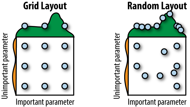
Figure 5-4. An illustration of why random hyperparameter search can be superior to grid search.
How can we implement random hyperparameter search in software? A neat software trick is to sample the random values desired up front and store them in a list. Then, random hyperparameter search simply turns into grid search over these randomly sampled lists. Here’s an example. For learning rates, it’s often useful to try a wide range from .1 to .000001 or so. Example 5-5 uses NumPy to sample some random learning rates.
Example 5-5. Sampling random learning rates
n_rates=5learning_rates=10**(-np.random.uniform(low=1,high=6,size=n_rates))
We use a mathematical trick here. Note that .1 = 10–1 and .000001 = 10–6. Sampling real-valued numbers between ranges like 1 and 6 is easy with np.random.uniform. We can raise these sampled values to a power to recover our learning rates. Then learning_rates holds a list of values that we can feed into our grid search code from the previous section.
Challenge for the Reader
In this chapter, we’ve only covered the basics of hyperparameter tuning, but the tools covered are quite powerful. As a challenge, try tuning the fully connected deep network to achieve validation performance higher than that of the random forest. This might require a bit of work, but it’s well worth the experience.
Review
In this chapter, we covered the basics of hyperparameter optimization, the process of selecting values for model parameters that can’t be learned automatically on the training data. In particular, we introduced random and grid hyperparameter search and demonstrated the use of such code for optimizing models on the Tox21 dataset introduced in the last chapter.
In Chapter 6, we will return to our survey of deep architectures and introduce you to convolutional neural networks, one of the fundamental building blocks of modern deep architectures.