
Chapter 5. Paint
So far, we have explored various ways in which we can train a model to generate new samples, given only a training set of data we wish to imitate. We’ve applied this to several datasets and seen how in each case, VAEs and GANs are able to learn a mapping between an underlying latent space and the original pixel space. By sampling from a distribution in the latent space, we can use the generative model to map this vector to a novel image in the pixel space.
Notice that all of the examples we have seen so far produce novel observations from scratch—that is, there is no input apart from the random latent vector sampled from the latent space that is used to generate the images.
A different application of generative models is in the field of style transfer. Here, our aim is to build a model that can transform an input base image in order to give the impression that it comes from the same collection as a given set of style images. This technique has clear commercial applications and is now being used in computer graphics software, computer game design, and mobile phone applications. Some examples of this are shown in Figure 5-1.
With style transfer, our aim isn’t to model the underlying distribution of the style images, but instead to extract only the stylistic components from these images and embed these into the base image. We clearly cannot just merge the style images with the base image through interpolation, as the content of the style images would show through and the colors would become muddy and blurred. Moreover, it may be the style image set as a whole rather than one single image that captures the artist’s style, so we need to find a way to allow the model to learn about style across a whole collection of images. We want to give the impression that the artist has used the base image as a guide to produce an original piece of artwork, complete with the same stylistic flair as other works in their collection.

Figure 5-1. Style transfer examples1
In this chapter you’ll learn how to build two different kinds of style transfer model (CycleGAN and Neural Style Transfer) and apply the techniques to your own photos and artwork.
We’ll start by visiting a fruit and vegetable shop where all is not as it seems…
Apples and Organges
Granny Smith and Florida own a greengrocers together. To ensure the shop is run as efficiently as possible, they each look after different areas—specifically, Granny Smith takes great pride in her apple selection and Florida spends hours ensuring the oranges are perfectly arranged.
Both are so convinced that they have the better fruit display that they agree to a deal: the profits from the sales of apples will go entirely to Granny Smith and the profits from the sales of oranges will go entirely to Florida.
Unfortunately, neither Granny Smith nor Florida plans on making this a fair contest. When Florida isn’t looking, Granny Smith sneaks into the orange section and starts painting the oranges red to look like apples! Florida has exactly the same plan, and tries to make Granny Smith’s apples more orange-like with a suitably colored spray when her back is turned.
When customers bring their fruit to the self-checkout tills, they sometimes erroneously select the wrong option on the machine. Customers who took apples sometimes put them through as oranges due to Florida’s fluorescent spray, and customers who took oranges wrongly pay for apples due to their clever disguise, courtesy of Granny Smith.
At the end of the day, the profits for each fruit are summed and split accordingly—Granny Smith loses money every time one of her apples is sold as an orange, and Florida loses every time one of her oranges is sold as an apple.
After closing time, both of the disgruntled greengrocers do their best to clean up their own fruit stocks. However, instead of trying to undo the other’s mischievous adjustments, they both simply apply their own tampering process to their own fruit, to try to make it appear as it did before it was sabotaged. It’s important that they get this right, because if the fruit doesn’t look right, they won’t be able to sell it the next day and will again lose profits.
To ensure consistency over time, they also test their techniques out on their own fruit. Florida checks that if she sprays her oranges orange, they’ll look exactly as they did originally. Granny Smith tests her apple painting skills on her apples for the same reason. If they find that there are obvious discrepancies, they’ll have to spend their hard-earned profits on learning better techniques.
The overall process is shown in Figure 5-2.
At first, customers are inclined to make somewhat random selections at the newly installed self-checkout tills because of their inexperience with the machines. However, over time they become more adept at using the technology, and learn how to identify which fruit has been tampered with.
This forces Granny Smith and Florida to improve at sabotaging each other’s fruit, while also always ensuring that they are still able to use the same process to clean up their own fruit after it has been altered. Moreover, they must also make sure that the technique they use doesn’t affect the appearance of their own fruit.

Figure 5-2. Diagram of the greengrocers’ tampering, restoration, and testing process
After many days and weeks of this ridiculous game, they realize something amazing has happened. Customers are thoroughly confused and now can’t tell the difference between real and fake apples and real and fake oranges. Figure 5-3 shows the state of the fruit after tampering and restoration, as well as after testing.

Figure 5-3. Examples of the oranges and apples in the greengrocers’ store
CycleGAN
The preceding story is an allegory for a key development in generative modeling and, in particular, style transfer: the cycle-consistent adversarial network, or CycleGAN. The original paper represented a significant step forward in the field of style transfer as it showed how it was possible to train a model that could copy the style from a reference set of images onto a different image, without a training set of paired examples.2
Previous style transfer models, such as pix2pix,3 required each image in the training set to exist in both the source and target domain. While it is possible to manufacture this kind of dataset for some style problem settings (e.g., black and white to color photos, maps to satellite images), for others it is impossible. For example, we do not have original photographs of the pond where Monet painted his Water Lilies series, nor do we have a Picasso painting of the Empire State Building. It would also take enormous effort to arrange photos of horses and zebras standing in identical positions.
The CycleGAN paper was released only a few months after the pix2pix paper and shows how it is possible to train a model to tackle problems where we do not have pairs of images in the source and target domains. Figure 5-4 shows the difference between the paired and unpaired datasets of pix2pix and CycleGAN, respectively.

Figure 5-4. pix2pix dataset and domain mapping example
While pix2pix only works in one direction (from source to target), CycleGAN trains the model in both directions simultaneously, so that the model learns to translate images from target to source as well as source to target. This is a consequence of the model architecture, so you get the reverse direction for free.
Let’s now see how we can build a CycleGAN model in Keras. To begin with, we shall be using the apples and oranges example from earlier to walk through each part of the CycleGAN and experiment with the architecture. We’ll then apply the same technique to build a model that can apply a given artist’s style to a photo of your choice.
Your First CycleGAN
Much of the following code has been inspired by and adapted from the amazing Keras-GAN repository maintained by Erik Linder-Norén. This is an excellent resource for many Keras examples of important GANs from the literature.
To begin, you’ll first need to download the data that we’ll be using to train the CycleGAN. From inside the folder where you cloned the book’s repository, run the following command:
bash ./scripts/download_cyclegan_data.sh apple2orange
This will download the dataset of images of apples and oranges that we will be using. The data is split into four folders: trainA and testA contain images of apples and trainB and testB contain images of oranges. Thus domain A is the space of apple images and domain B is the space of orange images. Our goal is to train a model using the train datasets to convert images from domain A into domain B and vice versa. We will test our model using the test datasets.
Overview
A CycleGAN is actually composed of four models, two generators and two discriminators. The first generator, G_AB, converts images from domain A into domain B. The second generator, G_BA, converts images from domain B into domain A.
As we do not have paired images on which to train our generators, we also need to train two discriminators that will determine if the images produced by the generators are convincing. The first discriminator, d_A, is trained to be able to identify the difference between real images from domain A and fake images that have been produced by generator G_BA. Conversely, discriminator d_B is trained to be able to identify the difference between real images from domain B and fake images that have been produced by generator G_AB. The relationship between the four models is shown in Figure 5-5.

Figure 5-5. Diagram of the four CycleGAN models4
Running the notebook 05_01_cyclegan_train.ipynb in the book repository will start training the CycleGAN. As in previous chapters, you can instantiate a CycleGAN object in the notebook, as shown in Example 5-1, and play around with the parameters to see how it affects the model.
Example 5-1. Defining the CycleGAN
gan=CycleGAN(input_dim=(128,128,3),learning_rate=0.0002,lambda_validation=1,lambda_reconstr=10,lambda_id=2,generator_type='u-net',gen_n_filters=32,disc_n_filters=32)
Let’s first take a look at the architecture of the generators. Typically, CycleGAN generators take one of two forms: U-Net or ResNet (residual network). In their earlier pix2pix paper,5 the authors used a U-Net architecture, but they switched to a ResNet architecture for CycleGAN. We’ll be building both architectures in this chapter, starting with U-Net.6
The Generators (U-Net)
Figure 5-6 shows the architecture of the U-Net we will be using—no prizes for guessing why it’s called a U-Net!7

Figure 5-6. The U-Net architecture diagram
In a similar manner to a variational autoencoder, a U-Net consists of two halves: the downsampling half, where input images are compressed spatially but expanded channel-wise, and an upsampling half, where representations are expanded spatially while the number of channels is reduced.
However, unlike in a VAE, there are also skip connections between equivalently shaped layers in the upsampling and downsampling parts of the network. A VAE is linear; data flows through the network from input to the output, one layer after another. A U-Net is different, because it contains skip connections that allow information to shortcut parts of the network and flow through to later layers.
The intuition here is that with each subsequent layer in the downsampling part of the network, the model increasingly captures the what of the images and loses information on the where. At the apex of the U, the feature maps will have learned a contextual understanding of what is in the image, with little understanding of where it is located. For predictive classification models, this is all we require, so we could connect this to a final Dense layer to output the probability of a particular class being present in the image. However, for the original U-Net application (image segmentation) and also for style transfer, it is critical that when we upsample back to the original image size, we pass back into each layer the spatial information that was lost during downsampling. This is exactly why we need the skip connections. They allow the network to blend high-level abstract information captured during the downsampling process (i.e., the image style) with the specific spatial information that is being fed back in from previous layers in the network (i.e., the image content).
To build in the skip connections, we will need to introduce a new type of layer: `Concatenate`.
The generator also contains another new layer type, InstanceNormalization.
We now have everything we need to build a U-Net generator in Keras, as shown in Example 5-2.
Example 5-2. Building the U-Net generator
defbuild_generator_unet(self):defdownsample(layer_input,filters,f_size=4):d=Conv2D(filters,kernel_size=f_size,strides=2,padding='same')(layer_input)d=InstanceNormalization(axis=-1,center=False,scale=False)(d)d=Activation('relu')(d)returnddefupsample(layer_input,skip_input,filters,f_size=4,dropout_rate=0):u=UpSampling2D(size=2)(layer_input)u=Conv2D(filters,kernel_size=f_size,strides=1,padding='same')(u)u=InstanceNormalization(axis=-1,center=False,scale=False)(u)u=Activation('relu')(u)ifdropout_rate:u=Dropout(dropout_rate)(u)u=Concatenate()([u,skip_input])returnu# Image inputimg=Input(shape=self.img_shape)# Downsamplingd1=downsample(img,self.gen_n_filters)d2=downsample(d1,self.gen_n_filters*2)d3=downsample(d2,self.gen_n_filters*4)d4=downsample(d3,self.gen_n_filters*8)# Upsamplingu1=upsample(d4,d3,self.gen_n_filters*4)u2=upsample(u1,d2,self.gen_n_filters*2)u3=upsample(u2,d1,self.gen_n_filters)u4=UpSampling2D(size=2)(u3)output=Conv2D(self.channels,kernel_size=4,strides=1,padding='same',activation='tanh')(u4)returnModel(img,output)
The Discriminators
The discriminators that we have seen so far have output a single number: the predicted probability that the input image is “real.” The discriminators in the CycleGAN that we will be building output an 8 × 8 single-channel tensor rather than a single number.
The reason for this is that the CycleGAN inherits its discriminator architecture from a model known as a PatchGAN, where the discriminator divides the image into square overlapping “patches” and guesses if each patch is real or fake, rather than predicting for the image as a whole. Therefore the output of the discriminator is a tensor that contains the predicted probability for each patch, rather than just a single number.
Note that the patches are predicted simultaneously as we pass an image through the network—we do not divide up the image manually and pass each patch through the network one by one. The division of the image into patches arises naturally as a result of the discriminator’s convolutional architecture.
The benefit of using a PatchGAN discriminator is that the loss function can then measure how good the discriminator is at distinguishing images based on their style rather than their content. Since each individual element of the discriminator prediction is based only on a small square of the image, it must use the style of the patch, rather than its content, to make its decision. This is exactly what we require; we would rather our discriminator is good at identifying when two images differ in style than content.
The Keras code to build the discriminators is provided in Example 5-3.
Example 5-3. Building the discriminators
defbuild_discriminator(self):defconv4(layer_input,filters,stride=2,norm=True):y=Conv2D(filters,kernel_size=4,strides=stride,padding='same')(layer_input)ifnorm:y=InstanceNormalization(axis=-1,center=False,scale=False)(y)y=LeakyReLU(0.2)(y)returnyimg=Input(shape=self.img_shape)y=conv4(img,self.disc_n_filters,stride=2,norm=False)y=conv4(y,self.disc_n_filters*2,stride=2)y=conv4(y,self.disc_n_filters*4,stride=2)y=conv4(y,self.disc_n_filters*8,stride=1)output=Conv2D(1,kernel_size=4,strides=1,padding='same')(y)returnModel(img,output)

A CycleGAN discriminator is a series of convolutional layers, all with instance normalization (except the first layer).

The final layer is a convolutional layer with only one filter and no activation.
Compiling the CycleGAN
To recap, we aim to build a set of models that can convert images that are in domain A (e.g., images of apples) to domain B (e.g., images of oranges) and vice versa. We therefore need to compile four distinct models, two generators and two discriminators, as follows:
g_AB-
Learns to convert an image from domain A to domain B.
g_BA-
Learns to convert an image from domain B to domain A.
d_A-
Learns the difference between real images from domain A and fake images generated by
g_BA. d_B-
Learns the difference between real images from domain B and fake images generated by
g_AB.
We can compile the two discriminators directly, as we have the inputs (images from each domain) and outputs (binary responses: 1 if the image was from the domain or 0 if it was a generated fake). This is shown in Example 5-4.
Example 5-4. Compiling the discriminator
self.d_A=self.build_discriminator()self.d_B=self.build_discriminator()self.d_A.compile(loss='mse',optimizer=Adam(self.learning_rate,0.5),metrics=['accuracy'])self.d_B.compile(loss='mse',optimizer=Adam(self.learning_rate,0.5),metrics=['accuracy'])
However, we cannot compile the generators directly, as we do not have paired images in our dataset. Instead, we judge the generators simultaneously on three criteria:
-
Validity. Do the images produced by each generator fool the relevant discriminator? (For example, does output from
g_BAfoold_Aand does output fromg_ABfoold_B?) -
Reconstruction. If we apply the two generators one after the other (in both directions), do we return to the original image? The CycleGAN gets its name from this cyclic reconstruction criterion.
-
Identity. If we apply each generator to images from its own target domain, does the image remain unchanged?
Example 5-5 shows how we can compile a model to enforce these three criteria (the numeric markers in the code correspond to the preceding list).
Example 5-5. Building the combined model to train the generators
self.g_AB=self.build_generator_unet()self.g_BA=self.build_generator_unet()self.d_A.trainable=Falseself.d_B.trainable=Falseimg_A=Input(shape=self.img_shape)img_B=Input(shape=self.img_shape)fake_A=self.g_BA(img_B)fake_B=self.g_AB(img_A)valid_A=self.d_A(fake_A)valid_B=self.d_B(fake_B)reconstr_A=self.g_BA(fake_B)reconstr_B=self.g_AB(fake_A)img_A_id=self.g_BA(img_A)img_B_id=self.g_AB(img_B)self.combined=Model(inputs=[img_A,img_B],outputs=[valid_A,valid_B,reconstr_A,reconstr_B,img_A_id,img_B_id])self.combined.compile(loss=['mse','mse','mae','mae','mae','mae'],loss_weights=[self.lambda_validation,self.lambda_validation,self.lambda_reconstr,self.lambda_reconstr,self.lambda_id,self.lambda_id],optimizer=optimizer)
The combined model accepts a batch of images from each domain as input and provides three outputs (to match the three criteria) for each domain—so, six outputs in total. Notice how we freeze the weights in the discriminator, as is typical with GANs, so that the combined model only trains the generator weights, even though the discriminator is involved in the model.
The overall loss is the weighted sum of the loss for each criterion. Mean squared error is used for the validity criterion—checking the output from the discriminator against the real (1) or fake (0) response—and mean absolute error is used for the image-to-image-based criteria (reconstruction and identity).
Training the CycleGAN
With our discriminators and combined model compiled, we can now train our models. This follows the standard GAN practice of alternating the training of the discriminators with the training of the generators (through the combined model).
In Keras, the code in Example 5-6 describes the training loop.
Example 5-6. Training the CycleGAN
batch_size=1patch=int(self.img_rows/2**4)self.disc_patch=(patch,patch,1)valid=np.ones((batch_size,)+self.disc_patch)fake=np.zeros((batch_size,)+self.disc_patch)forepochinrange(self.epoch,epochs):forbatch_i,(imgs_A,imgs_B)inenumerate(data_loader.load_batch(batch_size)):fake_B=self.g_AB.predict(imgs_A)fake_A=self.g_BA.predict(imgs_B)dA_loss_real=self.d_A.train_on_batch(imgs_A,valid)dA_loss_fake=self.d_A.train_on_batch(fake_A,fake)dA_loss=0.5*np.add(dA_loss_real,dA_loss_fake)dB_loss_real=self.d_B.train_on_batch(imgs_B,valid)dB_loss_fake=self.d_B.train_on_batch(fake_B,fake)dB_loss=0.5*np.add(dB_loss_real,dB_loss_fake)d_loss=0.5*np.add(dA_loss,dB_loss)g_loss=self.combined.train_on_batch([imgs_A,imgs_B],[valid,valid,imgs_A,imgs_B,imgs_A,imgs_B])
We use a response of 1 for real images and 0 for generated images. Notice how there is one response per patch, as we are using a PatchGAN discriminator.
To train the discriminators, we first use the respective generator to create a batch of fake images, then we train each discriminator on this fake set and a batch of real images. Typically, for a CycleGAN the batch size is 1 (a single image).

The generators are trained together in one step, through the combined model compiled earlier. See how the six outputs match to the six loss functions defined earlier during compilation.
Analysis of the CycleGAN
Let’s see how the CycleGAN performs on our simple dataset of apples and oranges and observe how changing the weighting parameters in the loss function can have dramatic effects on the results.
We have already seen an example of the output from the CycleGAN model in Figure 5-3. Now that you are familiar with the CycleGAN architecture, you might recognize that this image represents the three criteria through which the combined model is judged: validity, reconstruction, and identity.
Let’s relabel this image with the appropriate functions from the codebase, so that we can see this more explicitly (Figure 5-8).
We can see that the training of the network has been successful, because each generator is visibly altering the input picture to look more like a valid image from the opposite domain. Moreover, when the generators are applied one after the other, the difference between the input image and the reconstructed image is minimal. Finally, when each generator is applied to an image from its own input domain, the image doesn’t change significantly.

Figure 5-8. Outputs from the combined model used to calculated the overall loss function
In the original CycleGAN paper, the identity loss was included as an optional addition to the necessary reconstruction loss and validity loss. To demonstrate the importance of the identity term in the loss function, let’s see what happens if we remove it, by setting the identity loss weighting parameter to zero in the loss function (Figure 5-9).

Figure 5-9. Output from the CycleGAN when the identity loss weighting is set to zero
The CycleGAN has still managed to translate the oranges into apples but the color of the tray holding the oranges has flipped from black to white, as there is now no identity loss term to prevent this shift in background colors. The identity term helps regulate the generator to ensure that it only adjust parts of the image that are necessary to complete the transformation and no more.
This highlights the importance of ensuring the weightings of the three loss functions are well balanced—too little identity loss and the color shift problem appears; too much identity loss and the CycleGAN isn’t sufficiently incentivized to change the input to look like an image from the opposite domain.
Creating a CycleGAN to Paint Like Monet
Now that we have explored the fundamental structure of a CycleGAN, we can turn our attention to more interesting and impressive applications of the technique.
In the original CycleGAN paper, one of the standout achievements was the ability for the model to learn how to convert a given photo into a painting in the style of a particular artist. As this is a CycleGAN, the model is also able to translate the other way, converting an artist’s paintings into realistic-looking photographs.
To download the Monet-to-photo dataset, run the following command from inside the book repository:
bash ./scripts/download_cyclegan_data.sh monet2photo
This time we will use the parameter set shown in Example 5-7 to build the model:
Example 5-7. Defining the Monet CycleGAN
gan=CycleGAN(input_dim=(256,256,3),learning_rate=0.0002,lambda_validation=1,lambda_reconstr=10,lambda_id=5,generator_type='resnet',gen_n_filters=32,disc_n_filters=64)
The Generators (ResNet)
In this example, we shall introduce a new type of generator architecture: a residual network, or ResNet.10 The ResNet architecture is similar to a U-Net in that it allows information from previous layers in the network to skip ahead one or more layers. However, rather than creating a U shape by connecting layers from the downsampling part of the network to corresponding upsampling layers, a ResNet is built of residual blocks stacked on top of each other, where each block contains a skip connection that sums the input and output of the block, before passing this on to the next layer. A single residual block is shown in Figure 5-10.

Figure 5-10. A single residual block
In our CycleGAN, the “weight layers” in the diagram are convolutional layers with instance normalization. In Keras, a residual block can be coded as shown in Example 5-8.
Example 5-8. A residual block in Keras
fromkeras.layers.mergeimportadddefresidual(layer_input,filters):shortcut=layer_inputy=Conv2D(filters,kernel_size=(3,3),strides=1,padding='same')(layer_input)y=InstanceNormalization(axis=-1,center=False,scale=False)(y)y=Activation('relu')(y)y=Conv2D(filters,kernel_size=(3,3),strides=1,padding='same')(y)y=InstanceNormalization(axis=-1,center=False,scale=False)(y)returnadd([shortcut,y])
On either side of the residual blocks, our ResNet generator also contains downsampling and upsampling layers. The overall architecture of the ResNet is shown in Figure 5-11.

Figure 5-11. A ResNet generator
It has been shown that ResNet architectures can be trained to hundreds and even thousands of layers deep and not suffer from the vanishing gradient problem, where the gradients at early layers are tiny and therefore train very slowly. This is due to the fact that the error gradients can backpropagate freely through the network through the skip connections that are part of the residual blocks. Furthermore, it is believed that adding additional layers never results in a drop in model accuracy, as the skip connections ensure that it is always possible to pass through the identity mapping from the previous layer, if no further informative features can be extracted.
Analysis of the CycleGAN
In the original CycleGAN paper, the model was trained for 200 epochs to achieve state-of-the-art results for artist-to-photograph style transfer. In Figure 5-12 we show the output from each generator at various stages of the early training process, to show the progression as the model begins to learn how to convert Monet paintings into photographs and vice versa.
In the top row, we can see that gradually the distinctive colors and brushstrokes used by Monet are transformed into the more natural colors and smooth edges that would be expected in a photograph. Similarly, the reverse is happening in the bottom row, as the generator learns how to convert a photograph into a scene that Monet might have painted himself.

Figure 5-12. Output at various stages of the training process
Figure 5-13 shows some of the results from the original paper achieved by the model after it was trained for 200 epochs.

Figure 5-13. Output after 200 epochs of training11
Neural Style Transfer
So far, we have seen how a CycleGAN can transpose images between two domains, where the images in the training set are not necessarily paired. Now we shall look at a different application of style transfer, where we do not have a training set at all, but instead wish to transfer the style of one single image onto another, as shown in Figure 5-14. This is known as neural style transfer.12
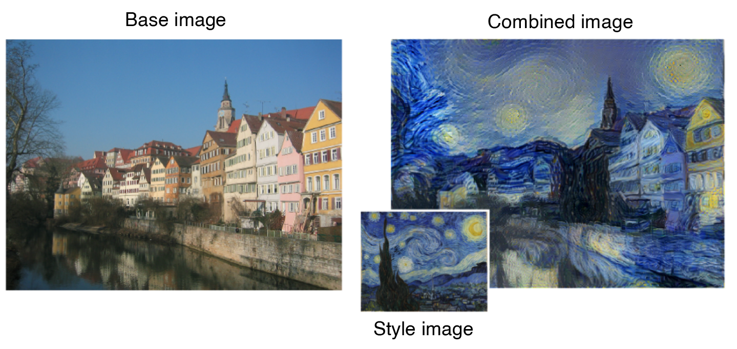
Figure 5-14. An example of neural style transfer13
The idea works on the premise that we want to minimize a loss function that is a weighted sum of three distinct parts:
- Content loss
-
We would like the combined image to contain the same content as the base image.
- Style loss
-
We would like the combined image to have the same general style as the style image.
- Total variance loss
-
We would like the combined image to appear smooth rather than pixelated.
We minimize this loss via gradient descent—that is, we update each pixel value by an amount proportional to the negative gradient of the loss function, over many iterations. This way, the loss gradually decreases with each iteration and we end up with an image that merges the content of one image with the style of another.
Optimizing the generated output via gradient descent is different to how we have tackled generative modeling problems thus far. Previously we have trained a deep neural network such as a VAE or GAN by backpropagating the error through the entire network to learn from a training set of data and generalize the information learned to generate new images. Here, we cannot take this approach as we only have two images to work with, the base image and the style image. However, as we shall see, we can still make use of a pretrained deep neural network to provide vital information about each image inside the loss functions.
We’ll start by defining the three individual loss functions, as they are the core of the neural style transfer engine.
Content Loss
The content loss measures how different two images are in terms of the subject matter and overall placement of their content. Two images that contain similar-looking scenes (e.g., a photo of a row of buildings and another photo of the same buildings taken in different light from a different angle) should have a smaller loss than two images that contain completely different scenes. Simply comparing the pixel values of the two images won’t do, because even in two distinct images of the same scene, we wouldn’t expect individual pixel values to be similar. We don’t really want the content loss to care about the values of individual pixels; we’d rather that it scores images based on the presence and approximate position of higher-level features such as buildings, sky, or river.
We’ve seen this concept before. It’s the whole premise behind deep learning—a neural network trained to recognize the content of an image naturally learns higher-level features at deeper layers of the network by combining simpler features from previous layers. Therefore, what we need is a deep neural network that has already been successfully trained to identify the content of an image, so that we can tap into a deep layer of the network to extract the high-level features of a given input image. If we measure the mean squared error between this output for the base image and the current combined image, we have our content loss function!
The pretrained network that we shall be using is called VGG19. This is a 19-layer convolutional neural network that has been trained to classify images into one thousand object categories on more than one million images from the ImageNet dataset. A diagram of the network is shown in Figure 5-15.

Figure 5-15. The VGG19 model
Example 5-9 is a code snippet that calculates the content loss between two images, adapted from the neural style transfer example in the official Keras repository. If you want to re-create this technique and experiment with the parameters, I suggest working from this repository as a starting point.
Example 5-9. The content loss function
fromkeras.applicationsimportvgg19fromkerasimportbackendasKbase_image_path='/path_to_images/base_image.jpg'style_reference_image_path='/path_to_images/styled_image.jpg'content_weight=0.01base_image=K.variable(preprocess_image(base_image_path))style_reference_image=K.variable(preprocess_image(style_reference_image_path))combination_image=K.placeholder((1,img_nrows,img_ncols,3))input_tensor=K.concatenate([base_image,style_reference_image,combination_image],axis=0)model=vgg19.VGG19(input_tensor=input_tensor,weights='imagenet',include_top=False)outputs_dict=dict([(layer.name,layer.output)forlayerinmodel.layers])layer_features=outputs_dict['block5_conv2']base_image_features=layer_features[0,:,:,:]combination_features=layer_features[2,:,:,:]defcontent_loss(content,gen):returnK.sum(K.square(gen-content))content_loss=content_weight*content_loss(base_image_features,combination_features)
The Keras library contains a pretrained VGG19 model that can be imported.
We define two Keras variables to hold the base image and style image and a placeholder that will contain the generated combined image.
The input tensor to the VGG19 model is a concatenation of the three images.

Here we create an instance of the VGG19 model, specifying the input tensor and the weights that we would like to preload. The
include_top = Falseparameter specifies that we do not need to load the weights for the final dense layers of the networks that result in the classification of the image. This is because we are only interested in the preceding convolutional layers, which capture the high-level features of an input image, not the actual probabilities that the original model was trained to output.
The layer that we use to calculate the content loss is the second convolutional layer of the fifth block. Choosing a layer at a shallower or deeper point in the network affects how the loss function defines “content” and therefore alters the properties of the generated combined image.

Here we extract the base image features and combined image features from the input tensor that has been fed through the VGG19 network.

The content loss is the sum of squares distance between the outputs of the chosen layer for both images, multiplied by a weighting parameter.
Style Loss
Style loss is slightly more difficult to quantify—how can we measure the similarity in style between two images?
The solution given in the neural style transfer paper is based on the idea that images that are similar in style typically have the same pattern of correlation between feature maps in a given layer. We can see this more clearly with an example.
Suppose in the VGG19 network we have some layer where one channel has learned to identify parts of the image that are colored green, another channel has learned to identify spikiness, and another has learned to identify parts of the image that are brown.
The output from these channels (feature maps) for three inputs is shown in Figure 5-16.

Figure 5-16. The output from three channels (feature maps) for three given input images—the darker orange colors represent larger values
We can see that A and B are similar in style—both are grassy. Image C is slightly different in style to images A and B. If we look at the feature maps, we can see that the green and spikiness channels often fire strongly together at the same spatial point in images A and B, but not in image C. Conversely, the brown and spikiness channels are often activated together at the same point in image C, but not in images A and B. To numerically measure how much two feature maps are jointly activated together, we can flatten them and calculate the dot product.14 If the resulting value is high, the feature maps are highly correlated; if the value is low, the feature maps are not correlated.
We can define a matrix that contains the dot product between all possible pairs of features in the layer. This is called a Gram matrix. Figure 5-17 shows the Gram matrices for the three features, for each of the images.

Figure 5-17. Parts of the Gram matrices for the three images—the darker blue colors represent larger values
It is clear that images A and B, which are similar in style, have similar Gram matrices for this layer. Even though their content may be very different, the Gram matrix—a measure of correlation between all pairs of features in the layer—is similar.
Therefore to calculate the style loss, all we need to do is calculate the Gram matrix (GM) for a set of layers throughout the network for both the base image and the combined image and compare their similarity using sum of squared errors. Algebraically, the style loss between the base image (S) and the generated image (G) for a given layer (l) of size Ml (height x width) with Nl channels can be written as follows:
Notice how this is scaled to account for the number of channels (Nl) and size of the layer (Ml). This is because we calculate the overall style loss as a weighted sum across several layers, all of which have different sizes. The total style loss is then calculated as follows:
In Keras, the style loss calculations can be coded as shown in Example 5-10.15
Example 5-10. The style loss function
style_loss=0.0defgram_matrix(x):features=K.batch_flatten(K.permute_dimensions(x,(2,0,1)))gram=K.dot(features,K.transpose(features))returngramdefstyle_loss(style,combination):S=gram_matrix(style)C=gram_matrix(combination)channels=3size=img_nrows*img_ncolsreturnK.sum(K.square(S-C))/(4.0*(channels**2)*(size**2))feature_layers=['block1_conv1','block2_conv1','block3_conv1','block4_conv1','block5_conv1']forlayer_nameinfeature_layers:layer_features=outputs_dict[layer_name]style_reference_features=layer_features[1,:,:,:]combination_features=layer_features[2,:,:,:]sl=style_loss(style_reference_features,combination_features)style_loss+=(style_weight/len(feature_layers))*sl
The style loss is calculated over five layers—the first convolutional layer in each of the five blocks of the VGG19 model.
Here we extract the style image features and combined image features from the input tensor that has been fed through the VGG19 network.
The style loss is scaled by a weighting parameter and the number of layers that it is calculated over.
Total Variance Loss
The total variance loss is simply a measure of noise in the combined image. To judge how noisy an image is, we can shift it one pixel to the right and calculate the sum of the squared difference between the translated and original images. For balance, we can also do the same procedure but shift the image one pixel down. The sum of these two terms is the total variance loss.
Example 5-11 shows how we can code this in Keras.16
Example 5-11. The variance loss function
deftotal_variation_loss(x):a=K.square(x[:,:img_nrows-1,:img_ncols-1,:]-x[:,1:,:img_ncols-1,:])b=K.square(x[:,:img_nrows-1,:img_ncols-1,:]-x[:,:img_nrows-1,1:,:])returnK.sum(K.pow(a+b,1.25))tv_loss=total_variation_weight*total_variation_loss(combination_image)loss=content_loss+style_loss+tv_loss
The squared difference between the image and the same image shifted one pixel down.
The squared difference between the image and the same image shifted one pixel to the right.
The total variance loss is scaled by a weighting parameter.
The overall loss is the sum of the content, style, and total variance losses.
Running the Neural Style Transfer
The learning process involves running gradient descent to minimize this loss function, with respect to the pixels in the combined image. The full code for this is included in the, neural_style_transfer.py script included as part of the official Keras repository. Example 5-12 is a code snippet showing the training loop.
Example 5-12. The training loop for the neural style transfer model
fromscipy.optimizeimportfmin_l_bfgs_biterations=1000x=preprocess_image(base_image_path)foriinrange(iterations):x,min_val,info=fmin_l_bfgs_b(evaluator.loss,x.flatten(),fprime=evaluator.grads,maxfun=20)
The process is initialized with the base image as the starting combined image.
At each iteration we pass the current combined image (flattened) into a optimization function,
fmin_l_bfgs_bfrom thescipy.optimizepackage, that performs one gradient descent step according to the L-BFGS-B algorithm.Here,
evaluatoris an object that contains methods that calculate the overall loss, as described previously, and gradients of the loss with respect to the input image.
Analysis of the Neural Style Transfer Model
Figure 5-18 shows the output of the neural style transfer process at three different stages in the learning process, with the following parameters:
-
content_weight:1 -
style_weight:100 -
total_variation_weight:20

Figure 5-18. Output from the neural style transfer process at 1, 200, and 400 iterations
We can see that with each training step, the algorithm becomes stylistically closer to the style image and loses the detail of the base image, while retaining the overall content structure.
There are many ways to experiment with this architecture. You can try changing the weighting parameters in the loss function or the layer that is used to determine the content similarity, to see how this affects the combined output image and training speed. You can also try decaying the weight given to each layer in the style loss function, to bias the model toward transferring finer or coarser style features.
Summary
In this chapter, we have explored two different ways to generate novel artwork: CycleGAN and neural style transfer.
The CycleGAN methodology allows us to train a model to learn the general style of an artist and transfer this over to a photograph, to generate output that looks as if the artist had painted the scene in the photo. The model also gives us the reverse process for free, converting paintings into realistic photographs. Crucially, paired images from each domain aren’t required for a CycleGAN to work, making it an extremely powerful and flexible technique.
The neural style transfer technique allows us to transfer the style of a single image onto a base image, using a cleverly chosen loss function that penalizes the model for straying too far from the content of the base image and artistic style of the style image, while retaining a degree of smoothness to the output. This technique has been commercialized by many high-profile apps to blend a user’s photographs with a given set of stylistic paintings.
In the next chapter we shall move away from image-based generative modeling to a domain that presents new challenges: text-based generative modeling.
1 Jun-Yan Zhu et al., “Unpaired Image-to-Image Translation Using Cycle-Consistent Adversarial Networks,” 30 March 2017, https://arxiv.org/pdf/1703.10593.pdf.
2 Jun-Yan Zhu et al., “Unpaired Image-to-Image Translation Using Cycle-Consistent Adversarial Networks,” 30 March 2017, https://arxiv.org/pdf/1703.10593.
3 Phillip Isola et al., “Image-to-Image Translation with Conditional Adversarial Networks,” 2016, https://arxiv.org/abs/1611.07004.
4 Source: Zhu et al., 2017, https://arxiv.org/pdf/1703.10593.pdf.
5 Isola et al., 2016, https://arxiv.org/abs/1611.07004.
6 Olaf Ronneberger, Philipp Fischer, and Thomas Brox, “U-Net: Convolutional Networks for Biomedical Image Segmentation,” 18 May 2015, https://arxiv.org/abs/1505.04597.
7 Ronneberger et al., 2015, https://arxiv.org/abs/1505.04597.
8 Dmitry Ulyanov, Andrea Vedaldi, and Victor Lempitsky, “Instance Normalization: The Missing Ingredient for Fast Stylization,” 27 July 2016, https://arxiv.org/pdf/1607.08022.pdf.
9 Source: Yuxin Wu and Kaiming He, “Group Normalization,” 22 March 2018, https://arxiv.org/pdf/1803.08494.pdf.
10 Kaiming He et al., “Deep Residual Learning for Image Recognition,” 10 December 2015, https://arxiv.org/abs/1512.03385.
11 Source: Zhu et al., 2017, https://junyanz.github.io/CycleGAN.
12 Leon A. Gatys, Alexander S. Ecker, and Matthias Bethge, “A Neural Algorithm of Artistic Style,” 26 August 2015, https://arxiv.org/abs/1508.06576.
13 Source: Gatys, et al. 2015, https://arxiv.org/abs/1508.06576.
14 To calculate the dot product between two vectors, multiply the values of the two vectors in each position and sum the results.
15 Source: GitHub, http://bit.ly/2FlVU0P.
16 Source: GitHub, http://bit.ly/2FlVU0P.