Tokenization

The first step is to clean up and tokenize the text. Tokenization is the process of splitting the text up into individual units, such as words or characters.

How you tokenize your text will depend on what you are trying to achieve with your text generation model. There are pros and cons to using both word and character tokens, and your choice will affect how you need to clean the text prior to modeling and the output from your model.

If you use word tokens:

• All text can be converted to lowercase, to ensure capitalized words at the start of sentences are tokenized the same way as the same words appearing in the middle of a sentence. In some cases, however, this may not be desirable; for example, some proper nouns, such as names or places, may benefit from remaining capitalized so that they are tokenized independently.

• The text vocabulary (the set of distinct words in the training set) may be very large, with some words appearing very sparsely or perhaps only once. It may be wise to replace sparse words with a token for unknown word, rather than including them as separate tokens, to reduce the number of weights the neural network needs to learn.

• Words can be stemmed, meaning that they are reduced to their simplest form, so that different tenses of a verb remained tokenized together. For example, browse, browsing, browses, and browsed would all be stemmed to brows.

• You will need to either tokenize the punctuation, or remove it altogether.

• Using word tokenization means that the model will never be able to predict words outside of the training vocabulary.

If you use character tokens:

• The model may generate sequences of characters that form new words outside of the training vocabulary—this may be desirable in some contexts, but not in others.

• Capital letters can either be converted to their lowercase counterparts, or remain as separate tokens.

• The vocabulary is usually much smaller when using character tokenization. This is beneficial for model training speed as there are fewer weights to learn in the final output layer.

For this example, we’ll use lowercase word tokenization, without word stemming. We’ll also tokenize punctuation marks, as we would like the model to predict when it should end sentences or open/close speech marks, for example. Finally, we’ll replace the multiple newlines between stories with a block of new story characters, ||||||||||||||||||||. This way, when we generate text using the model, we can seed the model with this block of characters, so that the model knows to start a new story from scratch.

The code in Example 6-1 cleans and tokenizes the text.

import re
from keras.preprocessing.text import Tokenizer

filename = "./data/aesop/data.txt"

with open(filename, encoding='utf-8-sig') as f:
    text = f.read()

seq_length = 20
start_story = '| ' * seq_length

# CLEANUP
text = text.lower()
text = start_story + text
text = text.replace('




', start_story)
text = text.replace('
', ' ')
text = re.sub('  +', '. ', text).strip()
text = text.replace('..', '.')

text = re.sub('([!"#$%&()*+,-./:;<=>?@[]^_`{|}~])', r' 1 ', text)
text = re.sub('s{2,}', ' ', text)


# TOKENIZATION
tokenizer = Tokenizer(char_level = False, filters = '')
tokenizer.fit_on_texts([text])
total_words = len(tokenizer.word_index) + 1
token_list = tokenizer.texts_to_sequences([text])[0]

An extract of the raw text after cleanup is shown in Figure 6-1.

Figure 6-1. The text after cleanup

In Figure 6-2, we can see the dictionary of tokens mapped to their respective indices and also a snippet of tokenized text, with the corresponding words shown in green.

Figure 6-2. The mapping dictionary between words and indices (left) and the text after tokenization (right)

Building the Dataset

Our LSTM network will be trained to predict the next word in a sequence, given a sequence of words preceding this point. For example, we could feed the model the tokens for the greedy cat and the and would expect the model to output a suitable next word (e.g., dog, rather than in).

The sequence length that we use to train the model is a parameter of the training process. In this example we choose to use a sequence length of 20, so we split the text into 20-word chunks. A total of 50,416 such sequences can be constructed, so our training dataset X is an array of shape [50416, 20].

The response variable for each sequence is the subsequent word, one-hot encoded into a vector of length 4,169 (the number of distinct words in the vocabulary). Therefore, our response y is a binary array of shape [50416, 4169].

The dataset generation step can be achieved with the code in Example 6-2.

import numpy as np
from keras.utils import np_utils

def generate_sequences(token_list, step):

    X = []
    y = []

    for i in range(0, len(token_list) - seq_length, step):
        X.append(token_list[i: i + seq_length])
        y.append(token_list[i + seq_length])

    y = np_utils.to_categorical(y, num_classes = total_words)

    num_seq = len(X)
    print('Number of sequences:', num_seq, "
")

    return X, y, num_seq

step = 1
seq_length = 20
X, y, num_seq = generate_sequences(token_list, step)

X = np.array(X)
y = np.array(y)

The LSTM Architecture

The architecture of the overall model is shown in Figure 6-3. The input to the model is a sequence of integer tokens and the output is the probability of each word in the vocabulary appearing next in the sequence. To understand how this works in detail, we need to introduce two new layer types, Embedding and LSTM.

Figure 6-3. LSTM model architecture

The Embedding Layer

An embedding layer is essentially a lookup table that converts each token into a vector of length embedding_size (Figure 6-4). The number of weights learned by this layer is therefore equal to the size of the vocabulary, multiplied by embedding_size.

Figure 6-4. An embedding layer is a lookup table for each integer token

The Input layer passes a tensor of integer sequences of shape [batch_size, seq_length] to the Embedding layer, which outputs a tensor of shape [batch_size, seq_length, embedding_size]. This is then passed on to the LSTM layer (Figure 6-5).

Figure 6-5. A single sequence as it flows through an embedding layer

We embed each integer token into a continuous vector because it enables the model to learn a representation for each word that is able to be updated through backpropagation. We could also just one-hot encode each input token, but using an embedding layer is preferred because it makes the embedding itself trainable, thus giving the model more flexibility in deciding how to embed each token to improve model performance.

The LSTM Layer

To understand the LSTM layer, we must first look at how a general recurrent layer works.

A recurrent layer has the special property of being able to process sequential input data [x₁,…,x_n]. It consists of a cell that updates its hidden state, h_t, as each element of the sequence x_t is passed through it, one timestep at a time. The hidden state is a vector with length equal to the number of units in the cell—it can be thought of as the cell’s current understanding of the sequence. At timestep t, the cell uses the previous value of the hidden state h_t–1 together with the data from the current timestep x_t to produce an updated hidden state vector h_t. This recurrent process continues until the end of the sequence. Once the sequence is finished, the layer outputs the final hidden state of the cell, h_n, which is then passed on to the next layer of the network. This process is shown in Figure 6-6.

Figure 6-6. A simple diagram of a recurrent layer

To explain this in more detail, let’s unroll the process so that we can see exactly how a single sequence is fed through the layer (Figure 6-7).

Figure 6-7. How a single sequence flows through a recurrent layer

Here, we represent the recurrent process by drawing a copy of the cell at each timestep and show how the hidden state is constantly being updated as it flows through the cells. We can clearly see how the previous hidden state is blended with the current sequential data point (i.e., the current embedded word vector) to produce the next hidden state. The output from the layer is the final hidden state of the cell, after each word in the input sequence has been processed. It’s important to remember that all of the cells in this diagram share the same weights (as they are really the same cell). There is no difference between this diagram and Figure 6-6; it’s just a different way of drawing the mechanics of a recurrent layer.

The LSTM Cell

Now that we have seen how a generic recurrent layer works, let’s take a look inside an individual LSTM cell.

The job of the LSTM cell is to output a new hidden state, h_t, given its previous hidden state, h_t–1, and the current word embedding, x_t. To recap, the length of h_t is equal to the number of units in the LSTM. This is a parameter that is set when you define the layer and has nothing to do with the length of the sequence. Make sure you do not confuse the term cell with unit. There is one cell in an LSTM layer that is defined by the number of units it contains, in the same way that the prisoner cell from our earlier story contained many prisoners. We often draw a recurrent layer as a chain of cells unrolled, as it helps to visualize how the hidden state is updated at each timestep.

An LSTM cell maintains a cell state, C_t, which can be thought of as the cell’s internal beliefs about the current status of the sequence. This is distinct from the hidden state, h_t, which is ultimately output by the cell after the final timestep. The cell state is the same length as the hidden state (the number of units in the cell).

Let’s look more closely at a single cell and how the hidden state is updated (Figure 6-8).

Figure 6-8. An LSTM cell

The hidden state is updated in six steps:

1. The hidden state of the previous timestep, h_t–1, and the current word embedding, x_t, are concatenated and passed through the forget gate. This gate is simply a dense layer with weights matrix W_f, bias b_f, and a sigmoid activation function. The resulting vector, f_t, has a length equal to the number of units in the cell and contains values between 0 and 1 that determine how much of the previous cell state, C_t–1, should be retained.

2. The concatenated vector is also passed through an input gate which, like the forget gate, is a dense layer with weights matrix W_i, bias b_i, and a sigmoid activation function. The output from this gate, i_t, has length equal to the number of units in the cell and contains values between 0 and 1 that determine how much new information will be added to the previous cell state, C_t–1.

3. The concatenated vector is passed through a dense layer with weights matrix W_C, bias b_C, and a tanh activation function to generate a vector ${\tilde{C}}_t$ that contains the new information that the cell wants to consider keeping. It also has length equal to the number of units in the cell and contains values between –1 and 1.

4. f_t and C_t–1 are multiplied element-wise and added to the element-wise multiplication of i_t and ${\tilde{C}}_t$. This represents forgetting parts of the previous cell state and then adding new relevant information to produce the updated cell state, C_t.

5. The original concatenated vector is also passed through an output gate: a dense layer with weights matrix W_o, bias b_o, and a sigmoid activation. The resulting vector, o_t, has a length equal to the number of units in the cell and stores values between 0 and 1 that determine how much of the updated cell state, C_t, to output from the cell.

6. o_t is multiplied element-wise with the updated cell state C_t after a tanh activation has been applied to produce the new hidden state, h_t.

The code to build the LSTM network is given in Example 6-3.

from keras.layers import Dense, LSTM, Input, Embedding, Dropout
from keras.models import Model
from keras.optimizers import RMSprop

n_units = 256
embedding_size = 100

text_in = Input(shape = (None,))
x = Embedding(total_words, embedding_size)(text_in)
x = LSTM(n_units)(x)
x = Dropout(0.2)(x)
text_out = Dense(total_words, activation = 'softmax')(x)

model = Model(text_in, text_out)

opti = RMSprop(lr = 0.001)
model.compile(loss='categorical_crossentropy', optimizer=opti)

epochs = 100
batch_size = 32
model.fit(X, y, epochs=epochs, batch_size=batch_size, shuffle = True)

Stacked Recurrent Networks

The network we just looked at contained a single LSTM layer, but we can also train networks with stacked LSTM layers, so that deeper features can be learned from the text.

To achieve this, we set the return_sequences parameter within the first LSTM layer to True. This makes the layer output the hidden state from every timestep, rather than just the final timestep. The second LSTM layer can then use the hidden states from the first layer as its input data. This is shown in Figure 6-11, and the overall model architecture is shown in Figure 6-12.

Figure 6-11. Diagram of a multilayer RNN: g_t denotes hidden states of the first layer and h_t denotes hidden states of the second layer

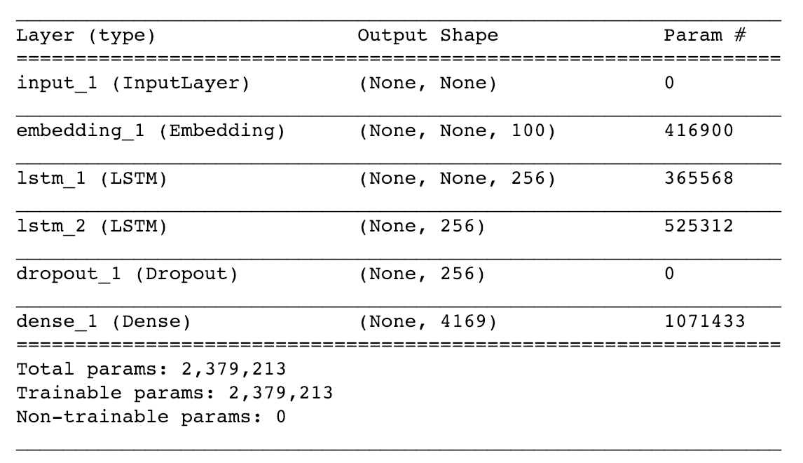
Figure 6-12. A stacked LSTM network

The code to build the stacked LSTM network is given in Example 6-5.

text_in = Input(shape = (None,))
    embedding = Embedding(total_words, embedding_size)
    x = embedding(text_in)
    x = LSTM(n_units, return_sequences = True)(x)
    x = LSTM(n_units)(x)
    x = Dropout(0.2)(x)
    text_out = Dense(total_words, activation = 'softmax')(x)

    model = Model(text_in, text_out)

Gated Recurrent Units

Another type of commonly used RNN layer is the gated recurrent unit (GRU).² The key differences from the LSTM unit are as follows:

1. The forget and input gates are replaced by reset and update gates.

2. There is no cell state or output gate, only a hidden state that is output from the cell.

The hidden state is updated in four steps, as illustrated in Figure 6-13.

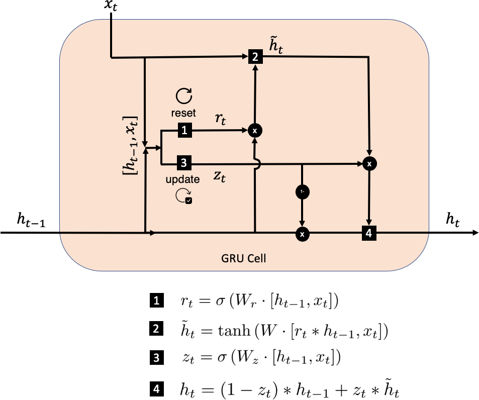
Figure 6-13. A single GRU cell

The process is as follows:

1. The hidden state of the previous timestep, h_t–1, and the current word embedding, x_t, are concatenated and used to create the reset gate. This gate is a dense layer, with weights matrix W_r and a sigmoid activation function. The resulting vector, r_t, has a length equal to the number of units in the cell and stores values between 0 and 1 that determine how much of the previous hidden state, h_t–1, should be carried forward into the calculation for the new beliefs of the cell.

2. The reset gate is applied to the hidden state, h_t–1, and concatenated with the current word embedding, x_t. This vector is then fed to a dense layer with weights matrix W and a tanh activation function to generate a vector, ${\tilde{h}}_t$, that stores the new beliefs of the cell. It has length equal to the number of units in the cell and stores values between –1 and 1.

3. The concatenation of the hidden state of the previous timestep, h_t–1, and the current word embedding, x_t, are also used to create the update gate. This gate is a dense layer with weights matrix W_z and a sigmoid activation. The resulting vector, z_t, has length equal to the number of units in the cell and stores values between 0 and 1, which are used to determine how much of the new beliefs, ${\tilde{h}}_t$, to blend into the current hidden state, h_t–1.

4. The new beliefs of the cell ${\tilde{h}}_t$ and the current hidden state, h_t–1, are blended in a proportion determined by the update gate, z_t, to produce the updated hidden state, h_t, that is output from the cell.

Bidirectional Cells

For prediction problems where the entire text is available to the model at inference time, there is no reason to process the sequence only in the forward direction—it could just as well be processed backwards. A bidirectional layer takes advantage of this by storing two sets of hidden states: one that is produced as a result of the sequence being processed in the usual forward direction and another that is produced when the sequence is processed backwards. This way, the layer can learn from information both preceding and succeeding the given timestep.

In Keras, this is implemented as a wrapper around a recurrent layer, as shown here:

layer = Bidirectional(GRU(100))

The hidden states in the resulting layer are vectors of length equal to double the number of units in the wrapped cell (a concatenation of the forward and backward hidden states). Thus, in this example the hidden states of the layer are vectors of length 200.

A Question-Answer Dataset

We’ll be using the Maluuba NewsQA dataset, which you can download by following the set of instructions on GitHub.

The resulting train.csv, test.csv, and dev.csv files should be placed in the ./data/qa/ folder inside the book repository. These files all have the same column structure, as follows:

story_id

A unique identifier for the story.

story_text

The text of the story (e.g., “The winning goal was scored by 23-year-old striker Joe Bloggs during the match…”).

question

A question that could be asked about the story text (e.g., “How much did the striker cost?”).

answer_token_ranges

The token positions of the answer in the story text (e.g., 24:27). There might be multiple ranges (comma separated) if the answer appears multiple times in the story.

This raw data is processed and tokenized so that is it able to be used as input to our model. After this transformation, each observation in the training set consists of the following five features:

document_tokens

The tokenized story text (e.g., [1, 4633, 7, 66, 11, ...]), clipped/padded with zeros to be of length max_document_length (a parameter).

question_input_tokens

The tokenized question (e.g., [2, 39, 1, 52, ...]), padded with zeros to be of length max_question_length (another parameter).

question_output_tokens

The tokenized question, offset by one timestep (e.g., [39, 1, 52, 1866, ...], padded with zeros to be of length max_question_length.

answer_masks

A binary mask matrix having shape [max_answer_length, max_document_length]. The [i, j] value of the matrix is 1 if the ith word of the answer to the question is located at the jth word of the document and 0 otherwise.

answer_labels

A binary vector of length max_document_length (e.g., [0, 1, 1, 0, ...]). The ith element of the vector is 1 if the ith word of the document could be considered part of an answer and 0 otherwise.

Let’s now take a look at the model architecture that is able to generate question-answer pairs from a given block of text.

Model Architecture

Figure 6-15 shows the overall model architecture that we will be building. Don’t worry if this looks intimidating! It’s only built from elements that we have seen already and we will be walking through the architecture step by step in this section.

Figure 6-15. The architecture for generating question–answer pairs; input data is shown in green bordered boxes

Let’s start by taking a look at the Keras code that builds the part of the model at the top of the diagram, which predicts if each word in the document is part of an answer or not. This code is shown in Example 6-6. You can also follow along with the accompanying notebook in the book repository, 06_02_qa_train.ipynb.

from keras.layers import Input, Embedding, GRU, Bidirectional, Dense, Lambda
from keras.models import Model, load_model
import keras.backend as K
from qgen.embedding import glove

#### PARAMETERS ####

VOCAB_SIZE = glove.shape[0] # 9984
EMBEDDING_DIMENS = glove.shape[1] # 100

GRU_UNITS = 100
DOC_SIZE = None
ANSWER_SIZE = None
Q_SIZE = None

document_tokens = Input(shape=(DOC_SIZE,), name="document_tokens") 

embedding = Embedding(input_dim = VOCAB_SIZE, output_dim = EMBEDDING_DIMENS
	, weights=[glove], mask_zero = True, name = 'embedding') 
document_emb = embedding(document_tokens)

answer_outputs = Bidirectional(GRU(GRU_UNITS, return_sequences=True)
	, name = 'answer_outputs')(document__emb) 
answer_tags = Dense(2, activation = 'softmax'
    , name = 'answer_tags')(answer_outputs) 

The document tokens are provided as input to the model. Here, we use the variable DOC_SIZE to describe the size of this input, but the variable is actually set to None. This is because the architecture of the model isn’t dependent on the length of the input sequence—the number of cells in the layer will adapt to equal the length of the input sequence, so we don’t need to specify it explicitly.

The embedding layer is initialized with GloVe word vectors (explained in the following sidebar).

The recurrent layer is a bidirectional GRU that returns the hidden state at each timestep.

The output Dense layer is connected to the hidden state at each timestep and has only two units, with a softmax activation, representing the probability that each word is part of an answer (1) or is not part of an answer (0).

To work with the GloVe word vectors within this project, download the file glove.6B.100d.txt (6 billion words each with an embedding of length 100) from the GloVe project website and then run the following Python script from the book repository to trim this file to only include words that are present in the training corpus:

python ./utils/write.py

The second part of the model is the encoder–decoder network that takes a given answer and tries to formulate a matching question (the bottom part of Figure 6-15).

The Keras code for this part of the network is given in Example 6-7.

encoder_input_mask = Input(shape=(ANSWER_SIZE, DOC_SIZE)
	, name="encoder_input_mask")
encoder_inputs = Lambda(lambda x: K.batch_dot(x[0], x[1])
	, name="encoder_inputs")([encoder_input_mask, answer_outputs])
encoder_cell = GRU(2 * GRU_UNITS, name = 'encoder_cell')(encoder_inputs) 

decoder_inputs = Input(shape=(Q_SIZE,), name="decoder_inputs") 
decoder_emb = embedding(decoder_inputs) 
decoder_emb.trainable = False
decoder_cell = GRU(2 * GRU_UNITS, return_sequences = True, name = 'decoder_cell')
decoder_states = decoder_cell(decoder_emb, initial_state = [encoder_cell]) 

decoder_projection = Dense(VOCAB_SIZE, name = 'decoder_projection'
	, activation = 'softmax', use_bias = False)
decoder_outputs = decoder_projection(decoder_states) 

total_model = Model([document_tokens, decoder_inputs, encoder_input_mask]
	, [answer_tags, decoder_outputs])
answer_model = Model(document_tokens, [answer_tags])
decoder_initial_state_model = Model([document_tokens, encoder_input_mask]
	, [encoder_cell])

The answer mask is passed as an input to the model—this allows us to pass the hidden states from a single answer range through to the encoder–decoder. This is achieved using a Lambda layer.

The encoder is a GRU layer that is fed the hidden states for the given answer range as input data.

The input data to the decoder is the question matching the given answer range.

The question word tokens are passed through the same embedding layer used in the answer identification model.

The decoder is a GRU layer and is initialized with the final hidden state from the encoder.

The hidden states of the decoder are passed through a Dense layer to generate a distribution over the entire vocabulary for the next word in the sequence.

This completes our network for question–answer pair generation. To train the network, we pass the document text, question text, and answer masks as input data in batches and minimize the cross-entropy loss on both the answer position prediction and question word generation, weighted equally.

Inference

To test the model on an input document sequence that it has never seen before, we need to run the following process:

1. Feed the document string to the answer generator to produce sample positions for answers in the document.

2. Choose one of these answer blocks to carry forward to the encoder–decoder question generator (i.e., create the appropriate answer mask).

3. Feed the document and answer mask to the encoder to generate the initial state for the decoder.

4. Initialize the decoder with this initial state and feed in the <START> token to generate the first word of the question. Continue this process, feeding in generated words one by one until the <END> token is predicted by the model.

As discussed previously, during training the model uses teacher forcing to feed the ground-truth words (rather than the predicted next words) back into the decoder cell. However during inference the model must generate a question by itself, so we want to be able to feed the predicted words back into the decoder cell while retaining its hidden state.

One way we can achieve this is by defining an additional Keras model (question_model) that accepts the current word token and current decoder hidden state as input, and outputs the predicted next word distribution and updated decoder hidden state. This is shown in Example 6-8.

decoder_inputs_dynamic = Input(shape=(1,), name="decoder_inputs_dynamic")
decoder_emb_dynamic = embedding(decoder_inputs_dynamic)
decoder_init_state_dynamic = Input(shape=(2 * GRU_UNITS,)
	, name = 'decoder_init_state_dynamic')
decoder_states_dynamic = decoder_cell(decoder_emb_dynamic
	, initial_state = [decoder_init_state_dynamic])
decoder_outputs_dynamic = decoder_projection(decoder_states_dynamic)

question_model = Model([decoder_inputs_dynamic, decoder_init_state_dynamic]
    , [decoder_outputs_dynamic, decoder_states_dynamic])

We can then use this model in a loop to generate the output question word by word, as shown in Example 6-9.

test_data_gen = test_data()
batch = next(test_data_gen)
answer_preds = answer_model.predict(batch["document_tokens"])

idx = 0
start_answer = 37
end_answer = 39

answers = [[0] * len(answer_preds[idx])]
for i in range(start_answer, end_answer + 1):
    answers[idx][i] = 1

answer_batch = expand_answers(batch, answers)

next_decoder_init_state = decoder_initial_state_model.predict(
	[answer_batch['document_tokens'][[idx]], answer_batch['answer_masks'][[idx]]])

word_tokens = [START_TOKEN]
questions = [look_up_token(START_TOKEN)]

ended = False

while not ended:

        word_preds, next_decoder_init_state = question_model.predict(
	[word_tokens, next_decoder_init_state])

        next_decoder_init_state = np.squeeze(next_decoder_init_state, axis = 1)
        word_tokens = np.argmax(word_preds, 2)[0]

        questions.append(look_up_token(word_tokens[0]))

        if word_tokens[0] == END_TOKEN:
                ended = True

questions = ' '.join(questions)

Model Results

Sample results from the model are shown in Figure 6-16 (see also the accompanying notebook in the book repository, 06_03_qa_analysis.ipynb). The chart on the right shows the probability of each word in the document forming part of an answer, according to the model. These answer phrases are then fed to the question generator and the output of this model is shown on the lefthand side of the diagram (“Predicted Question”).

First, notice how the answer generator is able to accurately identify which words in the document are most likely to be contained in an answer. This is already quite impressive given that it has never seen this text before and also may not have seen certain words from the document that are included in the answer, such as Bloggs. It is able to understand from the context that this is likely to be the surname of a person and therefore likely to form part of an answer.

Figure 6-16. Sample results from the model

The encoder extracts the context from each of these possible answers, so that the decoder is able to generate suitable questions. It is remarkable that the encoder is able to capture that the person mentioned in the first answer, 23-year-old striker Joe Bloggs, would probably have a matching question relating to his goal-scoring abilities, and is able to pass this context on to the decoder so that it can generate the question “who scored the <UNK> ?” rather than, for example, “who is the president ?”

The decoder has finished this question with the tag <UNK>, but not because it doesn’t know what to do next—it is predicting that the word that follows is likely to be from outside the core vocabulary. We shouldn’t be surprised that the model resorts to using the tag <UNK> in this context, as many of the niche words in the original corpus would be tokenized this way.

We can see that in each case, the decoder chooses the correct “type” of question—who, how much, or when—depending on the type of answer. There are still some problems though, such as asking how much money did he lose ? rather than how much money was paid for the striker ?. This is understandable, as the decoder only has the final encoder state to work with and cannot reference the original document for extra information.

There are several extensions to encoder–decoder networks that improve the accuracy and generative power of the model. Two of the most widely used are pointer networks⁴ and attention mechanisms.⁵ Pointer networks give the model the ability to “point” at specific words in the input text to include in the generated question, rather than only relying on the words in the known vocabulary. This helps to solve the <UNK> problem mentioned earlier. We shall explore attention mechanisms in detail in the next chapter.