
Chapter 8. Play
In March 2018, David Ha and Jürgen Schmidhuber published their “World Models” paper.1 The paper showed how it is possible to train a model that can learn how to perform a particular task through experimentation within its own generative hallucinated dreams, rather than inside the environment itself. It is an excellent example of how generative modeling can be used to solve practical problems, when applied alongside other machine learning techniques such as reinforcement learning.
A key component of the architecture is a generative model that can construct a probability distribution for the next possible state, given the current state and action. Having built up an understanding of the underlying physics of the environment through random movements, the model is then able to train itself from scratch on a new task, entirely within its own internal representation of the environment. This approach led to world-best scores for both of the tasks on which it was tested.
In this chapter, we will explore the model in detail and show how it is possible to create your own version of this amazing cutting-edge technology.
Based on the original paper, we will be building a reinforcement learning algorithm that learns how to drive a car around a racetrack as fast as possible. While we will be using a 2D computer simulation as our environment, the same technique could also be applied to real-world scenarios where testing strategies in the live environment is expensive or infeasible.
Before we start building the model, however, we need to take a closer look at the concept of reinforcement learning and the OpenAI Gym platform.
Reinforcement Learning
Reinforcement learning can be defined as follows:
Reinforcement learning (RL) is a field of machine learning that aims to train an agent to perform optimally within a given environment, with respect to a particular goal.
While both discriminative modeling and generative modeling aim to minimize a loss function over a dataset of observations, reinforcement learning aims to maximize the long-term reward of an agent in a given environment. It is often described as one of the three major branches of machine learning, alongside supervised learning (predicting using labeled data) and unsupervised learning (learning structure from unlabeled data).
Let’s first introduce some key terminology relating to reinforcement learning:
- Environment
-
The world in which the agent operates. It defines the set of rules that govern the game state update process and reward allocation, given the agent’s previous action and current game state. For example, if we were teaching a reinforcement learning algorithm to play chess, the environment would consist of the rules that govern how a given action (e.g., the move
e4) affects the next game state (the new positions of the pieces on the board) and would also specify how to assess if a given position is checkmate and allocate the winning player a reward of 1 after the winning move. - Agent
-
The entity that takes actions in the environment.
- Game state
-
The data that represents a particular situation that the agent may encounter (also just called a state), for example, a particular chessboard configuration with accompanying game information such as which player will make the next move.
- Action
-
A feasible move that an agent can make.
- Reward
-
The value given back to the agent by the environment after an action has been taken. The agent aims to maximize the long-term sum of its rewards. For example, in a game of chess, checkmating the opponent’s king has a reward of 1 and every other move has a reward of 0. Other games have rewards constantly awarded throughout the episode (e.g., points in a game of Space Invaders).
- Episode
-
One run of an agent in the environment; this is also called a rollout.
- Timestep
-
For a discrete event environment, all states, actions, and rewards are subscripted to show their value at timestep t.
The relationship between these definitions is shown in Figure 8-1.
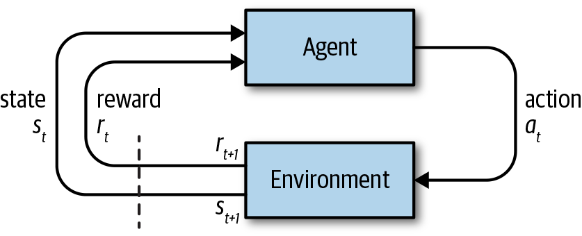
Figure 8-1. Reinforcement learning diagram
The environment is first initialized with a current game state, s0. At timestep t, the agent receives the current game state st and uses this to decide its next best action at, which it then performs. Given this action, the environment then calculates the next state st + 1 and reward rt + 1 and passes these back to the agent, for the cycle to begin again. The cycle continues until the end criterion of the episode is met (e.g., a given number of timesteps elapse or the agent wins/loses).
How can we design an agent to maximize the sum of rewards in a given environment? We could build an agent that contains a set of rules for how to respond to any given game state. However, this quickly becomes infeasible as the environment becomes more complex and doesn’t ever allow us to build an agent that has superhuman ability in a particular task, as we are hardcoding the rules. Reinforcement learning involves creating an agent that can learn optimal strategies by itself in complex environments through repeated play—this is what we will be using in this chapter to build our agent.
I’ll now introduce OpenAI Gym, home of the CarRacing environment that we will use to simulate a car driving around a track.
OpenAI Gym
OpenAI Gym is a toolkit for developing reinforcement learning algorithms that is available as a Python library.
Contained within the library are several classic reinforcement learning environments, such as CartPole and Pong, as well as environments that present more complex challenges, such as training an agent to walk on uneven terrain or win an Atari game. All of the environments provide a step method through which you can submit a given action; the environment will return the next state and the reward. By repeatedly calling the step method with the actions chosen by the agent, you can play out an episode in the environment.
In addition to the abstract mechanics of each environment, OpenAI Gym also provides graphics that allow you to watch your agent perform in a given environment. This is useful for debugging and finding areas where your agent could improve.
We will make use of the CarRacing environment within OpenAI Gym. Let’s see how the game state, action, reward, and episode are defined for this environment:
- Game state
-
A 64 × 64–pixel RGB image depicting an overhead view of the track and car.
- Action
-
A set of three values: the steering direction (–1 to 1), acceleration (0 to 1), and braking (0 to 1). The agent must set all three values at each timestep.
- Reward
-
A negative penalty of –0.1 for each timestep taken and a positive reward of 1000/N if a new track tile is visited, where N is the total number of tiles that make up the track.
- Episode
-
The episode ends when either the car completes the track, drives off the edge of the environment, or 3,000 timesteps have elapsed.
These concepts are shown on a graphical representation of a game state in Figure 8-2. Note that the car doesn’t see the track from its point of view, but instead we should imagine an agent floating above the track controlling the car from a bird’s-eye view.

Figure 8-2. A graphical representation of one game state in the CarRacing environment
World Model Architecture
We’ll now cover a high-level overview of the entire architecture that we will be using to build the agent that learns through reinforcement learning, before we explore the detailed steps required to build each component.
The solution consists of three distinct parts, as shown in Figure 8-3, that are trained separately:
- V
-
A variational autoencoder.
- M
-
A recurrent neural network with a mixture density network (MDN-RNN).
- C
-
A controller.

Figure 8-3. World model architecture diagram
The Variational Autoencoder
When you make decisions while driving, you don’t actively analyze every single pixel in your view—instead, you condense the visual information into a smaller number of latent entities, such as the straightness of the road, upcoming bends, and your position relative to the road, to inform your next action.
We saw in Chapter 3 how a VAE can take a high-dimensional input image and condense it into a latent random variable that approximately follows a standard multivariate normal distribution, through minimization of the reconstruction error and KL divergence. This ensures that the latent space is continuous and that we are able to easily sample from it to to generate meaningful new observations.
In the car racing example, the VAE condenses the 64 × 64 × 3 (RGB) input image into a 32-dimensional normally distributed random variable, parameterized by two variables, mu and log_var. Here, log_var is the logarithm of the variance of the distribution.
We can sample from this distribution to produce a latent vector z that represents the current state. This is passed on to the next part of the network, the MDN-RNN.
The MDN-RNN
As you drive, each subsequent observation isn’t a complete surprise to you. If the current observation suggests a left turn in the road ahead and you turn the wheel to the left, you expect the next observation to show that you are still in line with the road.
If you didn’t have this ability, your driving would probably snake all over the road as you wouldn’t be able see that a slight deviation from the center is going to be worse in the next timestep unless you do something about it now.
This forward thinking is the job of the MDN-RNN, a network that tries to predict the distribution of the next latent state based on the previous latent state and the previous action.
Specifically, the MDN-RNN is an LSTM layer with 256 hidden units followed by a mixture density network (MDN) output layer that allows for the fact that the next latent state could actually be drawn from any one of several normal distributions.
The same technique was applied by one of the authors of the “World Models” paper, David Ha, to a handwriting generation task, as shown in Figure 8-4, to describe the fact that the next pen point could land in any one of the distinct red areas.

Figure 8-4. MDN for handwriting generation
In the car racing example, we allow for each element of the next observed latent state to be drawn from any one of five normal distributions.
The Controller
Until this point, we haven’t mentioned anything about choosing an action. That responsibility lies with the controller.
The controller is a densely connected neural network, where the input is a concatenation of z (the current latent state sampled from the distribution encoded by the VAE) and the hidden state of the RNN. The three output neurons correspond to the three actions (turn, accelerate, brake) and are scaled to fall in the appropriate ranges.
We will need to train the controller using reinforcement learning as there is no training dataset that will tell us that a certain action is good and another is bad. Instead, the agent will need to discover this for itself through repeated experimentation.
As we shall see later in the chapter, the crux of the “World Models” paper is that it demonstrates how this reinforcement learning can take place within the agent’s own generative model of the environment, rather than the OpenAI Gym environment. In other words, it takes place in the agent’s hallucinated version of how the environment behaves, rather than the real thing.
To understand the different roles of the three components and how they work together, we can imagine a dialogue between them:
VAE (looking at latest 64 × 64 × 3 observation): This looks like a straight road, with a slight left bend approaching, with the car facing in the direction of the road (
z).RNN: Based on that description (
z) and the fact that the controller chose to accelerate hard at the last timestep (action), I will update my hidden state so that the next observation is predicted to still be a straight road, but with slightly more left turn in view.Controller: Based on the description from the VAE (
z) and the current hidden state from the RNN (h), my neural network outputs[0.34, 0.8, 0]as the next action.
The action from the controller is then passed to the environment, which returns an updated observation, and the cycle begins again.
For further information on the model, there is also an excellent interactive explanation available online.
Setup
We are now ready to start exploring how to build and train this model in Keras. If you’ve got a high-spec laptop, you can run the solution locally, but I’d recommend using cloud resources such as Google Cloud Compute Engine for access to powerful machines that you can use in short bursts.
Note
The following code has been tested on Ubuntu 16.04, so it is specific to a Linux terminal.
First install the following libraries:
sudo apt-get install cmake swig python3-dev
	zlib1g-dev python-opengl mpich xvfb
	xserver-xephyr vnc4server
Then clone the following repository:
git clone https://github.com/AppliedDataSciencePartners/WorldModels.git
As the codebase for this project is stored separately from the book repository, I suggest creating a separate virtual environment to work in:
mkvirtualenv worldmodels
cd WorldModels
pip install -r requirements.txt
Now you’re good to go!
Training Process Overview
Here’s an overview of the five-step training process:
-
Collect random rollout data Here, the agent does not care about the given task, but instead simply explores the environment at random. This will be conducted using OpenAI Gym to simulate multiple episodes and store the observed state, action, and reward at each timestep. The idea here is to build up a dataset of how the physics of the environment works, which the VAE can then learn from to capture the states efficiently as latent vectors. The MDN-RNN can then subsequently learn how the latent vectors evolve over time.
-
Train the VAE Using the randomly collected data, we train a VAE on the observation images.
-
Collect data to train the MDN-RNN Once we have a trained VAE, we use it to encode each of the collected observations into
muandlog_varvectors, which are saved alongside the current action and reward. -
Train the MDN-RNN We take batches of 100 episodes and load the corresponding
mu,log_var,action, andrewardvariables at each timestep that were generated in step 3. We then sample azvector from themuandlog_varvectors. Given the currentzvector,action, andreward, the MDN-RNN is then trained to predict the subsequentzvector andreward. -
Train the controller With a trained VAE and RNN, we can now train the controller to output an action given the current
zand hidden state,h, of the RNN. The controller uses an evolutionary algorithm, CMA-ES (Covariance Matrix Adaptation Evolution Strategy), as its optimizer. The algorithm rewards matrix weightings that generate actions that lead to overall high scores on the task, so that future generations are also likely to inherit this desired behavior.
Let’s now take a closer look at each of these steps in more detail.
Collecting Random Rollout Data
To start collecting data, run the following command from your terminal:
bash 01_generate_data.sh <env_name> <parallel_process> <episodes_per_process>
<render> <action_refresh_rate>
where the parameters are as follows:
<env_name>-
The name of the environment used by the
make_envfunction (e.g.,car_racing). <parallel_process>-
The number of processes to run (e.g.,
8for an 8-core machine). <episodes_per_process>-
How many episodes each process should run (e.g.,
125, so 8 processes would create 1,000 episodes overall). <max_timesteps>-
The maximum number of timesteps per episode (e.g., 300).
<render>-
1to render the rollout process in a window (otherwise0). <action_refresh_rate>-
The number of timesteps to freeze the current action for before changing. This prevents the action from changing too rapidly for the car to make progress.
For example, on an 8-core machine, you could run:
bash 01_generate_data.sh car_racing812530005
This would start 8 processes running in parallel, each simulating 125 episodes, with a maximum of 300 timesteps each and an action refresh rate of 5 timesteps.
Each process calls the Python file 01_generate_data.py. The key part of the script is outlined in Example 8-1.
Example 8-1. 01_generate_data.py excerpt
# ...DIR_NAME='./data/rollout/'env=make_env(current_env_name)s=0whiles<total_episodes:episode_id=random.randint(0,2**31-1)filename=DIR_NAME+str(episode_id)+".npz"observation=env.reset()env.render()t=0obs_sequence=[]action_sequence=[]reward_sequence=[]done_sequence=[]reward=-0.1done=Falsewhilet<time_steps:ift%action_refresh_rate==0:action=config.generate_data_action(t,env)observation=config.adjust_obs(observation)obs_sequence.append(observation)action_sequence.append(action)reward_sequence.append(reward)done_sequence.append(done)observation,reward,done,info=env.step(action)t=t+1("Episode {} finished after {} timesteps".format(s,t))np.savez_compressed(filename,obs=obs_sequence,action=action_sequence,reward=reward_sequence,done=done_sequence)s=s+1env.close()

make_envis a custom function in the repository that creates the appropriate OpenAI Gym environment. In this case, we are creating theCarRacingenvironment, with a few tweaks. The environment file is stored in the custom_envs folder.
generate_data_actionis a custom function that stores the rules for generating random actions.
The observations that are returned by the environment are scaled between 0 and 255. We want observations that are scaled between 0 and 1, so this function is simply a division by 255.

Every OpenAI Gym environment includes a
stepmethod. This returns the next observation, reward, and done flag, given an action.
We save each episode as an individual file inside the ./data/rollout/ directory.
Figure 8-5 shows an excerpt from frames 40 to 59 of one episode, as the car approaches a corner, alongside the randomly chosen action and reward. Note how the reward changes to 3.22 as the car rolls over new track tiles but is otherwise –0.1. Also, the action changes every five frames as the action_refresh_rate is 5.

Figure 8-5. Frames 40 to 59 of one episode
Training the VAE
We can now build a generative model (a VAE) on this collected data.
Remember, the aim of the VAE is to allow us to collapse one 64 × 64 × 3 image into a normally distributed random variable, whose distribution is parameterized by two vectors, mu and log_var. Each of these vectors is of length 32.
To start training the VAE, run the following command from your terminal:
python 02_train_vae.py --new_model[--N][--epochs]
where the parameters are as follows:
--new_model-
Whether the model should be trained from scratch. Set this flag initially; if it’s not set, the code will look for a ./vae/vae.json file and continue training a previous model.
--N(optional)-
The number of episodes to use when training the VAE (e.g.,
1000—the VAE does not need to use all the episodes to achieve good results, so to speed up training you can use only a sample of the episodes). --epochs(optional)-
The number of training epochs (e.g.,
3).
The output of the training process should be as shown in Figure 8-6. A file storing the weights of the trained network is saved to ./vae/vae.json every epoch.
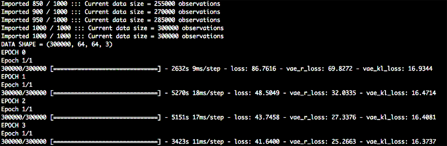
Figure 8-6. Training the VAE
The VAE Architecture
As we have seen previously, the Keras functional API allows us to not only define the full VAE model that will be trained, but also additional models that reference the encoder and decoder parts of the trained network separately. These will be useful when we want to encode a specific image, or decode a given z vector, for example.
In this example, we define four different models on the VAE:
full_model-
This is the full end-to-end model that is trained.
encoder-
This accepts a 64 × 64 × 3 observation as input and outputs a sampled
zvector. If you run thepredictmethod of this model for the same input multiple times, you will get different output, since even though themuandlog_varvalues are constant, the randomly sampledzvector will be different each time. encoder_mu_log_var-
This accepts a 64 × 64 × 3 observation as input and outputs the
muandlog_varvectors corresponding to this input. Unlike with thevae_encodermodel, if you run thepredictmethod of this model multiple times, you will always get the same output: amuvector of length 32 and alog_varvector of length 32. decoder-
This accepts a
zvector as input and returns the reconstructed 64 × 64 × 3 observation.
A diagram of the VAE is given in Figure 8-7. You can play around with the VAE architecture by editing the ./vae/arch.py file. This is where the VAE class and parameters of the neural network are defined.

Figure 8-7. The VAE architecture for the “World Models” paper
Exploring the VAE
We’ll now take a look at the output from the predict methods of the different models built on the VAE to see how they differ, and then see how the VAE can be used to generate completely new track observations.
The full model
If we feed the full_model with an observation, it is able to reconstruct an accurate representation of the image, as shown in Figure 8-8. This is useful to visually check that the VAE is working correctly.

Figure 8-8. The input and output from the full VAE model
The encoder models
If we feed the encoder_mu_log_var model with an observation, the output is the generated mu and log_var vectors describing a multivariate normal distribution.
The encoder model goes one step further by sampling a particular z vector from this distribution.
The output from the two encoder models is shown in Figure 8-9.

Figure 8-9. The output from the encoder models
It is interesting to plot the value of mu and log_var for each of the 32 dimensions (Figure 8-10), for a particular observation. Notice how only 12 of the 32 dimensions differ significantly from the standard normal distribution (mu = 0, log_var = 0). This is because the VAE is trying to minimize the KL divergence, so it tries to differ from the standard normal distribution in as few dimensions as possible. It has decided that 12 dimensions are enough to capture sufficient information about the observations for accurate reconstruction.

Figure 8-10. A plot of mu (blue line) and log_var (orange line) for each of the 32 dimensions of a particular observation
The decoder model
The decoder model accepts a z vector as input and reconstructs the original image. In Figure 8-11 we linearly interpolate two of the dimensions of z to show how each dimension appears to encode a particular aspect of the track—for example, z[4] controls the immediate left/right direction of the track nearest the car and z[7] controls the sharpness of the approaching left turn.

Figure 8-11. A linear interpolation of two dimensions of z
This shows that the latent space that the VAE has learned is continuous and can be used to generate new track segments that have never before been observed by the agent.
Collecting Data to Train the RNN
Now that we have a trained VAE, we can use this to generate training data for our RNN.
In this step, we pass all of the random rollout data through the encoder_mu_log_var model and store the mu and log_var vectors corresponding to each observation. This encoded data, along with the already collected actions and rewards, will be used to train the MDN-RNN.
To start collecting data, run the following command from your terminal:
python 03_generate_rnn_data.py
Example 8-2 contains an excerpt from the 03_generate_data.py file that shows how the MDN-RNN training data is generated.
Example 8-2. Excerpt from 03_generate_data.py
defencode_episode(vae,episode):obs=episode['obs']action=episode['action']reward=episode['reward']done=episode['done']mu,log_var=vae.encoder_mu_log_var.predict(obs)done=done.astype(int)reward=np.where(reward>0,1,0)*np.where(done==0,1,0)initial_mu=mu[0,:]initial_log_var=log_var[0,:]return(mu,log_var,action,reward,done,initial_mu,initial_log_var)vae=VAE()vae.set_weights('./vae/weights.h5')forfileinfilelist:rollout_data=np.load(ROLLOUT_DIR_NAME+file)mu,log_var,action,reward,done,initial_mu,initial_log_var=encode_episode(vae,rollout_data)np.savez_compressed(SERIES_DIR_NAME+file,mu=mu,log_var=log_var,action=action,reward=reward,done=done)initial_mus.append(initial_mu)initial_log_vars.append(initial_log_var)np.savez_compressed(ROOT_DIR_NAME+'initial_z.npz',initial_mu=initial_mus,initial_log_var=initial_log_vars)
Here, we’re using the
encoder_mu_log_varmodel of the VAE to get themuandlog_varvectors for a particular observation.The reward value is transformed to be either 0 or 1, so that it can be used as input into the MDN-RNN.
We also save the initial
muandlog_varvectors into a separate file—this will be useful later, for initializing the dream environment.
Training the MDN-RNN
We can now train the MDN-RNN to predict the distribution of the next z vector and reward, given the current z value, current action, and previous reward.
The aim of the MDN-RNN is to predict one timestep ahead into the future—we can then use the internal hidden state of the LSTM as part of the input into the controller.
To start training the MDN-RNN, run the following command from your terminal:
python 04_train_rnn.py(--new_model)(--batch_size)(--steps)
where the parameters are as follows:
new_model-
Whether the model should be trained from scratch. Set this flag initially; if it’s not set, the code will look for a ./rnn/rnn.json file and continue training a previous model.
batch_size-
The number of episodes fed to the MDN-RNN in each training iteration.
steps-
The total number of training iterations.
The output of the training process is shown in Figure 8-12. A file storing the weights of the trained network is saved to ./rnn/rnn.json every 10 steps.

Figure 8-12. Training the MDN-RNN
The MDN-RNN Architecture
The architecture of the MDN-RNN is shown in Figure 8-13.

Figure 8-13. The MDN-RNN architecture
It consists of an LSTM layer (the RNN), followed by a densely connected layer (the MDN) that transforms the hidden state of the LSTM into the parameters of mixture distribution. Let’s walk through the network step by step.
The input to the LSTM layer is a vector of length 36—a concatenation of the encoded z vector (length 32) from the VAE, the current action (length 3), and the previous reward (length 1).
The output from the LSTM layer is a vector of length 256—one value for each LSTM cell in the layer. This is passed to the MDN, which is just a densely connected layer that transforms the vector of length 256 into a vector of length 481.
Why 481? Figure 8-14 explains the composition of the output from the MDN-RNN. Remember, the aim of a mixture density network is to model the fact that our next z could be drawn from one of several possible distributions with a certain probability. In the car racing example, we choose five normal distributions. How many parameters do we need to define these distributions? For each of the five mixtures, we need a mu and a log_sigma (to define the distribution) and a probability of this mixture being chosen (log_pi), for each of the 32 dimensions of z. This makes 5 × 3 × 32 = 480 parameters. The one extra parameter is for the reward prediction—more specifically, the log odds of reward at the next timestep.

Figure 8-14. The output from the mixture density network
Sampling the Next z and Reward from the MDN-RNN
We can sample from the MDN output to generate a prediction for the next z and reward at the following timestep, through the following process:
-
Split the 481-dimensional output vector into the 3 variables (
log_pi,mu,log_sigma) and the reward value. -
Exponentiate and scale
log_piso that it can be interpreted as 32 probability distributions over the 5 mixture indices. -
For each of the 32 dimensions of
z, sample from the distributions created fromlog_pi(i.e., choose which of the 5 distributions should be used for each dimension ofz). -
Fetch the corresponding values of
muandlog_sigmafor this distribution. -
Sample a value for each dimension of
zfrom the normal distribution parameterized by the chosen parameters ofmuandlog_sigmafor this dimension. -
If the reward log odds value is greater than 0, predict
1for the reward; otherwise, predict0.
The MDN-RNN Loss Function
The loss function for the MDN-RNN is the sum of the z vector reconstruction loss and the reward loss.
The excerpt from the rnn/arch.py file for the MDN-RNN in Example 8-3 shows how we construct the custom loss function in Keras.
Example 8-3. Excerpt from rnn/arch.py
defget_responses(self,y_true):z_true=y_true[:,:,:Z_DIM]rew_true=y_true[:,:,-1]returnz_true,rew_truedefget_mixture_coef(self,z_pred):log_pi,mu,log_sigma=tf.split(z_pred,3,1)log_pi=log_pi-K.log(K.sum(K.exp(log_pi),axis=1,keepdims=True))returnlog_pi,mu,log_sigmadeftf_lognormal(self,z_true,mu,log_sigma):logSqrtTwoPI=np.log(np.sqrt(2.0*np.pi))return-0.5*((z_true-mu)/K.exp(log_sigma))**2-log_sigma-logSqrtTwoPIdefrnn_z_loss(y_true,y_pred):z_true,rew_true=self.get_responses(y_true)d=normaldistribution_MIXTURES*Z_DIMz_pred=y_pred[:,:,:(3*d)]z_pred=K.reshape(z_pred,[-1,normaldistribution_MIXTURES*3])log_pi,mu,log_sigma=self.get_mixture_coef(z_pred)flat_z_true=K.reshape(z_true,[-1,1])z_loss=log_pi+self.tf_lognormal(flat_z_true,mu,log_sigma)z_loss=-K.log(K.sum(K.exp(z_loss),1,keepdims=True))z_loss=K.mean(z_loss)returnz_lossdefrnn_rew_loss(y_true,y_pred):z_true,rew_true=self.get_responses(y_true)#, done_trued=normaldistribution_MIXTURES*Z_DIMreward_pred=y_pred[:,:,-1]rew_loss=K.binary_crossentropy(rew_true,reward_pred,from_logits=True)rew_loss=K.mean(rew_loss)returnrew_lossdefrnn_loss(y_true,y_pred):z_loss=rnn_z_loss(y_true,y_pred)rew_loss=rnn_rew_loss(y_true,y_pred)returnZ_FACTOR*z_loss+REWARD_FACTOR*rew_lossopti=Adam(lr=LEARNING_RATE)model.compile(loss=rnn_loss,optimizer=opti,metrics=[rnn_z_loss,rnn_rew_loss])
Split the 481-dimensional output vector into the 3 variables (
log_pi,mu,log_sigma) and the reward value.This is the calculation of the
zvector reconstruction loss: the negative log-likelihood of observing the truez, under the mixture distribution parameterized by the output from the MDN-RNN. We want this value to be as large as possible, or equivalently, we seek to minimize the negative log likelihood.For the reward loss, we simply use the binary cross entropy between the true reward and the predicted log odds from the network.
The loss is the sum of the
zreconstruction loss and the reward loss—we set the weighting parametersZ_FACTORandREWARD_FACTORboth to1, though these can be adjusted to prioritize reconstruction loss or reward loss.
Notice that to train the MDN-RNN, we do not need to sample specific z vectors from the MDN output, but instead calculate the loss directly using the 481-dimensional output vector.
Training the Controller
The final step is to train the controller (the network that outputs the chosen action) using an evolutionary algorithm called CMA-ES (Covariance Matrix Adaptation Evolution Strategy).
To start training the controller, run the following command from your terminal (all on one line):
xvfb-run -a -s "-screen 0 1400x900x24" python 05_train_controller.py car_racing
  -n 16 -t 2 -e 4 --max_length 1000
where the parameters are as follows:
n-
The number of workers that will test solutions in parallel (this should be no greater than the number of cores on your machine)
t-
The number of solutions that each worker will be given to test at each generation
e-
The number of episodes that each solution will be tested against to calculate the average reward
max_length-
The maximum number of timeframes in each episode
eval_steps-
The number of generations between evaluations of the current best parameter set
The above command uses a virtual frame buffer (xvfb) to render the frames, so that the code can run on a Linux machine without a physical screen. The population size, pop_size = n * t.
The Controller Architecture
The architecture of the controller is very simple. It is a densely connected neural network with no hidden layer; it connects the input vector directly to the action vector.
The input vector is a concatenation of the current z vector (length 32) and the current hidden state of the LSTM (length 256), giving a vector of length 288. Since we are connecting each input unit directly to the 3 output action units, the total number of weights to tune is 288 × 3 = 864, plus 3 bias weights, giving 867 in total.
How should we train this network? Notice that this is not a supervised learning problem—we are not trying to predict the correct action. There is no training set of correct actions, as we do not know what the optimal action is for a given state of the environment. This is what distinguishes this as a reinforcement learning problem. We need the agent to discover the optimal values for the weights itself by experimenting within the environment and updating its weights based on received feedback.
Evolutionary strategies are becoming a popular choice for solving reinforcement learning problems, due to their simplicity, efficiency, and scalability. We shall use one particular strategy, known as CMA-ES.
CMA-ES
Evolutionary strategies generally adhere to the following process:
-
Create a population of agents and randomly initialize the parameters to be optimized for each agent.
-
Loop over the following:
-
Evaluate each agent in the environment, returning the average reward over multiple episodes.
-
Breed the agents with the best scores to create new members of the population.
-
Add randomness to the parameters of the new members.
-
Update the population pool by adding the newly created agents and removing poorly performing agents.
-
This is similar to the process through which animals evolve in nature—hence the name evolutionary strategies. “Breeding” in this context simply means combining the existing best-scoring agents such that the next generation are more likely to produce high-quality results, similar to their parents. As with all reinforcement learning solutions, there is a balance to be found between greedily searching for locally optimal solutions and exploring unknown areas of the parameter space for potentially better solutions. This is why it is important to add randomness to the population, to ensure we are not too narrow in our search field.
CMA-ES is just one form of evolutionary strategy. In short, it works by maintaining a normal distribution from which it can sample the parameters of new agents. At each generation, it updates the mean of the distribution to maximize the likelihood of sampling the high-scoring agents from the previous timestep. At the same time, it updates the covariance matrix of the distribution to maximize the likelihood of sampling the high-scoring agents, given the previous mean. It can be thought of as a form of naturally arising gradient descent, but with the added benefit that it is derivative-free, meaning that we do not need to calculate or estimate costly gradients.
One generation of the algorithm demonstrated on a toy example is shown in Figure 8-15. Here we are trying to find the minimum point of a highly nonlinear function in two dimensions—the value of the function in the red/black areas of the image is greater than the value of the function in the white/yellow parts of the image.

Figure 8-15. One update step from the CMA-ES algorithm2
The steps are as follows:
-
We start with a randomly generated 2D normal distribution and sample a population of candidates, shown in blue.
-
We then calculate the value of the function for each candidate and isolate the best 25%, shown in purple—we’ll call this set of points
P. -
We set the mean of the new normal distribution to be the mean of the points in
P. This can be thought of as the breeding stage, wherein we only use the best candidates to generate a new mean for the distribution. We also set the covariance matrix of the new normal distribution to be the covariance matrix of the points inP, but use the existing mean in the covariance calculation rather than the current mean of the points inP. The larger the difference between the existing mean and the mean of the points inP, the wider the variance of the next normal distribution. This has the effect of naturally creating momentum in the search for the optimal parameters. -
We can then sample a new population of candidates from our new normal distribution with an updated mean and covariance matrix.
Figure 8-16 shows several generations of the process. See how the covariance widens as the mean moves in large steps toward the minimum, but narrows as the mean settles into the true minimum.

Figure 8-16. CMA-ES3
For the car racing task, we do not have a well-defined function to maximize, but instead an environment where the 867 parameters to be optimized determine how well the agent scores. Initially, some sets of parameters will, by random chance, generate scores that are higher than others and the algorithm will gradually move the normal distribution in the direction of those parameters that score highest in the environment.
Parallelizing CMA-ES
One of the great benefits of CMA-ES is that it can be easily parallelized using a Python library created by David Ha called es.py. The most time-consuming part of the algorithm is calculating the score for a given set of parameters, since it needs to simulate an agent with these parameters in the environment. However, this process can be parallelized, since there are no dependencies between individual simulations. In the codebase, we use a master/slave setup, where there is a master process that sends out parameter sets to be tested to many slave processes in parallel. The slave nodes return the results to the master, which accumulates the results and then passes the overall result of the generation to the CMA-ES object. This object updates the mean and covariance matrix of the normal distribution as per Figure 8-15 and provides the master with a new population to test. The loop then starts again. Figure 8-17 explains this in a diagram.

Figure 8-17. Parallelizing CMA-ES—here there is a population size of 8 and 4 slave nodes (so t = 2, the number of trials that each slave is responsible for)
The master asks the CMA-ES object (
es) for a set of parameters to trial.The master divides the parameters into the number of slave nodes available. Here, each of the four slave processes gets two parameter sets to trial.
The slave nodes run a worker process that loops over each set of parameters and runs several episodes for each. Here we run three episodes for each set of parameters.
The rewards from each episode are averaged to give a single score for each set of parameters.
The slave node returns the list of scores to the master.

The master groups all the scores together and sends this list to the
esobject.
The
esobject uses this list of rewards to calculate the new normal distribution as per Figure 8-15.
Output from the Controller Training
The output of the training process is shown in Figure 8-18. A file storing the weights of the trained network is saved every eval_steps generations.

Figure 8-18. Training the controller
Each line of the output represents one generation of training. The reported statistics for each generation are as follows:
-
Environment name (e.g.,
car_racing) -
Generation number (e.g.,
16) -
Current elapsed time in seconds (e.g.,
2395) -
Average reward of the generation (e.g.,
136.44) -
Minimum reward of the generation (e.g.,
33.28) -
Maximum reward of the generation (e.g.,
246.12) -
Standard deviation of the rewards (e.g.,
62.78) -
Current standard deviation factor of the ES process (initialized at
0.5and decays each timestep; e.g.,0.4604) -
Minimum timesteps taken before termination (e.g.,
1000.0) -
Maximum timesteps taken before termination (e.g.,
1000)
After eval_steps timesteps, each slave node evaluates the current best-scoring parameter set and returns the average rewards across several episodes. These rewards are again averaged to return the overall score for the parameter set.
After around 200 timesteps, the training process achieves an average reward score of 840 for the car racing task.
In-Dream Training
So far, the controller training has been conducted using the OpenAI Gym CarRacing environment to implement the step method that moves the simulation from one state to the next. This function calculates the next state and reward, given the current state of the environment and chosen action.
Notice how the step method performs a very similar function to the MDN-RNN in our model. Sampling from the MDN-RNN outputs a prediction for the next z and reward, given the current z and chosen action.
In fact, the MDN-RNN can be thought of as an environment in its own right, but operating in z-space rather than in the original image space. Incredibly, this means that we can actually substitute the real environment with a copy of the MDN-RNN and train the controller entirely within an MDN-RNN-inspired dream of how the environment should behave.
In other words, the MDN-RNN has learned enough about the general physics of the real environment from the original random movement dataset that it can be used as a proxy for the real environment when training the controller. This is quite remarkable—it means that the agent can train itself to learn a new task by thinking about how it can maximize reward in its dream environment, without ever having to test out strategies in the real world. It can then perform well at the task first time, having never attempted the task in reality.
This is one reason why the “World Models” paper is highly important and why generative modeling will almost certainly form a key component of artificial intelligence in the future.
A comparison of the architectures for training in the real environment and the dream environment follows: the real-world architecture is shown in Figure 8-19 and the in-dream training setup is illustrated in Figure 8-20.

Figure 8-19. Training the controller in the OpenAI Gym environment
Notice how in the dream architecture, the training of the controller is performed entirely in z-space without the need to ever decode the z vectors back into recognizable track images. We can of course do so, in order to visually inspect the performance of the agent, but it is not required for training.

Figure 8-20. Training the controller in the MDN-RNN dream environment
In-Dream Training the Controller
To train the controller using the dream environment, run the following command from your terminal (on one line):
xvfb-run -a -s "-screen 0 1400x900x24" python 05_train_controller.py car_racing
  -n 16 -t 2 -e 4 --max_length 1000 --dream_mode 1
This is the same command used to train the controller in the real environment, but with the added flag --dream_mode 1.
The output of the training process is shown in Figure 8-21.

Figure 8-21. Output from in-dream training
When training in the dream environment, the scores of each generation are given in terms of the average sum of the dream rewards (i.e., 0 or 1 at each timestep). However, the evaluation performed after every 10 generations is still conducted in the real environment and is therefore scored based on the sum of rewards from the OpenAI Gym environment, so that we can compare training methods.
After just 10 generations of training in the dream environment, the agent scores an average of 586.6 in the real environment. The car is able to drive accurately around the track and can handle most corners, except those that are especially sharp.
This is an amazing achievement—remember, when the controller was evaluated after 10 generations it had never attempted the task of driving fast around the track in the real environment. It had only ever driven around the environment randomly (to train the VAE and MDN-RNN) and then in its own dream environment to train the controller.
As a comparison, after 10 generations the agent trained in the real environment is barely able to move off the start line. Moreover, each generation of training in the dream environment is around 3–4 times faster than training in the real environment, since z and reward prediction by the MDN-RNN is faster than z and reward calculation by the OpenAI Gym environment.
Challenges of In-Dream Training
One of the challenges of training agents entirely within the MDN-RNN dream environment is overfitting. This occurs when the agent finds a strategy that is rewarding in the dream environment, but does not generalize well to the real environment, due to the MDN-RNN not fully capturing how the true environment behaves under certain conditions.
We can see this happening in Figure 8-21: after 20 generations, even though the in-dream scores continue to rise, the agent only scores 363.7 in the real environment, which is worse than its score after 10 generations.
The authors of the original “World Models” paper highlight this challenge and show how including a temperature parameter to control model uncertainty can help alleviate the problem. Increasing this parameter magnifies the variance when sampling z through the MDN-RNN, leading to more volatile rollouts when training in the dream environment. The controller receives higher rewards for safer strategies that encounter well-understood states and therefore tend to generalize better to the real environment. Increased temperature, however, needs to be balanced against not making the environment so volatile that the controller cannot learn any strategy, as there is not enough consistency in how the dream environment evolves over time.
In the original paper, the authors show this technique successfully applied to a different environment: DoomTakeCover, based around the computer game Doom. Figure 8-22 shows how changing the temperature parameter affects both the virtual (dream) score and the actual score in the real environment.

Figure 8-22. Using temperature to control dream environment volatility4
Summary
In this chapter we have seen how a generative model (a VAE) can be utilized within a reinforcement learning setting to enable an agent to learn an effective strategy by testing policies within its own generated dreams, rather than within the real environment.
The VAE is trained to learn a latent representation of the environment, which is then used as input to a recurrent neural network that forecasts future trajectories within the latent space.
Amazingly, the agent can then use this generative model as a pseudoenvironment to iteratively test policies, using an evolutionary methodology, which generalize well to the real environment.
1 David Ha and Jürgen Schmidhuber, “World Models,” 27 March 2018, https://arxiv.org/abs/1803.10122.
2 Reproduced with permission from David Ha, 2017, http://bit.ly/2XufRwq.
3 Source: https://en.wikipedia.org/wiki/CMA-ES.
4 Source: Ha and Schmidhuber, 2018.