SoX and LibROSA

Most of the audio processing that torchaudio carries out relies on two other pieces of software: SoX and LibROSA. LibROSA is a Python library for audio analysis, including generating mel spectrograms (You’ll see what these are a little later in the chapter), detecting beats, and even generating music.

SoX, on the other hand, is a program that you might already be familiar with if you’ve been using Linux for years. In fact, SoX is so old that it predates Linux itself; its first release was in July 1991, compared to the Linux debut in September 1991. I remember using it back in 1997 to convert WAV files into MP3s on my first ever Linux box. But it’s still useful!¹

If you’re installing torchaudio via conda, you can skip to the next section. If you’re using pip, you’ll probably need to install SoX itself. For a Red Hat-based system, enter the following:

yum install sox

Or on a Debian-based system, you’ll use this:

apt intall sox

Once SoX is installed, you can move on to obtaining torchaudio itself.

torchaudio

Installing torchaudio can be performed with either conda or pip:

conda install -c derickl torchaudio
pip install torchaudio

In comparison with torchvision, torchaudio is similar to torchtext in that it’s not quite as well loved, maintained, or documented. I’d expect this to change in the near future as PyTorch gets more popular and better text and audio handling pipelines are created. Still, torchaudio is plenty for our needs; we just have to write some custom dataloaders (which we didn’t have to do for audio or text processing).

Anyhow, the core of torchaudio is found within load() and save(). We’re concerned only with load() in this chapter, but you’ll need to use save() if you’re generating new audio from your input (e.g., a text-to-speech model). load() takes a file specified in filepath and returns a tensor representation of the audio file and the sample rate of that audio file as a separate variable.

We now have the means for loading one of the WAV files from the ESC-50 dataset and turning it into a tensor. Unlike our earlier work with text and images, we need to write a bit more code before we can get on with creating and training a model. We need to write a custom dataset.

Building an ESC-50 Dataset

We’ve talked about datasets in Chapter 2, but torchvision and torchtext did all the heavy lifting for us, so we didn’t have to worry too much about the details. As you may remember, a custom dataset has to implement two class methods, __getitem__ and __len__, so that the data loader can get a batch of tensors and their labels, as well as a total count of tensors in the dataset. We also have an __init__ method for setting up things like file paths that’ll be used over and over again.

Here’s our first pass at the ESC-50 dataset:

class ESC50(Dataset):

    def __init__(self,path):
        # Get directory listing from path
        files = Path(path).glob('*.wav')
        # Iterate through the listing and create a list of tuples (filename, label)
        self.items = [(f,int(f.name.split("-")[-1]
                    .replace(".wav",""))) for f in files]
        self.length = len(self.items)

    def __getitem__(self, index):
        filename, label = self.items[index]
        audio_tensor, sample_rate = torchaudio.load(filename)
        return audio_tensor, label

    def __len__(self):
        return self.length

The majority of the work in the class happens when a new instance of it is created. The __init__ method takes the path parameter, finds all the WAV files inside that path, and then produces tuples of (filename, label) by using the same string split we used earlier in the chapter to get the label of that audio sample. When PyTorch requests an item from the dataset, we index into the items list, use torchaudio.load to make torchaudio load in the audio file, turn it into a tensor, and then return both the tensor and the label.

And that’s enough for us to start with. For a sanity check, let’s create an ESC50 object and extract the first item:

test_esc50 = ESC50(PATH_TO_ESC50)
tensor, label = list(test_esc50)[0]

tensor
tensor([-0.0128, -0.0131, -0.0143,  ...,  0.0000,  0.0000,  0.0000])

tensor.shape
torch.Size([220500])

label
'15'

We can construct a data loader by using standard PyTorch constructs:

example_loader = torch.utils.data.DataLoader(test_esc50, batch_size = 64,
shuffle = True)

But before we do that, we have to go back to our data. As you might remember, we should always create training, validation, and test sets. At the moment, we have just one directory with all the data, which is no good for our purposes. A 60/20/20 split of data into training, validation, and test collections should suffice. Now, we could do this by taking random samples of our entire dataset (taking care to sample without replacement and making sure that our newly constructed datasets are still balanced), but again the ESC-50 dataset saves us from having to do much work. The compilers of the dataset separated the data into five equal balanced folds, indicated by the first digit in the filename. We’ll have folds 1,2,3 be the training set, 4 the validation set, and 5 the test set. But feel free to mix it up if you don’t want to be boring and consecutive! Move each of the folds to test, train, and validation directories:

mv 1* ../train
mv 2* ../train
mv 3* ../train
mv 4* ../valid
mv 5* ../test

Now we can create the individual datasets and loaders:

from pathlib import Path

bs=64
PATH_TO_ESC50 = Path.cwd() / 'esc50'
path =  'test.md'
test

train_esc50 = ESC50(PATH_TO_ESC50 / "train")
valid_esc50 = ESC50(PATH_TO_ESC50 / "valid")
test_esc50  = ESC50(PATH_TO_ESC50 / "test")

train_loader = torch.utils.data.DataLoader(train_esc50, batch_size = bs,
                shuffle = True)
valid_loader = torch.utils.data.DataLoader(valid_esc50, batch_size = bs,
                shuffle = True)
test_loader  = torch.utils.data.DataLoader(test_esc50, batch_size = bs,
                shuffle = True)

We have our data all set up, so we’re all ready to look at a classification model.

Mel Spectrograms

Traditionally, getting into the frequency domain requires applying the Fourier transform on the audio signal. We’re going to go beyond that a little by generating our spectrograms in the mel scale. The mel scale defines a scale of pitches that are equal in distance from another, where 1000 mels = 1000 Hz. This scale is commonly used in audio processing, especially in speech recognition and classification applications. Producing a mel spectrogram with LibROSA requires two lines of code:

sample_data, sr = librosa.load("ESC-50/train/1-100032-A-0.wav", sr=None)
spectrogram = librosa.feature.melspectrogram(sample_data, sr=sr)

This results in a NumPy array containing the spectrogram data. If we display this spectrogram as shown in Figure 6-4, we can see the frequencies in our sound:

librosa.display.specshow(spectrogram, sr=sr, x_axis='time', y_axis='mel')

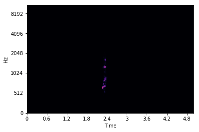
Figure 6-4. Mel spectrogram

However, not a lot of information is present in the image. We can do better! If we convert the spectrogram to a logarithmic scale, we can see a lot more of the audio’s structure, due to the scale being able to represent a wider range of values. And this is common enough in audio procressing that LibROSA includes a method for it:

log_spectrogram = librosa.power_to_db(spectrogram, ref=np.max)

This computes a scaling factor of 10 * log10(spectrogram / ref). ref defaults to 1.0, but here we’re passing in np.max() so that spectrogram / ref will fall within the range of [0,1]. Figure 6-5 shows the new spectrogram.

Figure 6-5. Log mel spectrogram

We now have a log-scaled mel spectrogram! If you call log_spectrogram.shape, you’ll see it’s a 2D tensor, which makes sense because we’ve plotted images with the tensor. We could create a new neural network architecture and feed this new data into it, but I have a diabolical trick up my sleeve. We literally just generated images of the spectrogram data. Why don’t we work on those instead?

This might seem silly at first; after all, we have the underlying spectrogram data, and that’s more exact than the image representation (to our eyes, knowing that a data point is 58 rather than 60 means more to us than a different shade of, say, purple). And if we were starting from scratch, that’d definitely be the case. But! We have, just lying around the place, already-trained networks such as ResNet and Inception that we know are amazing at recognizing structure and other parts of images. We can construct image representations of our audio and use a pretrained network to make big jumps in accuracy with very little training by using the super power of transfer learning once again. This could be useful with our dataset, as we don’t have a lot of examples (only 2,000!) to train our network.

This trick can be employed across many disparate datasets. If you can find a way of cheaply turning your data into an image representation, it’s worth doing that and throwing a ResNet network against it to get a baseline of what transfer learning can do for you, so you know what you have to beat by using a different approach. Armed with this, let’s create a new dataset that will generate these images for us on demand.

A New Dataset

Now throw away the original ESC50 dataset class and build a new one, ESC50Spectrogram. Although this will share some code with the older class, quite a lot more is going on in the __get_item__ method in this version. We generate the spectrogram by using LibROSA, and then we do some fancy matplotlib footwork to get the data into a NumPy array. We apply the array to our transformation pipeline (which just uses ToTensor) and return that and the item’s label. Here’s the code:

class ESC50Spectrogram(Dataset):

def __init__(self,path):
    files = Path(path).glob('*.wav')
    self.items = [(f,int(f.name.split("-")[-1].replace(".wav","")))
                   for f in files]
    self.length = len(self.items)
    self.transforms = torchvision.transforms.Compose(
                 [torchvision.transforms.ToTensor()])

def __getitem__(self, index):
    filename, label = self.items[index]
    audio_tensor, sample_rate = librosa.load(filename, sr=None)
    spectrogram = librosa.feature.melspectrogram(audio_tensor, sr=sample_rate)
    log_spectrogram = librosa.power_to_db(spectrogram, ref=np.max)
    librosa.display.specshow(log_spectrogram, sr=sample_rate,
                             x_axis='time', y_axis='mel')
    plt.gcf().canvas.draw()
    audio_data = np.frombuffer(fig.canvas.tostring_rgb(), dtype=np.uint8)
    audio_data = audio_data.reshape(fig.canvas.get_width_height()[::-1] + (3,))
    return (self.transforms(audio_data), label)

def __len__(self):
    return self.length

We’re not going to spend too much time on this version of the dataset because it has a large flaw, which I demonstrate with Python’s process_time() method:

oldESC50 = ESC50("ESC-50/train/")
start_time = time.process_time()
oldESC50.__getitem__(33)
end_time = time.process_time()
old_time = end_time - start_time

newESC50 = ESC50Spectrogram("ESC-50/train/")
start_time = time.process_time()
newESC50.__getitem__(33)
end_time = time.process_time()
new_time = end_time - start_time

old_time = 0.004786839000075815
new_time = 0.39544327499993415

The new dataset is almost one hundred times slower than our original one that just returned the raw audio! That will make training incredibly slow, and may even negate any of the benefits we could get from using transfer learning.

We can use a couple of tricks to get around most of our troubles here. The first approach would be to add a cache to store the generated spectrogram in memory, so we don’t have to regenerate it every time the __getitem__ method is called. Using Python’s functools package, we can do this easily:

import functools

class ESC50Spectrogram(Dataset):
 #skipping init code

    @functools.lru_cache(maxsize=<size of dataset>)
    def __getitem__(self, index):

Provided you have enough memory to store the entire contents of the dataset into RAM, this may be good enough. We’ve set up a least recently used (LRU) cache that will keep the contents in memory for as long as possible, with indices that haven’t been accessed recently being the first for ejection from the cache when memory gets tight. However, if you don’t have enough memory to store everything, you’ll hit slowdowns on every batch iteration as ejected spectrograms need to be regenerated.

My preferred approach is to precompute all the possible plots and then create a new custom dataset class that loads these images from the disk. (You can even add the LRU cache annotation as well for further speed-up.)

We don’t need to do anything fancy for precomputing, just a method that saves the plots into the same directory it’s traversing:

def precompute_spectrograms(path, dpi=50):
    files = Path(path).glob('*.wav')
    for filename in files:
        audio_tensor, sample_rate = librosa.load(filename, sr=None)
        spectrogram = librosa.feature.melspectrogram(audio_tensor, sr=sr)
        log_spectrogram = librosa.power_to_db(spectrogram, ref=np.max)
        librosa.display.specshow(log_spectrogram, sr=sr, x_axis='time',
                                 y_axis='mel')
        plt.gcf().savefig("{}{}_{}.png".format(filename.parent,dpi,
                          filename.name),dpi=dpi)

This method is simpler than our previous dataset because we can use matplotlib’s savefig method to save a plot directly to disk rather than having to mess around with NumPy. We also provide an additional input parameter, dpi, which allows us to control the quality of the generated output. Run this on all the train, test, and valid paths that we have already set up (it will likely take a couple of hours to get through all the images).

All we need now is a new dataset that reads these images. We can’t use the standard ImageDataLoader from Chapters 2–4, as the PNG filename scheme doesn’t match the directory structure that it uses. But no matter, we can just open an image by using the Python Imaging Library:

from PIL import Image

    class PrecomputedESC50(Dataset):
        def __init__(self,path,dpi=50, transforms=None):
            files = Path(path).glob('{}*.wav.png'.format(dpi))
            self.items = [(f,int(f.name.split("-")[-1]
            .replace(".wav.png",""))) for f in files]
            self.length = len(self.items)
            if transforms=None:
                self.transforms =
                torchvision.transforms.Compose([torchvision.transforms.ToTensor()])
            else:
                self.transforms = transforms

        def __getitem__(self, index):
            filename, label = self.items[index]
            img = Image.open(filename)
            return (self.transforms(img), label)

        def __len__(self):
            return self.length

This code is much simpler, and hopefully that’s also reflected in the time it takes to get an entry from the dataset:

start_time = time.process_time()
b.__getitem__(33)
end_time = time.process_time()
end_time - start_time
>> 0.0031465259999094997

Obtaining an element from this dataset takes roughly the same time as in our original audio-based one, so we won’t be losing anything by moving to our image-based approach, except for the one-time cost of precomputing all the images before creating the database. We’ve also supplied a default transform pipeline that turns an image into a tensor, but it can be swapped out for a different pipeline during initialization. Armed with these optimizations, we can start to apply transfer learning to the problem.

A Wild ResNet Appears

As you may remember from Chapter 4, transfer learning requires that we take a model that has already been trained on a particular dataset (in the case of images, likely ImageNet), and then fine-tune it on our particular data domain, the ESC-50 dataset that we’re turning into spectrogram images. You might be wondering whether a model that is trained on normal photographs is of any use to us. It turns out that the pretrained models do learn a lot of structure that can be applied to domains that at first glance might seem wildly different. Here’s our code from Chapter 4 that initializes a model:

from torchvision import models
spec_resnet = models.ResNet50(pretrained=True)

for param in spec_resnet.parameters():
    param.requires_grad = False

spec_resnet.fc = nn.Sequential(nn.Linear(spec_resnet.fc.in_features,500),
nn.ReLU(),
nn.Dropout(), nn.Linear(500,50))

This initializes us with a pretrained (and frozen) ResNet50 model and swaps out the head of the model for an untrained Sequential module that ends with a Linear with an output of 50, one for each of the classes in the ESC-50 dataset. We also need to create a DataLoader that takes our precomputed spectrograms. When we create our ESC-50 dataset, we’ll also want to normalize the incoming images with the standard ImageNet standard deviation and mean, as that’s what the pretrained ResNet-50 architecture was trained with. We can do that by passing in a new pipeline:

esc50pre_train = PreparedESC50(PATH, transforms=torchvision.transforms
.Compose([torchvision.transforms.ToTensor(),
torchvision.transforms.Normalize
(mean=[0.485, 0.456, 0.406],
std=[0.229, 0.224, 0.225])]))

esc50pre_valid = PreparedESC50(PATH, transforms=torchvision.transforms
.Compose([torchvision.transforms.ToTensor(),
torchvision.transforms.Normalize
(mean=[0.485, 0.456, 0.406],
std=[0.229, 0.224, 0.225])]))


esc50_train_loader = (esc50pre_train, bs, shuffle=True)
esc50_valid_loader = (esc50pre_valid, bs, shuffle=True)

With our data loaders set up, we can move on to finding a learning rate and get ready to train.

Finding a Learning Rate

We need to find a learning rate to use in our model. As in Chapter 4, we’ll save the model’s initial parameters and use our find_lr() function to find a decent learning rate for training. Figure 6-6 shows the plot of the losses against the learning rate.

spec_resnet.save("spec_resnet.pth")
loss_fn = nn.CrossEntropyLoss()
optimizer = optim.Adam(spec_resnet.parameters(), lr=lr)
logs,losses = find_lr(spec_resnet, loss_fn, optimizer)
plt.plot(logs, losses)

Figure 6-6. A SpecResNet learning rate plot

Looking at the graph of the learning rate plotted against loss, it seems like 1e-2 is a good place to start. As our ResNet-50 model is somewhat deeper than our previous one, we’re also going to use differential learning rates of [1e-2,1e-4,1e-8], with the highest learning rate applied to our classifier (as it requires the most training!) and slower rates for the already-trained backbone. Again, we use Adam as our optimizer, but feel free to experiment with the others available.

Before we apply those differential rates, though, we train for a few epochs that update only the classifier, as we froze the ResNet-50 backbone when we created our network:

optimizer = optim.Adam(spec_resnet.parameters(), lr=[1e-2,1e-4,1e-8])

train(spec_resnet, optimizer, nn.CrossEntropyLoss(),
esc50_train_loader, esc50_val_loader,epochs=5,device="cuda")

We now unfreeze the backbone and apply our differential rates:

for param in spec_resnet.parameters():
    param.requires_grad = True

optimizer = optim.Adam(spec_resnet.parameters(), lr=[1e-2,1e-4,1e-8])

train(spec_resnet, optimizer, nn.CrossEntropyLoss(),
esc50_train_loader, esc50_val_loader,epochs=20,device="cuda")

> Epoch 19, accuracy = 0.80

As you can see, with a validation accuracy of around 80%, we’re already vastly outperforming our original AudioNet model. The power of transfer learning strikes again! Feel free to train for more epochs to see if your accuracy continues to improve. If we look at the ESC-50 leaderboard, we’re closing in on human-level accuracy. And that’s just with ResNet-50. You could try with ResNet-101 and perhaps an ensemble of different architectures to push the score up even higher.

And there’s data augmentation to consider. Let’s take a look at a few ways of doing that in both domains that we’ve been working in so far.

torchaudio Transforms

In a similar manner to torchvision, torchaudio includes a transforms module that perform transformations on incoming data. However, the number of transformations offered is somewhat sparse, especially compared to the plethora that we get when we’re working with images. If you’re interested, have a look at the documentation for a full list, but the only one we look at here is torchaudio.transforms.PadTrim. In the ESC-50 dataset, we are fortunate in that every audio clip is the same length. That isn’t something that happens in the real world, but our neural networks like (and sometimes insist on, depending on how they’re constructed) input data to be regular. PadTrim will take an incoming audio tensor and either pad it out to the required length, or trim it down so it doesn’t exceed that length. If we wanted to trim down a clip to a new length, we’d use PadTrim like this:

audio_tensor, rate = torchaudio.load("test.wav")
audio_tensor.shape
trimmed_tensor = torchaudio.transforms.PadTrim(max_len=1000)(audio_orig)

However, if you’re looking for augmentation that actually changes how the audio sounds (e.g., adding an echo, noise, or changing the tempo of the clip), then the torchaudio.transforms module is of no use to you. Instead, we need to use SoX.

SoX Effect Chains

Why it’s not part of the transforms module, I’m really not sure, but torchaudio.sox_effects.SoxEffectsChain allows you to create a chain of one or more SoX effects and apply those to an input file. The interface is a bit fiddly, so let’s see it in action in a new version of the dataset that changes the pitch of the audio file:

class ESC50WithPitchChange(Dataset):

    def __init__(self,path):
        # Get directory listing from path
        files = Path(path).glob('*.wav')
        # Iterate through the listing and create a list of tuples (filename, label)
        self.items = [(f,f.name.split("-")[-1].replace(".wav","")) for f in files]
        self.length = len(self.items)
        self.E = torchaudio.sox_effects.SoxEffectsChain()
        self.E.append_effect_to_chain("pitch", [0.5])

    def __getitem__(self, index):
        filename, label = self.items[index]
        self.E.set_input_file(filename)
        audio_tensor, sample_rate = self.E.sox_build_flow_effects()
        return audio_tensor, label

    def __len__(self):
        return self.length

In our __init__ method, we create a new instance variable, E, a SoxEffectsChain, that will contain all the effects that we want to apply to our audio data. We then add a new effect by using append_effect_to_chain, which takes a string indicating the name of the effect, and an array of parameters to send to sox. You can get a list of available effects by calling torchaudio.sox_effects.effect_names(). If we were to add another effect, it would take place after the pitch effect we have already set up, so if you want to create a list of separate effects and randomly apply them, you’ll need to create separate chains for each one.

When it comes to selecting an item to return to the data loader, things are a little different. Instead of using torchaudio.load(), we refer to our effects chain and point it to the file by using set_input_file. But note that this doesn’t load the file! Instead, we have to use sox_build_flow_effects(), which kicks off SoX in the background, applies the effects in the chain, and returns the tensor and sample rate information we would have otherwise obtained from load().

The number of things that SoX can do is pretty staggering, and I won’t go into more detail on all the possible effects you could use. I suggest having a look at the SoX documentation in conjunction with list_effects() to see the possibilities.

These transformations allow us to alter the original audio, but we’ve spent quite a bit of this chapter building up a processing pipeline that works on images of mel spectrograms. We could do what we did to generate the initial dataset for that pipeline, by creating altered audio samples and then creating the spectrograms from them, but at that point we’re creating an awful lot of data that we will need to mix together at run-time. Thankfully, we can do some transformations on the spectrograms themselves.

SpecAugment

Now, you might be thinking at this point: “Wait, these spectrograms are just images! We can use any image transform we want on them!” And yes! Gold star for you in the back. But we do have to be a little careful; it’s possible, for example, that a random crop may cut out enough frequencies that it potentially changes the output class. This is much less of an issue in our ESC-50 dataset, but if you were doing something like speech recognition, that would definitely be something you’d have to consider when applying augmentations. Another intriguing possibility is that because we know that all the spectrograms have the same structure (they’re always going to be a frequency graph!), we could create image-based transforms that work specifically around that structure.

In 2019, Google released a paper on SpecAugment,³ which reported new state-of-the-art results on many audio datasets. The team obtained these results by using three new data augmentation techniques that they applied directly to a mel spectrogram: time warping, frequency masking, and time masking. We won’t look at time warping because the benefit derived from it is small, but we’ll implement custom transforms for masking time and frequency.

Frequency masking

Frequency masking randomly removes a frequency or set of frequencies from our audio input. This attempts to make the model work harder; it cannot simply memorize an input and its class, because the input will have different frequencies masked during each batch. The model will instead have to learn other features that can determine how to map the input to a class, which hopefully should result in a more accurate model.

In our mel spectrograms, this is shown by making sure that nothing appears in the spectrograph for that frequency at any time step. Figure 6-7 shows what this looks like: essentially, a blank line drawn across a natural spectrogram.

Here’s the code for a custom Transform that implements frequency masking:

class FrequencyMask(object):
    """
      Example:
        >>> transforms.Compose([
        >>>     transforms.ToTensor(),
        >>>     FrequencyMask(max_width=10, use_mean=False),
        >>> ])

    """

    def __init__(self, max_width, use_mean=True):
        self.max_width = max_width
        self.use_mean = use_mean

    def __call__(self, tensor):
        """
        Args:
            tensor (Tensor): Tensor image of
            size (C, H, W) where the frequency
            mask is to be applied.

        Returns:
            Tensor: Transformed image with Frequency Mask.
        """
        start = random.randrange(0, tensor.shape[2])
        end = start + random.randrange(1, self.max_width)
        if self.use_mean:
            tensor[:, start:end, :] = tensor.mean()
        else:
            tensor[:, start:end, :] = 0
        return tensor

    def __repr__(self):
        format_string = self.__class__.__name__ + "(max_width="
        format_string += str(self.max_width) + ")"
        format_string += 'use_mean=' + (str(self.use_mean) + ')')

        return format_string

When the transform is applied, PyTorch will call the __call__ method with the tensor representation of the image (so we need to place it in a Compose chain after the image has been converted to a tensor, not before). We’re assuming that the tensor will be in channels × height × width format, and we want to set the height values in a small range, to either zero or the mean of the image (because we’re using log mel spectrograms, the mean should be the same as zero, but we include both options so you can experiment to see if one works better than the other). The range is provided by the max_width parameter, and our resulting pixel mask will be between 1 and max_pixels wide. We also need to pick a random starting point for the mask, which is what the start variable is for. Finally, the complicated part of this transform—we apply our generated mask:

tensor[:, start:end, :] = tensor.mean()

This isn’t quite so bad when we break it down. Our tensor has three dimensions, but we want to apply this transform across all the red, green, and blue channels, so we use the bare : to select everything in that dimension. Using start:end, we select our height range, and then we select everything in the width channel, as we want to apply our mask across every time step. And then on the righthand side of the expression, we set the value; in this case, tensor.mean(). If we take a random tensor from the ESC-50 dataset and apply the transform to it, we can see in Figure 6-7 that this class is creating the required mask.

torchvision.transforms.Compose([FrequencyMask(max_width=10, use_mean=False),
torchvision.transforms.ToPILImage()])(torch.rand(3,250,200))

Figure 6-7. Frequency mask applied to a random ESC-50 sample

Next we’ll turn our attention to time masking.

Time masking

With our frequency mask complete, we can turn to the time mask, which does the same as the frequency mask, but in the time domain. The code here is mostly the same:

class TimeMask(object):
    """
      Example:
        >>> transforms.Compose([
        >>>     transforms.ToTensor(),
        >>>     TimeMask(max_width=10, use_mean=False),
        >>> ])

    """

    def __init__(self, max_width, use_mean=True):
        self.max_width = max_width
        self.use_mean = use_mean

    def __call__(self, tensor):
        """
        Args:
            tensor (Tensor): Tensor image of
            size (C, H, W) where the time mask
            is to be applied.

        Returns:
            Tensor: Transformed image with Time Mask.
        """
        start = random.randrange(0, tensor.shape[1])
        end = start + random.randrange(0, self.max_width)
        if self.use_mean:
            tensor[:, :, start:end] = tensor.mean()
        else:
            tensor[:, :, start:end] = 0
        return tensor

    def __repr__(self):
        format_string = self.__class__.__name__ + "(max_width="
        format_string += str(self.max_width) + ")"
        format_string += 'use_mean=' + (str(self.use_mean) + ')')
        return format_string

As you can see, this class is similar to the frequency mask. The only difference is that our start variable now ranges at some point on the height axis, and when we’re doing our masking, we do this:

tensor[:, :, start:end] = 0

This indicates that we select all the values of the first two dimensions of our tensor and the start:end range in the last dimension. And again, we can apply this to a random tensor from ESC-50 to see that the mask is being applied correctly, as shown in Figure 6-8.

torchvision.transforms.Compose([TimeMask(max_width=10, use_mean=False),
torchvision.transforms.ToPILImage()])(torch.rand(3,250,200))

Figure 6-8. Time mask applied to a random ESC-50 sample

To finish our augmentation, we create a new wrapper transformation that ensures that one or both of the masks is applied to a spectrogram image:

class PrecomputedTransformESC50(Dataset):
    def __init__(self,path,dpi=50):
        files = Path(path).glob('{}*.wav.png'.format(dpi))
        self.items = [(f,f.name.split("-")[-1].replace(".wav.png",""))
                      for f in files]
        self.length = len(self.items)
        self.transforms = transforms.Compose([
    transforms.ToTensor(),
    RandomApply([FrequencyMask(self.max_freqmask_width)]p=0.5),
    RandomApply([TimeMask(self.max_timemask_width)]p=0.5)
])

    def __getitem__(self, index):
        filename, label = self.items[index]
        img = Image.open(filename)
        return (self.transforms(img), label)

    def __len__(self):
        return self.length

Try rerunning the training loop with this data augmentation and see if you, like Google, achieve better accuracy with these masks. But maybe there’s still more that we can try with this dataset?