Chapter 2. Image Classification with PyTorch
After you’ve set up PyTorch, deep learning textbooks normally throw a bunch of jargon at you before doing anything interesting. I try to keep that to a minimum and work through an example, albeit one that can easily be expanded as you get more comfortable working with PyTorch. We use this example throughout the book to demonstrate how to debug a model (Chapter 7) or deploy it to production (Chapter 8).
What we’re going to construct from now until the end of Chapter 4 is an image classifier. Neural networks are commonly used as image classifiers; the network is given a picture and asked what is, to us, a simple question: “What is this?”
Let’s get started with building our PyTorch application.
Our Classification Problem
Here we build a simple classifier that can tell the difference between fish and cats. We’ll be iterating over the design and how we build our model to make it more and more accurate.
Figures 2-1 and 2-2 show a fish and a cat in all their glory. I’m not sure whether the fish has a name, but the cat is called Helvetica.
Let’s begin with a discussion of the traditional challenges involved in classification.
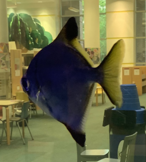
Figure 2-1. A fish!

Figure 2-2. Helvetica in a box
Traditional Challenges
How would you go about writing a program that could tell a fish from a cat? Maybe you’d write a set of rules describing that a cat has a tail, or that a fish has scales, and apply those rules to an image to determine what you’re looking at. But that would take time, effort, and skill. Plus, what happens if you encounter something like a Manx cat; while it is clearly a cat, it doesn’t have a tail.
You can see how these rules are just going get more and more complicated to describe all possible scenarios. Also, I’ll admit that I’m absolutely terrible at graphics programming, so the idea of having to manually code all these rules fills me with dread.
What we’re after is a function that, given the input of an image, returns cat or fish. That function is hard for us to construct by exhaustively listing all the criteria. But deep learning essentially makes the computer do all the hard work of constructing all those rules that we just talked about—provided we create a structure, give the network lots of data, and give it a way to work out whether it is getting the right answer. So that’s what we’re going to do. Along the way, you’ll learn some key concepts of how to use PyTorch.
But First, Data
First, we need data. How much data? Well, that depends. The idea that for any deep learning technique to work, you need vast quantities of data to train the neural network is not necessarily true, as you’ll see in Chapter 4. However, right now we’re going to be training from scratch, which often does require access to a large quantity of data. We need a lot of pictures of fish and cats.
Now, we could spend some time downloading many images from something like Google image search, but in this instance we have a shortcut: a standard collection of images used to train neural networks, called ImageNet. It contains more than 14 million images and 20,000 image categories. It’s the standard that all image classifiers judge themselves against. So I take images from there, though feel free to download other ones yourself if you prefer.
Along with the data, PyTorch needs a way to determine what is a cat and what is a fish. That’s easy enough for us, but it’s somewhat harder for the computer (which is why we are building the program in the first place!). We use a label attached to the data, and training in this manner is called supervised learning. (When you don’t have access to any labels, you have to use, perhaps unsurprisingly, unsupervised learning methods for training.)
Now, if we’re using ImageNet data, its labels aren’t going to be all that useful, because they contain too much information for us. A label of tabby cat or trout is, to the computer, separate from cat or fish. We’ll need to relabel these. Because ImageNet is such a vast collection of images, I have pulled together a list of image URLs and labels for both fish and cats.
You can run the download.py script in that directory, and it will download the images from the URLs and place them in the appropriate locations for training. The relabeling is simple; the script stores cat pictures in the directory train/cat and fish pictures in train/fish. If you’d prefer to not use the script for downloading, just create these directories and put the appropriate pictures in the right locations. We now have our data, but we need to get it into a format that PyTorch can understand.
PyTorch and Data Loaders
Loading and converting data into formats that are ready for training can often end up being one of the areas in data science that sucks up far too much of our time. PyTorch has developed standard conventions of interacting with data that make it fairly consistent to work with, whether you’re working with images, text, or audio.
The two main conventions of interacting with data are datasets and data loaders. A dataset is a Python class that allows us to get at the data we’re supplying to the neural network. A data loader is what feeds data from the dataset into the network. (This can encompass information such as, How many worker processes are feeding data into the network? or How many images are we passing in at once?)
Let’s look at the dataset first. Every dataset, no matter whether it includes images, audio, text, 3D landscapes, stock market information, or whatever, can interact with PyTorch if it satisfies this abstract Python class:
classDataset(object):def__getitem__(self,index):raiseNotImplementedErrordef__len__(self):raiseNotImplementedError
This is fairly straightforward: we have to implement a method that returns the size of our dataset (len), and implement a method that can retrieve an item from our dataset in a (label, tensor) pair. This is called by the data loader as it is pushing data into the neural network for training. So we have to write a body for getitem that can take an image and transform it into a tensor and return that and the label back so PyTorch can operate on it. This is fine, but you can imagine that this scenario comes up a lot, so maybe PyTorch can make things easier for us?
Building a Training Dataset
The torchvision package includes a class called ImageFolder that does pretty much everything for us, providing our images are in a structure where each directory is a label (e.g., all cats are in a directory called cat). For our cats and fish example, here’s what you need:
importtorchvisionfromtorchvisionimporttransformstrain_data_path="./train/"transforms=transforms.Compose([transforms.Resize(64),transforms.ToTensor(),transforms.Normalize(mean=[0.485,0.456,0.406],std=[0.229,0.224,0.225])])train_data=torchvision.datasets.ImageFolder(root=train_data_path,transform=transforms)
A little bit more is going on here because torchvision also allows you to specify a list of transforms that will be applied to an image before it gets fed into the neural network. The default transform is to take image data and turn it into a tensor (the transforms.ToTensor() method seen in the preceding code), but we’re also doing a couple of other things that might not seem obvious.
Firstly, GPUs are built to be fast at performing calculations that are a standard size. But we probably have an assortment of images at many resolutions. To increase our processing performance, we scale every incoming image to the same resolution of 64 × 64 via the Resize(64) transform. We then convert the images to a tensor, and finally, we normalize the tensor around a specific set of mean and standard deviation points.
Normalizing is important because a lot of multiplication will be happening as the input passes through the layers of the neural network; keeping the incoming values between 0 and 1 prevents the values from getting too large during the training phase (known as the exploding gradient problem). And that magic incarnation is just the mean and standard deviation of the ImageNet dataset as a whole. You could calculate it specifically for this fish and cat subset, but these values are decent enough. (If you were working on a completely different dataset, you’d have to calculate that mean and deviation, although many people just use these ImageNet constants and report acceptable results.)
The composable transforms also allow us to easily do things like image rotation and skewing for data augmentation, which we’ll come back to in Chapter 4.
Note
We’re resizing the images to 64 × 64 in this example. I’ve made that arbitrary choice in order to make the computation in our upcoming first network fast. Most existing architectures that you’ll see in Chapter 3 use 224 × 224 or 299 × 299 for their image inputs. In general, the larger the input size, the more data for the network to learn from. The flip side is that you can often fit a smaller batch of images within the GPU’s memory.
We’re not quite done with datasets yet. But why do we need more than just a training dataset?
Building Validation and Test Datasets
Our training data is set up, but we need to repeat the same steps for our validation data. What’s the difference here? One danger of deep learning (and all machine learning, in fact) is the concept of overfitting: your model gets really good at recognizing what it has been trained on, but cannot generalize to examples it hasn’t seen. So it sees a picture of a cat, and unless all other pictures of cats resemble that picture very closely, the model doesn’t think it’s a cat, despite it obviously being so. To prevent our network from doing this, we download a validation set in download.py, which is a series of cat and fish pictures that do not occur in the training set. At the end of each training cycle (also known as an epoch), we compare against this set to make sure our network isn’t getting things wrong. But don’t worry—the code for this is incredibly easy because it’s just the earlier code with a few variable names changed:
val_data_path="./val/"val_data=torchvision.datasets.ImageFolder(root=val_data_path,transform=transforms)
We just reused the transforms chain instead of having to define it once again.
In addition to a validation set, we should also create a test set. This is used to test the model after all training has been completed:
test_data_path="./test/"test_data=torchvision.datasets.ImageFolder(root=test_data_path,transform=transforms)
Distinguishing the types of sets can be a little confusing, so I’ve compiled a table to indicate which set is used for which part of model training; see Table 2-1.
Training set |
Used in the training pass to update the model |
Validation set |
Used to evaluate how the model is generalizing to the problem domain, rather than fitting to the training data; not used to update the model directly |
Test set |
A final dataset that provides a final evaluation of the model’s performance after training is complete |
We can then build our data loaders with a few more lines of Python:
batch_size=64train_data_loader=data.DataLoader(train_data,batch_size=batch_size)val_data_loader=data.DataLoader(val_data,batch_size=batch_size)test_data_loader=data.DataLoader(test_data,batch_size=batch_size)
The new thing to note from this code is batch_size. This tells us how many images will go through the network before we train and update it. We could, in theory, set the batch_size to the number of images in the test and training sets so the network sees every image before it updates. In practice, we tend not to do this because smaller batches (more commonly known as mini-batches in the literature) require less memory than having to store all the information about every image in the dataset, and the smaller batch size ends up making training faster as we’re updating our network much more quickly.
By default, PyTorch’s data loaders are set to a batch_size of 1. You will almost certainly want to change that. Although I’ve chosen 64 here, you might want to experiment to see how big of a minibatch you can use without exhausting your GPU’s memory. You may also want to experiment with some of the additional parameters: you can specify how datasets are sampled, whether the entire set is shuffled on each run, and how many worker processes are used to pull data out of the dataset. This can all be found in the PyTorch documentation.
That covers getting data into PyTorch, so let’s now introduce a simple neural network to actually start classifying our images.
Finally, a Neural Network!
We’re going to start with the simplest deep learning network: an input layer, which will work on the input tensors (our images); our output layer, which will be the size of the number of our output classes (2); and a hidden layer between them. In our first example, we’ll use fully connected layers. Figure 2-3 illustrates what that looks like with an input layer of three nodes, a hidden layer of three nodes, and our two-node output.

Figure 2-3. A simple neural network
As you can see, in this fully connected example, every node in a layer affects every node in the next layer, and each connection has a weight that determines the strength of the signal from that node going into the next layer. (It is these weights that will be updated when we train the network, normally from a random initialization.) As an input passes through the network, we (or PyTorch) can simply do a matrix multiplication of the weights and biases of that layer onto the input. Before feeding it into the next function, that result goes into an activation function, which is simply a way of inserting nonlinearity into our system.
Activation Functions
Activation functions sound complicated, but the most common activation function you’ll come across in the literature these days is ReLU, or rectified linear unit. Which again sounds complicated! But all it turns out to be is a function that implements max(0,x), so the result is 0 if the input is negative, or just the input (x) if x is positive. Simple!
Another activation function you’ll likely come across is softmax, which is a little more complicated mathematically. Basically it produces a set of values between 0 and 1 that adds up to 1 (probabilities!) and weights the values so it exaggerates differences—that is, it produces one result in a vector higher than everything else. You’ll often see it being used at the end of a classification network to ensure that that network makes a definite prediction about what class it thinks the input belongs to.
With all these building blocks in place, we can start to build our first neural network.
Creating a Network
Creating a network in PyTorch is a very Pythonic affair. We inherit from a class called torch.nn.Network and fill out the __init__ and forward methods:
classSimpleNet(nn.Module):def__init__(self):super(Net,self).__init__()self.fc1=nn.Linear(12288,84)self.fc2=nn.Linear(84,50)self.fc3=nn.Linear(50,2)defforward(self):x=x.view(-1,12288)x=F.relu(self.fc1(x))x=F.relu(self.fc2(x))x=F.softmax(self.fc3(x))returnxsimplenet=SimpleNet()
Again, this is not too complicated. We do any setup required in init(), in this case calling our superclass constructor and the three fully connected layers (called Linear in PyTorch, as opposed to Dense in Keras). The forward() method describes how data flows through the network in both training and making predictions (inference). First, we have to convert the 3D tensor (x and y plus three-channel color information—red, green, blue) in an image, remember!—into a 1D tensor so that it can be fed into the first Linear layer, and we do that using the view(). From there, you can see that we apply the layers and the activation functions in order, finally returning the softmax output to give us our prediction for that image.
The numbers in the hidden layers are somewhat arbitrary, with the exception of the output of the final layer, which is 2, matching up with our two classes of cat or fish. In general, you want the data in your layers to be compressed as it goes down the stack. If a layer is going to, say, 50 inputs to 100 outputs, then the network might learn by simply passing the 50 connections to 50 of the 100 outputs and consider its job done. By reducing the size of the output with respect to the input, we force that part of the network to learn a representation of the original input with fewer resources, which hopefully means that it extracts some features of the images that are important to the problem we’re trying to solve; for example, learning to spot a fin or a tail.
We have a prediction, and we can compare that with the actual label of the original image to see whether the prediction was correct. But we need some way of allowing PyTorch to quantify not just whether a prediction is right or wrong, but just how wrong or right it is. This is handled by a loss function.
Loss Functions
Loss functions are one of the key pieces of an effective deep learning solution. PyTorch uses loss functions to determine how it will update the network to reach the desired results.
Loss functions can be as complicated or as simple as you desire. PyTorch comes complete with a comprehensive collection of them that will cover most of the applications you’re likely to encounter, plus of course you can write your own if you have a very custom domain. In our case, we’re going to use a built-in loss function called CrossEntropyLoss, which is recommended for multiclass categorization tasks like we’re doing here. Another loss function you’re likely to come across is MSELoss, which is a standard mean squared loss that you might use when making a numerical prediction.
One thing to be aware of with CrossEntropyLoss is that it also incorporates softmax() as part of its operation, so our forward() method becomes the following:
defforward(self):# Convert to 1D vectorx=x.view(-1,12288)x=F.relu(self.fc1(x))x=F.relu(self.fc2(x))x=self.fc3(x)returnx
Now let’s look at how a neural network’s layers are updated during the training loop.
Optimizing
Training a network involves passing data through the network, using the loss function to determine the difference between the prediction and the actual label, and then using that information to update the weights of the network in an attempt to make the loss function return as small a loss as possible. To perform the updates on the neural network, we use an optimizer.
If we just had one weight, we could plot a graph of the loss value against the value of the weight, and it might look something like Figure 2-4.
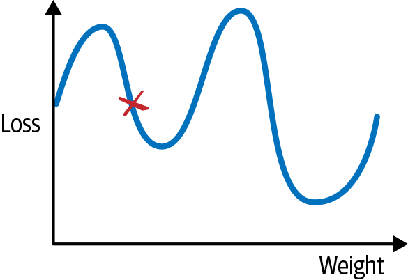
Figure 2-4. A 2D plot of loss
If we start at a random position, marked in Figure 2-4 by the X, with our weight value on the x-axis and the loss function on the y-axis, we need to get to the lowest point on the curve to find our optimal solution. We can move by altering the value of the weight, which will give us a new value for the loss function. To know how good a move we’re making, we can check against the gradient of the curve. One common way to visualize the optimizer is like rolling a marble, trying to find the lowest point (or minima) in a series of valleys. This is perhaps clearer if we extend our view to two parameters, creating a 3D graph as shown in Figure 2-5.
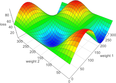
Figure 2-5. A 3D plot of loss
And in this case, at every point, we can check the gradients of all the potential moves and choose the one that moves us most down the hill.
You need to be aware of a couple of issues, though. The first is the danger of getting trapped in local minima, areas that look like they’re the shallowest parts of the loss curve if we check our gradients, but actually shallower areas exist elsewhere. If we go back to our 1D curve in Figure 2-4, we can see that if we end up in the minima on the left by taking short hops down, we’d never have any reason to leave that position. And if we took giant hops, we might find ourselves getting onto the path that leads to the actual lowest point, but because we keep making jumps that are so big, we keep bouncing all over the place.
The size of our hops is known as the learning rate, and is often the key parameter that needs to be tweaked in order to get your network learning properly and efficiently. You’ll see a way of determining a good learning rate in Chapter 4, but for now, you’ll be experimenting with different values: try something like 0.001 to begin with. As just mentioned, large learning rates will cause your network to bounce all over the place in training, and it will not converge on a good set of weights.
As for the local minima problem, we make a slight alteration to our taking all the possible gradients and indicate sample random gradients during a batch. Known as stochastic gradient descent (SGD), this is the traditional approach to optimizing neural networks and other machine learning techniques. But other optimizers are available, and indeed for deep learning, preferable. PyTorch ships with SGD and others such as AdaGrad and RMSProp, as well as Adam, the optimizer we will be using for the majority of the book.
One of the key improvements that Adam makes (as does RMSProp and AdaGrad) is that it uses a learning rate per parameter, and adapts that learning rate depending on the rate of change of those parameters. It keeps an exponentially decaying list of gradients and the square of those gradients and uses those to scale the global learning rate that Adam is working with. Adam has been empirically shown to outperform most other optimizers in deep learning networks, but you can swap out Adam for SGD or RMSProp or another optimizer to see if using a different technique yields faster and better training for your particular application.
Creating an Adam-based optimizer is simple. We call optim.Adam() and pass in the weights of the network that it will be updating (obtained via simplenet.parameters()) and our example learning rate of 0.001:
importtorch.optimasoptimoptimizer=optim.Adam(simplenet.parameters(),lr=0.001)
The optimizer is the last piece of the puzzle, so we can finally start training our network.
Training
Here’s our complete training loop, which combines everything you’ve seen so far to train the network. We’re going to write this as a function so parts such as the loss function and optimizer can be passed in as parameters. It looks quite generic at this point:
forepochinrange(epochs):forbatchintrain_loader:optimizer.zero_grad()input,target=batchoutput=model(input)loss=loss_fn(output,target)loss.backward()optimizer.step()
It’s fairly straightforward, but you should note a few things. We take a batch from our training set on every iteration of the loop, which is handled by our data loader. We then run those through our model and compute the loss from the expected output. To compute the gradients, we call the backward() method on the model. The optimizer.step() method uses those gradients afterward to perform the adjustment of the weights that we talked about in the previous section.
What is that zero_grad() call doing, though? It turns out that the calculated gradients accumulate by default, meaning that if we didn’t zero the gradients at the end of the batch’s iteration, the next batch would have to deal with this batch’s gradients as well as its own, and the batch after that would have to cope with the previous two, and so on. This isn’t helpful, as we want to look at only the gradients of the current batch for our optimization in each iteration. We use zero_grad() to make sure they are reset to zero after we’re done with our loop.
That’s the abstracted version of the training loop, but we have to address a few more things before we can write our complete function.
Making It Work on the GPU
If you’ve run any of the code so far, you might have noticed that it’s not all that fast. What about that shiny GPU that’s sitting attached to our instance in the cloud (or the very expensive machine we’ve put together on our desktop)? PyTorch, by default, does CPU-based calculations. To take advantage of the GPU, we need to move our input tensors and the model itself to the GPU by explicitly using the to() method. Here’s an example that copies the SimpleNet to the GPU:
iftorch.cuda.is_available():device=torch.device("cuda")elsedevice=torch.device("cpu")model.to(device)
Here, we copy the model to the GPU if PyTorch reports that one is available, or otherwise keep the model on the CPU. By using this construction, we can determine whether a GPU is available at the start of our code and use tensor|model.to(device) throughout the rest of the program, being confident that it will go to the correct place.
Note
In earlier versions of PyTorch, you would use the cuda() method to copy data to the GPU instead. If you come across that method when looking at other people’s code, just be aware that it’s doing the same thing as to()!
And that wraps up all the steps required for training. We’re almost done!
Putting It All Together
You’ve seen a lot of different pieces of code throughout this chapter, so let’s consolidate it. We put it all together to create a generic training method that takes in a model, as well as training and validation data, along with learning rate and batch size options, and performs training on that model. We use this code throughout the rest of the book:
deftrain(model,optimizer,loss_fn,train_loader,val_loader,epochs=20,device="cpu"):forepochinrange(epochs):training_loss=0.0valid_loss=0.0model.train()forbatchintrain_loader:optimizer.zero_grad()inputs,target=batchinputs=inputs.to(device)target=targets.to(device)output=model(inputs)loss=loss_fn(output,target)loss.backward()optimizer.step()training_loss+=loss.data.item()training_loss/=len(train_iterator)model.eval()num_correct=0num_examples=0forbatchinval_loader:inputs,targets=batchinputs=inputs.to(device)output=model(inputs)targets=targets.to(device)loss=loss_fn(output,targets)valid_loss+=loss.data.item()correct=torch.eq(torch.max(F.softmax(output),dim=1)[1],target).view(-1)num_correct+=torch.sum(correct).item()num_examples+=correct.shape[0]valid_loss/=len(valid_iterator)('Epoch:{}, Training Loss:{:.2f},ValidationLoss:{:.2f},accuracy={:.2f}'.format(epoch, training_loss,valid_loss,num_correct/num_examples))
That’s our training function, and we can kick off training by calling it with the required parameters:
train(simplenet,optimizer,torch.nn.CrossEntropyLoss(),train_data_loader,test_data_loader,device)
The network will train for 20 epochs (you can adjust this by passing in a value for epoch to train()), and you should get a printout of the model’s accuracy on the validation set at the end of each epoch.
You have trained your first neural network—congratulations! You can now use it to make predictions, so let’s look at how to do that.
Making Predictions
Way back at the start of the chapter, I said we would make a neural network that could classify whether an image is a cat or a fish. We’ve now trained one to do just that, but how do we use it to generate a prediction for a single image? Here’s a quick bit of Python code that will load an image from the filesystem and print out whether our network says cat or fish:
fromPILimportImagelabels=['cat','fish']img=Image.open(FILENAME)img=transforms(img)img=img.unsqueeze(0)prediction=simplenet(img)prediction=prediction.argmax()(labels[prediction])
Most of this code is straightforward; we reuse the transform pipeline we made earlier to convert the image into the correct form for our neural network. However, because our network uses batches, it actually expects a 4D tensor, with the first dimension denoting the different images within a batch. We don’t have a batch, but we can create a batch of length 1 by using unsqueeze(0), which adds a new dimension at the front of our tensor.
Getting predictions is as simple as passing our batch into the model. We then have to find out the class with the higher probability. In this case, we could simply convert the tensor to an array and compare the two elements, but there are often many more than that. Helpfully, PyTorch provides the argmax() function, which returns the index of the highest value of the tensor. We then use that to index into our labels array and print out our prediction. As an exercise, use the preceding code as a basis to work out predictions on the test set that we created at the start of the chapter. You don’t need to use unsqueeze() because you get batches from the test_data_loader.
That’s about all you need to know about making predictions for now; we return to this in Chapter 8 when we harden things for production usage.
In addition to making predictions, we probably would like to be able to reload the model at any point in the future with our trained parameters, so let’s take a look at how that’s done with PyTorch.
Model Saving
If you’re happy with the performance of a model or need to stop for any reason, you can save the current state of a model in Python’s pickle format by using the torch.save() method. Conversely, you can load a previously saved iteration of a model by using the torch.load() method.
Saving our current parameters and model structure would therefore work like this:
torch.save(simplenet,"/tmp/simplenet")
And we can reload as follows:
simplenet=torch.load("/tmp/simplenet")
This stores both the parameters and the structure of the model to a file. This might be a problem if you change the structure of the model at a later point. For this reason, it’s more common to save a model’s state_dict instead. This is a standard Python dict that contains the maps of each layer’s parameters in the model. Saving the state_dict looks like this:
torch.save(model.state_dict(),PATH)
To restore, create an instance of the model first and then use load_state_dict. For SimpleNet:
simplenet=SimpleNet()simplenet_state_dict=torch.load("/tmp/simplenet")simplenet.load_state_dict(simplenet_state_dict)
The benefit here is that if you extend the model in some fashion, you can supply a strict=False parameter to load_state_dict that assigns parameters to layers in the model that do exist in the state_dict, but does not fail if the loaded state_dict has layers missing or added from the model’s current structure. Because it’s just a normal Python dict, you can change the key names to fit your model, which can be handy if you are pulling in parameters from a completely different model altogether.
Models can be saved to a disk during a training run and reloaded at another point so that training can continue where you left off. That is quite useful when using something like Google Colab, which lets you have continuous access to a GPU for only around 12 hours. By keeping track of time, you can save the model before the cutoff and continue training in a new 12-hour session.
Conclusion
You’ve taken a whirlwind tour through the basics of neural networks and learned how, using PyTorch, you can train them with a dataset, make predictions on other images, and save/restore models to and from disk.
Before you read the next chapter, experiment with the SimpleNet architecture we created here. Adjust the number of parameters in the Linear layers, and maybe add another layer or two. Have a look at the various activation functions available in PyTorch and swap out ReLU for something else. See what happens to training if you adjust the learning rate or switch out the optimizer from Adam to another option (perhaps try vanilla SGD). Maybe alter the batch size and the initial size of the image as it gets turned into a 1D tensor at the start of the forward pass. A lot of deep learning work is still in the phase of artisanal construction; learning rates are tinkered with by hand until a network is trained appropriately, so it’s good to get a handle on how all the moving parts interact.
You might be a little disappointed with the accuracy of the SimpleNet architecture, but don’t worry! Chapter 3 provides some definite improvements as we introduce the convolutional neural network in place of the very simple network we’ve been using so far.
Further Reading
-
“Adam: A Method for Stochastic Optimization” by Diederik P. Kingma and Jimmy Ba (2014)
-
“An Overview of Gradient Descent Optimization Algorithms” by Sebstian Ruder (2016)