Chapter 1. Reductions in Spark
The focus of this chapter is to present the concept of reduction transformations in Spark. Typically, a reduction is over a set of values per key. Most of data algorithms and ETL require reduction of values by some keys (such as finding mean and median over a set of stock values). This chapter covers
-
Reduction concepts
-
What is a monoid?
-
Reductions in Spark
-
Most important Spark reduction transformations:
-
reduceByKey() -
combineBykey() -
groupBykey() -
aggregateByKey() -
sortByKey()
-
The main goal of this chapter is to
present reduction transformations on
Resilient Distributed Datasets (RDDs).
This chapter covers how to work with pair
RDDs of (key, value) pairs, which are a
common data abstraction required for many
operations in Spark. Pair RDDs are commonly
used to perform aggregations (sum, average,
median, T-test, …), and often we will do
some initial ETL (extract, transform, and
load) to get our data into a `(key, value)
form. With pair RDDs you may perform any
desired aggregation over a set of values.
Spark supports powerfull reducer
transformations and actions. All
reducers by keys are denoted by
<reducer_name>ByKey()
transformations, which accepts a source
RDD[(K, V)] and creates a target
RDD[(K, C)] (for some transformations
such as reduceByKey(), the V and C
are the same. The function of
<reducer_name>ByKey() transformation
is to reduce all values of a given key
(for all unique keys).
The reduction by key can be simply
-
An average of all values
-
Sum and count of all values
-
Mode and median of all values
-
Standard deviation of all values
-
T-test of all values
For some of the reduction operations
(such as median — which is the “middle”
of a sorted list of numbers), you do
need all values at the same time before
finding the median. But for some other
functions, such as sum and count of all
values, the reducer does not need all
values at the same time. For example,
if you want to find the median of all
values, then groupByKey() will be a
good choice, but this transformation
does not do well if a key has lots of
values (which might cause an OOM problem).
On the otherhand if you want to find the
sum and count of all values, then the
reduceByKey() will be a good choice,
which merges the values for each key
using an associative and commutative
reduce function.
The purpose of this chapter is to show the most important Spark’s reduction transformations by simple working PySpark examples. Spark has many reduction transformations, but we will focus on the transformations used by most of the Spark applications.
Since pair RDDs are required for reducer transormations by keys, next I present creating pair RDDs.
Creating Pair RDDs
Given a set of keys and their associated
values, a reduction transformation is a
transformation to reduce values of each
key using an algorithm (sum of value,
median of values, …). The reduction
transformations presented in this chapter
will work on (key, value) pairs. This
means that RDD elements must conform to
(key, value) pairs. There are several
ways to create pair RDDs in Spark. The
simple way to way create pair RDDs is
by a map() function that returns
(key, value) pairs. Also, to create a
set of (key, value) pairs, you may use
parallelize() on collections (such
as list of tupes and dictionaries).
To perform any reductions by keys (such
as reduceByKey(), groupByKey(), …),
your RDD must be a pair RDD, where each
element is a (key, value) pair.
Example: Using Collections
You may use Python’s collections to create pair RDDs. The following illustrates how to create pair RDDs:
>>>key_value=[('A',2),('A',4),('B',5),('B',7)]>>>pair_rdd=spark.sparkContext.parallelize(key_value)>>>pair_rdd.collect()[('A',2),('A',4),('B',5),('B',7)]>>>pair_rdd.count()4>>>hashmap=pair_rdd.collectAsMap()>>>hashmap{'A':4,'B':7}

pair_rddhas two keys as{'A', 'B'}
Example: Using map() Transformation
Suppose you have weather-related data and you
want to create pairs of (city_id, temprature).
Assume that you input has the following format:
<city_id><,><lattitude><,><longtitue><,>temprature>
With a map() transformation and a simple
Pythn function, you can create your desired
pair RDD.
-
Create a function to create (key, value) pair
defcreate_key_value(rec):tokens=rec.split(",")city_id=tokens[0]temprature=tokens[3]return(city_id,temprature)
key is
city_idand value istemprature-
Use
map()to create pair RDD:
-
input_path=<your-temprature-data-path>rdd=spark.sparkContext.textFile(input_path)pair_rdd=rdd.map(create_key_value)# or we may write it using lambda aspair_rdd=rdd.map(lambdarec:create_key_value(rec))
The are many other ways to create (key, value)
pair RDDs: such as map(), reduceByKey(), combineByKey(), etc. For example,
reduceByKey() accepts a source RDD of (K, V)
and produces a target RDD of (K, V). On the
otherhand combineByKey() accepts a source RDD of
(K, V) and produces a target RDD of (K, C)
where V and C can be different data types
(if desired).
Reducer transformations
Typically, a reducer transformation reduces the data size from a larger batch of values (such as list of numbers) to a smaller one (such as sum, median, or average of the list of numbers). An example of a reducer by key can be:
-
find sum and average of all values
-
find mean, mode and median of all values
-
calculate mean and standard deviation of all values
-
find (min, max, count) for all values
-
find Top-10 of all values
In a nutshell, the reduce transformation roughly corresponds to the fold operation (also termed reduce, accumulate, aggregate) in functional programming. Reducer transformations are either applied to all data elements (such as finding sum of all elements) or to all elements per key (such as finding sum of all elements per key).
A simple addition reduction over a set
of numbers {47, 11, 42, 13} for a single
partition is illustrated in Figure 4.1.

Figure 1-1. Reduction Concept
Another addition reduction concept is
illustrated by the Figure 4.2. This is
a reduction, which adds the elements of
2 partitions (note that Spark manages
data using partitions — called chunks — that helps parallelize distributed data
processing with minimal network traffic
for sending data between executors).
The final reduced values for Partition-1
and Partition-2 are 21 and 18. Each
partition performs local reductions and
finally the result of two partitions are
reduced.

Figure 1-2. Reduction Concept
Reducer is a core concept in functional
programming, which reduces a set of objects
(such as numbers, strings, lists, …) into
a single value (such as sum of numbers,
concatenation of string objects). Spark and
MapReduce paradigm use the reducer concept
to aggregate a set of values into a single
value for a given set of keys. In the
simplest form consider the following
(key, value) pairs (where key is a
String and value is a list of Integers)
(key1, [1, 2, 3])
(key2, [40, 50, 60, 70, 80])
(key3, [8])
The most simple reducer will be an addition function over a set of values per key. Once we apply the addition reducer, the result will be:
(key1, 6)
(key2, 300)
(key3, 8)
Or you may reduce each (key, value)
to (key, pair) where pair is
(sum-of-values, count-of-values):
(key1, (6, 3))
(key2, (300, 5))
(key3, (8, 1))
Reducers are designed to operate concurrently and independently: meaning that there is no synchronization between reducers. The more resources a Spark cluster has, reductions can be done faster. In the worst possible case, if we have only one reducer, then reduction will work as a queue operation. In general, a cluster will offer many reducers (depending on the resource availability) for the reduction transformation.
In MapReduce programming paradigm,
the programmer defines a mapper and
a reducer with the following map()
and reduce() signatures:
-
map: (K~1~, V~1~) -> [(K~2~, V~2~)] -
reduce: (K~2~, [V~2~]) -> [(K~3~, V~3~)]
The map() function maps a
(key~1~, value~1~) pair into
a set of (key~2~, value~2~)
pairs. After all maps are
completed, the sort and shuffle
automatically is done (provided
by the MapReduce paradigm and
not done by the programmer). The
the sort and shuffle phase of
MapReduce paradigm is very similar
to the Spark’s groupByKey()
transformation
The reduce() function reduces a
(key~2~, [value~2~]) pair into
a set of (key~3~, value~3~)
pairs
The convention [...] is used
to denote a list of objects (or
an iterable list of objects).
Therefore, we can say that a reducer
transformation takes a list of values
and reduces it to a tangible result
(such as sum of values, average of
values, or your desired data
structure).
In MapReduce and distributed algorithms,
reduction (the so called reduce() function)
step is a required operation in solving
a problem. Spark provides an easy to
use rich set of reduction transformations.
Throught the chapter we’ll discuss
Spark’s reduction transformations
(such as reduceByKey(),
groupByKey(), aggregateByKey(), and
combineByKey()) on a given list of
(key, value) pairs, typically emitted
by mappers or generated by an ETL program.
In general, the combineByKey() is more
general than reduceByKey() and
aggregateByKey().
The groupByKey() transformation is
very simple to use and its reduction
transformation concept is illustrated
by the Figure 4.3. In this example,
we have four unique keys {A, B, C, P }
and their associated values are grouped
as a list of integers. In this example,
-
Source RDD:
-
RDD[(String, Integer)] -
Each element is a pair of
(String, Integer)
-
-
Target RDD:
-
RDD[(String, [Integer])] -
Each element is a pair of
(String, [Integer]), where value is a list/iterable of integers.
-
Informally and in a nutshell, Spark’s
groupByKey() transformation works very
similar to the SQL’s GROUP BY statement.

Figure 1-3. The groupByKey() transformation example
You should note that, by default,
Spark reductions do not sort the
reduced values. For example looking
at Figure 3, the reduced value for
key B can be [4, 8] or [8, 4].
If desired, you may sort the values
before the final reduction. Therefore,
if your reduction algorithm requires
sorting, then you should sort values
explicityly.
Next, we focus on Spark’s reduction transformations on RDDs. In general most of the Spark applications will require several reductions by keys
Spark’s Reductions
Spark is a fast and general engine
for large scale data processing.
Spark provides a high-level MapReduce
API (such as map() and reduce())
and beyond (such as filter() and
many other useful reduction by key
transformations). Indeed,
Spark’s API is a superset (by providing
natural join and merge functionalities)
of Hadoop’s classic MapReduce API.
Spark’s operations (transformations and
actions) is much more powerful, higher
level, easy to use, and faster than
Hadoop’s classic MapReduce paradigm.
According to Spark documentation, you
may run Spark programs up to 100x faster
than Hadoop MapReduce in memory, or
10x faster on disk. In summary, Spark
is easier, richer, and faster than
Hadoop’s classic MapReduce programming
model. The API in this chapter is
based on Spark-3.0.0.
Spark offers a set of high-level and powerful by key reducers. Some of the most important and common reducers are listed in Table 1.
| Transformation | Purpose |
|---|---|
|
Combine values with the same key |
|
Group values with the same key |
|
Aggregate the values of each key, using given combine functions and a neutral “zero value”. |
|
Generic function to combine the elements for each key using a custom set of aggregation functions. |
We will discuss these reduction transformations in the context of PySpark examples.
Internally , the aggregateByKey(),
reduceByKey() and groupByKey()
are implemented by combineByKey().
The aggregateByKey() transformation
is similar to reduceByKey() but
you can provide initial values (per
partition) when performing aggregation.
Using reduceByKey() will provide the
most optimized performance (without
writing 3 additional functions — create_combiner, merge_value,
merge_combiners — that you have
to provide for the combineByKey()).
If you can not (such as when the input
and result types differ from each other)
use reduceByKey(), then consider
using combineByKey(), which
you have to provide 3 additional small
functions.
Finally, if solving the group-by-key
aggregation by reduceByKey() or
combineByKey() is very hard and
complex, then you may use the groupByKey().
While the use of combineByKey() takes a
little more work than using a groupByKey()
call, but avoiding groupByKey() can improve
your spark job performance by reducing the
amount of data sent across the network.
If you are going to use groupByKey(),
then make sure that you have enough memory
in your cluster to handle all of values per
key. When possible, use combineByKey()
or reduceByKey() transformation to
reduce the amount of shuffle data.
What is a Reduction?
According to a couple of dictionaries: reduction is defined as:
-
the act of making something smaller in size, amount, number, etc.
-
the act of reducing something
-
an amount by which something is reduced
-
the act or process of reducing : the state of being reduced
-
the action or fact of making a specified thing smaller or less in amount, degree, or size.
-
the process of converting an amount from one denomination to a smaller one, or of bringing down a fraction to its lowest terms.
Our focus will be on reductions, where the source
RDD is of the form RDD[(K, V)] (an RDD where
elements are pairs of (K, V) — this is called
a pair RDD). In Spark and MapReduce paradigm,
the reduction is the process of applying some
function f() on the values (V~1~, V~2~, ...,
V~n~) for every key K in the RDD[(K, V)]
(called a pair RDD). The function f() can be
something as trivial as summation of the values
or can be as complex as your requirement.
Therefore, we will assume that each RDD has a
set of keys and for each key (such as K) we
have a set of values as illustrated below.
{ (K, V~1~), (K, V~2~), ..., (K, V~n~) }
Of course this a simplistic view of a reducer.
In real applications, values for the same key
(here denoted as K) can come from many different
partitions and each partition can come from a
different server. Note that there is no order
(such as ascending or descending) between the
values
{ V~1~, V~2~, ..., V~n~ }
for a given key K. In Spark, based on
your selected transformation (such as
groupByKey(), reduceByKey(), or
combineByKey()) sort and shuffle phase
can be done very differently, which might
have a different efficiency and scale-out.
Spark’s Reduction Transformations
Spark (Table 1.2) provides the following
<reduction-name>ByKey() transformation
functions over a set of (key, value) pairs
(partial listing):
| Reduction Transformation | Description |
|---|---|
|
Group the values for each key in the RDD into a single sequence |
|
Merge the values for each key using an associative and commutative reduce function |
|
Generic function to combine the elements for each key using a custom set of aggregation functions |
|
Aggregate the values of each key, using given combine functions and a neutral “zero value” |
|
Merge the values for each key using an associative function and a neutral “zero value” …) |
|
Count the number of elements for each key, and return the result to the master as a Map |
|
Return a subset of this RDD sampled by key (via stratified sampling) |
|
Sort the RDD by key, so that each partition contains a sorted range of the elements in ascending order |
|
Return an RDD with the pairs from |
These group of transformation functions
act on (key, value) pairs represented
by RDDs. For example, in Java
programming language, (key, value)
pairs are represented by
JavaPairRDD<K,V>, but since Python
is a type-less language, (key, value)
pairs are represented as (key, value),
which is a tuple of 2 elements.
Therefore, Spark provides several ways
to do reductions on data. Here, I will
discuss the performance of each reduction
function with respect to the size of
values per given unique key. It has
been well documented that, for example,
the performance of Spark’s reduceByKey()
is much better than groupByKey()
when aggregation or reduction is done
over a lot of values per given key.
In this chapter, we will look only into
reductions of data over a set of given
unique keys. For example, given the
following (key, value) pairs for key=K:
{ (K, V~1~), (K, V~2~), ..., (K, V~n~)}
We are assuming that the key K has a list
of n ( n > 0 ) values:
[V~1~, V~2~, ..., V~n~]
To keep it simple, the goal of reduction
is to generate the following pair (or a
set of new (key, value) pairs):
(K, R)
where
f(V~1~, V~2~, ..., V~n~) -> R
where the function f() is called a
reducer or reduction function.
Spark provides a set of transformations
(such as groupByKey(), reduceByKey(),
combineByKey(), aggregateByKey(),
…) to apply function f() over a
list of values: [V~1~, V~2~, ..., V~n~].
To find the educed value, R, we have
many options in Spark, but the performance
and scalability of these transformation
will differ based on the number of values
processed over a set of keys. Spark does
not impose any ordering among the values
([V~1~, V~2~, ..., V~n~]) to be reduced.
Simple Warmup Example
Suppose we have a list of pairs: (K, V)
where K (as a key) is a String and V (as
a value) is an Integer number:
[
 ('alex', 2), ('alex', 4), ('alex', 8),
 ('jane', 3), ('jane', 7),
 ('rafa', 1), ('rafa', 3), ('rafa', 5), ('rafa', 6),
 ('clint', 9)
]
In this example, we have 4 unique keys:
{ 'alex', 'jane', 'rafa', 'clint' }
Suppose we want to combine (add the values) the values per key. The result of this reduction will be:
[
 ('alex', 14),
 ('jane', 10),
 ('rafa', 15),
 ('clint', 9)
]
where
  key: alex =>    14 = 2+4+8
  key: jane =>    10 = 3+7
  key: rafa =>    15 = 1+3+5+6
  key: clint =>    9 (single value, no operation is done)
There are so many ways to add these numbers to get the desired result. How did we arrive with these reduced (key, value) pairs? For this example, we may use any of the Spark transformations. Aggregating the values per key or combining the values per key is a reduction function. In classic MapReduce paradigm, this is called a “reduce by key” (or simply reduce) function. The MapReduce’s framework calls the application’s (user defined) “reduce” function once for each unique key in the sorted order of keys. The “reduce” function can iterate through the values that are associated with that key and produce zero or more outputs as (key, value) pairs. The “reduce” function solves the problem of combining the elements of each unique key to a single value. Note that in some applications, the result might be more than a single value.
Here I present 4 different solutions using
Spark’s transformations. For all solutions,
we will use the following Python data and
key_value_pairs (as RDD[(String, Integer)]),
which represents a set of (key=String,
value=Integer) pairs.
>>>data=[('alex',2),('alex',4),('alex',8),('jane',3),('jane',7),('rafa',1),('rafa',3),('rafa',5),('rafa',6),('clint',9)]>>>>>>key_value_pairs=spark.SparkContext.parallelize(data)>>>key_value_pairs.collect()[('alex',2),('alex',4),('alex',8),('jane',3),('jane',7),('rafa',1),('rafa',3),('rafa',5),('rafa',6),('clint',9)]
Python collection: list of pairs

key_value_pairsis anRDD[(String, Integer)]
Solution by reduceByKey()
Adding values for a given key is pretty
straightforward. Add every 2 values and
keep going. This is the most efficient
solution since combiners are used at worker
levels and finally the partition values are
added. A reducing addition (+) function
is an associative binary operation. The
source and target RDDs for reduceByKey()
transformation can be stated as:
source RDD: RDD[(K, V)]
target RDD: RDD[(K, V))
Note that source and target data types of
RDD values (V) are the same (this is a
limitation on the reduceByKey() — this
limitation can be removed by using the
combineByKey() or aggregateByKey()).
Using Lambda Expressions
This solution uses reduceByKey() and Lambda
Expressions (anonymous function):
# a is (an accumulated) value for key=K# b is a value for key=Ksum_per_key=key_value_pairs.reduceByKey(lambdaa,b:a+b)sum_per_key.collect()[('jane',10),('rafa',15),('alex',14),('clint',9)]
Using Functions
Instead of using Lambda Expressions, you may
use a defined function, such as add:
fromoperatorimportaddsum_per_key=key_value_pairs.reduceByKey(add)sum_per_key.collect()[('jane',10),('rafa',15),('alex',14),('clint',9)]
Adding values per key by reduceByKey() is
an optimized solution, since aggregation will
happen in all partitions before final aggregation
of the all partitions. According to Spark:
reduceByKey() merges the values for each key
using an associative and commutative reduce
function. This means that combiners (optimized
mini-reducers) are used in all cluster nodes
before merging the values per partitions.
Solution by groupByKey()
We can solve this problem by using the groupByKey()
transformation, but this solution will not have an
ideal performance since we will move lots of data to
the reducer nodes.
sum_per_key=key_value_pairs.grouByKey().mapValues(lambdavalues:sum(values))sum_per_key.collect()[('jane',10),('rafa',15),('alex',14),('clint',9)]
Group values (similar to SQL’s
GROUP BY) per key, now each key will have a set of Integer values; for example these three pairs{('alex', 2), ('alex', 4), ('alex', 8)}will be reduced to a single pair of('alex', [2, 4, 8])Add values per key using Python’s sum() function
The source and target RDDs for groupByKey()
transformation can be stated as:
source RDD: RDD[(K, V)]
Value is a type
VValue is an iterable/list of
Vas[V]
Note that source and target data types are not
the same. The value data type for source RDD
is V, while the the value data type for taget
RDD is [V] (as a iterable/list of V — denoted as [V]).
Solution by aggregateByKey()
In simplest form, the aggregateByKey()
transformation is defined as:
aggregateByKey(zero_value, seq_func, comb_func)

source RDD: RDD[(K, V)]
target RDD: RDD[(K, C))

V and C can be different data types.
According to Spark: aggregateByKey()
aggregates the values of each key, using
given combine functions and a neutral
“zero value”. This function can return
a different result type, C, than the
type of the values in the source RDD,
V. Thus, we need one operation
for merging a V into a C (per partition)
and one operation for merging two C’s
(merging values of two partitions) into a
single C. The former operation is used for
merging values within a single partition,
and the latter is used for merging values
between partitions. To avoid memory
allocation, both of these functions
are allowed to modify and return their
first argument instead of creating a
new C. Note that C and V can be
different data types. For this example both
are Integer data types.
Sum of values is presented by using
the aggregateByKey() transformation:
# zero_value -> C# seq_func: (C, V) -> C# comb_func: (C, C) -> C#>>>sum_per_key=key_value_pairs.aggregateByKey(...0,...(lambdaC,V:C+V),...(lambdaC1,C2:C1+C2)...)>>>sum_per_key.collect()[('jane',10),('rafa',15),('alex',14),('clint',9)]>>>
zero_value: initial value, applied per partitionseq_func: used on single partition
comb_func: combining values of partitions
Solution by combineByKey()
The combineByKey() transformation is the
most general and powerful among all reduce
by key transformations. In its simplest form,
the combineByKey() transformation is defined
as:
combineByKey(create_combiner, merge_value, merge_combiners)

source RDD: RDD[(K, V)]
target RDD: RDD[(K, C))

V and C can be different data types.

Generic function to combine the elements for each
key using a custom set of aggregation functions.
The combineByKey() transformation turns an
RDD[(K, V)] into a result of type RDD[(K, C)],
for a “combined type” C. Note that V and C
can be different data types (this is the power
of combineByKey()), but for this example,
both are Integer data types.
The combineByKey() interface allows you
to customize combining behavior. This
transformation enable us to create a custome
combined data type C as well as customizing
the reduction and combining behavior.
To use this transformation, we have to provide three functions:
-
create_combiner, which turns a singleVinto aC(e.g., creates a one-element list). This is used within a single partition to initialize aC. -
merge_value, to merge aVinto aC(e.g., adds it to the end of a list). This is used within a single partition to aggregate values into aC. -
merge_combiners, to combine twoC’s into a singleC(e.g., merges the lists). This is used in merging values from two partitions.
>>>sum_per_key=key_value_pairs.combineByKey(...(lambdav:v),...(lambdaC,v:C+v),...(lambdaC1,C2:C1+C2)...)>>>sum_per_key.collect()[('jane',10),('rafa',15),('alex',14),('clint',9)]
create_combiner: initial value per partitionmerge_value: used on single partitionsmerge_combiners: combine partitions into final result
Overall, the combineByKey() transformation
is the most powerful reduction in Spark, since
the data type of values (V) of source RDD can
be different from the data type of values (C)
of target RDD. For example, reduceByKey()
is a very special case of combineByKey():
V and C are the same data types. For
example, using combineByKey(), V can be
an Integer data type, while C can be a
pair of (Float, Integer) or other composite
data types.
To see the real power of the combineByKey()
transformation, lets find mean of values
per key. To solve this, we create a combined
data type (C) as (sum, count), which will
hold the sum of values and their associated
count:
# C = combined type as (sum, count)>>>sum_count_per_key=key_value_pairs.combineByKey(...(lambdav:(v,1)),...(lambdaC,v:(C[0]+v,C[1]+1),...(lambdaC1,C2:(C1[0]+C2[0],C1[1]+C2[1]))...)>>>mean_per_key=sum_count_per_key.mapValues(lambdaC:C[0]/C[1])
Given 3 partitions named {P1, P2, P3},
the following figure shows how to create a
Combiner (data type C), how to Merge a
value into a Combiner, and finally how to
merge two combiners.

Figure 1-4. The combineByKey() transformation example
Next, I will discuss the concept of a Monoid, which will help us to understand the concept of combiners in reduction transformations.
What is a Monoid?
Since Spark’s reductions execute on a partition by partition basis (i.e., your reducer function is distributed rather than being a sequential function), you need to make sure that your reducer function is semantically correct. To write proper reducers, which will generate correct output and results, we do need to understand the concept of a monoid. When reducing values, if your reducer function is not a monoid, then your final result will not be a correct value. This will be demonstrated shortly. In a nutshell, we can say that reducers are morphisms of monoids. The first step in creating a proper reducer is to identify the monoid. I will define monoid and provide some related examples shortly.
In algebra, a monoid is an algebraic
structure with a single associative
binary operation and an identity element
(also called a Zero element). For our
purposes, I will provide an informal
definition of a monoid:
M = (T, f, Zero) is a monoid, where
-
Tis a data type -
f()is a binary operation:f: (T, T) -> T -
Zero: T(an instance ofT)
The Zero is an identity (neutral) element of
type T and does not necessarily mean number zero.
With the properties specified below, the triple
(T, f, Zero) is called a monoid. Here are the
monoidic properties:
Let a, b, c, Zero be type of T
Then the following properties must hold:
-
Binary operation:
f: (T, T) -> T
-
Neutral element:
for all a in T:

f(Zero, a) = a
f(a, Zero) = a
-
Associativity:
for all a, b, c in T:

f(f(a, b), c) = f(a, f(b, c))
Not every binary operation in the world
is a monoid. For example, the mean (average
of numbers over a set of Integers) function
is not a monoid and the proof is given below.
Below we prove that the mean() is not an
associative function and therefore it is not
a monoid.
mean(10, mean(30, 50)) != mean(mean(10, 30), 50)

where

   mean(10, mean(30, 50))
      = mean (10, 40)
      = 25

   mean(mean(10, 30), 50)
      = mean (20, 50)
      = 35

   25 != 35
Therefore, mean() function over a set of Integers
is not a monoid. Let’s look at some examples.
Monoid Examples
To help you understand monoids, here are some monoid examples:
-
Integers with addition:
   ((a + b ) + c) = (a + (b + c))
   0 + n = n
   n + 0 = n
   The Zero element for addition is number 0.
-
Integers with multiplication:
   ((a * b) * c) = (a * (b * c))
   1 * n = n
   n * 1 = n
   The Zero element for multiplication is number 1.
-
Strings with concatenation:
   (a + (b + c)) = ((a + b) + c)
   "" + s = s
   s + "" = s
   The Zero element for concatenation is an empty string of size 0.
-
Lists with concatenation:
List(a, b) + List(c, d) = List(a,b,c,d)
-
Sets with their union:
   Set(1,2,3) + Set(2,4,5)
      = Set(1,2,3,2,4,5)
      = Set(1,2,3,4,5)

   S + {} = S
   {} + S = S
   The Zero element is an empty set {}.
Non-Monoid Examples
Here are some non-monoid examples:
-
Integers with mean function:
mean(mean(a,b),c) != mean(a, mean(b,c))
-
Integers with subtraction:
((a - b) -c) != (a - (b - c))
-
Integers with division:
((a / b) / c) != (a / (b / c))
-
Integers with mode:
mode(mode(a, b), c) != mode(a, mode(b, c))
-
Integers with median:
median(median(a, b), c) != median(a, median(b, c))
Therefore, when writing a reducer, you need to make sure that your reduction function is a monoid, otherwise your reduced value might not be correct. This is because all algorithms operate in parallel on partitioned data: this means that writing distributed algorithms on Spark are much different than writing sequential algorithms on a single server. In some cases, it is possible to convert a non-monoid into a monoid. For example, to find mean of numbers, with a simple change to our data structures we are able to find the correct mean of numbers. There is no algorithm to convert a non-monoid structure to a monoid automatically.
Next, I introduce a simple problem (movies and users) and then prodvide solutions using reduce by key transformations.
Movie Problem
The goal of this example is to present a basic problem and then provide solutions by using different Spark reduction transformations by means of PySpark. For all reduction transformations, I have carefully selected the data types such that they form a monoid.
The movie problem is stated as: given a set of users, movies, and ratings, the goal is to find an average rating of all movies by a user. Therefore if a user (with userID=100) has rated 4 movies (rating is in the range of 1 to 5):
(100, "Lion King", 4.0)
(100, "Crash", 3.0)
(100, "Dead Man Walking", 3.5)
(100, "The Godfather", 4.5)
Then we want to generate the following output:
(100, 3.75)
where
    3.75 = mean(4.0, 3.0, 3.5, 4.5)
         = (4.0 + 3.0 + 3.5 + 4.5) / 4
         = 15.0 / 4
For this example, note that reduceByKey()
transformation over a set of ratings will not
always produce the correct output, since the
mean of means is not equal to the mean of all
input numbers. Average (or mean) is not an
algebraic monoid over a set of float/integer
numbers) and here is a simple proof:
mean(1, 2, 3, 4, 5, 6)
   = (1 + 2 + 3 + 4 + 5 + 6) / 6
   = 21 / 6
   = 3.5 [correct result]
Now, let’s make a mean function as distributed function (we used 3 partitions here):
Partition-1: (1, 2, 3)
Partition-2: (4, 5)
Partition-3: (6)
Next, we compute the mean of partitions:
mean(1, 2, 3, 4, 5, 6)
  =  mean (
           mean(Partition-1),
           mean(Partition-2),
           mean(Partition-3)
          )

mean(Partition-1)
  = mean(1, 2, 3)
  = mean( mean(1,2), 3)
  = mean( (1+2)/2, 3)
  = mean(1.5, 3)
  = (1.5+3)/2
  = 2.25

mean(Partition-2)
  = mean(4,5)
  = (4+5)/2
  = 4.5

mean(Partition-3)
  = mean(6)
  = 6
Once all partitions are processed, therefore:
mean(1, 2, 3, 4, 5, 6)
  =  mean (
           mean(Partition-1),
           mean(Partition-2),
           mean(Partition-3)
          )
  = mean(2.25, 4.5, 6)
  = mean(mean(2.25, 4.5), 6)
  = mean((2.25 + 4.5)/2, 6)
  = mean(3.375, 6)
  = (3.375 + 6)/2
  = 9.375 / 2
  = 4.6875  [incorrect result]
To compute mean of ratings per user, we can
use a monoid data structure (which supports
associativity and commutativity) such as a
pair of (sum, count), where sum is the total
sum of all numbers — ratings — we have
visited (per partition) and count is the
number of ratings we have visited so far:
Let's define: mean(pair(sum, count)) = sum / count

mean(1,2,3,4,5,6)
  = mean (mean(1,2,3), mean(4,5), mean(6))
  = mean( pair(1+2+3, 1+1+1), pair(4+5, 1+1), pair(6,1))
  = mean( pair(6, 3), pair(9, 2), pair(6,1))
  = mean( mean(pair(6, 3), pair(9, 2)), pair(6,1))
  = mean( pair(6+9, 3+2), pair(6,1))
  = mean( pair(15, 5), pair(6,1))
  = mean( pair(15+6, 5+1))
  = mean( pair(21, 6))
  = 21 / 6 = 3.5 [correct result]
Note that mean of different partitions is not associative, but by using monoid (we force associativity and commutativity — defined below) we can achieve associativity. Therefore, you may apply the
# a = (sum1, count1)# b = (sum2, count2)# f(a, b) = a + b# = (sum1+sum2, count1+count2)#reduceByKey(lambdaa,b:f(a,b))
when your function f() is commutative
and associative. For example, the addition
(+) operation is commutative and sssociative,
but the average function does not satisfy
the Commutative and Associative properties.
-
Commutative: ensuring that the result would be independent of the order of elements in the RDD being aggregated
f(A, B) = f(B, A)
-
Associative: ensuring that any two elements associated in the aggregation at a time does not effect the final result
f( f(A, B), C ) = f( A, f(B, C))
Therefore, to find the average per key,
we can use reduceBykey(), but we have
to change our combined data structure
to be a monoid, which are presented in
the following sections.
Input Data Set to Analyze
To show different Spark solutions to
our problem, we use a data set from
MovieLens.
Consider a set of data (file named as ratings.csv),
which has users, movies, and ratings. I
downloaded the input from
MovieLens.
According to MovieLens: “these datasets will change
over time”. So at the time of your download, these
data sizes might have changed. For simplicity, I am
assuming that you have downloaded and unzipped the
files at /tmp/movielens/ directory. Note that,
there is not any requirement to put the files under
my suggested location and you may place your files
at your preferred directory and hence update your
input-paths accordingly.
The data we want to analyze has the following properties:
-
22,000,000 ratings
-
580,000 tag applications
-
33,000 movies
-
240,000 users
For details, please visit the following links:
The data download can be done from this link from GroupLens.
Note that, the full movie dataset
(ml-latest.zip) is 264 MB. If
you want to run/test/debug the
programs listed here by a small
movies data set (the smaller set
is more manageable), then you
may download it from the
Latest MovieLens Small Dataset.
Ratings Data File Structure (ratings.csv)
All ratings are contained in the file
ratings.csv. Each line of this file
after the header row represents one
rating of one movie by one user, and
has the following format:
<userId><,><movieId><,><rating><,><timestamp>
Let’s understand the input file ratings.csv:
-
The lines within this file are ordered first by
userId, then, withinuser, bymovieId. -
Ratings are made on a 5-star scale, with half-star increments (0.5 stars - 5.0 stars).
-
Timestamps represent seconds since midnight Coordinated Universal Time (UTC) of January 1, 1970 (this field is ignored in our analysis).
After unzipping the downloaded file, you should
have the following files:
# ls -l /tmp/movielens/
       8,305  README.txt
     725,770  links.csv
   1,729,811  movies.csv
 620,204,630  ratings.csv
  21,094,823  tags.csv
Find out the number of records:
# wc -l /tmp/movielens/ratings.csv
 22,884,378 /tmp/movielens/ratings.csv
Next, examine the content of ratings.csv:
# head -6 /tmp/movielens/ratings.csv
userId,movieId,rating,timestamp
1,169,2.5,1204927694
1,2471,3.0,1204927438
1,48516,5.0,1204927435
2,2571,3.5,1436165433
2,109487,4.0,1436165496
Since we are using RDDs, we do not
need the metadata associated with
data. Therefore, I removed the first
line (as header line) from the
ratings.txt file:
# tail -n +2 ratings.csv > ratings.csv.no.header
# wc -l ratings.csv ratings.csv.no.header
22,884,378 ratings.csv
22,884,377 ratings.csv.no.header
Solution Using aggregateByKey()
To find average rating by user, first we do the following step: map each record into (key, value) pairs as:
(userID-as-key, rating-as-value)
The simplest way to add up your values
per key is to use the reduceByKey().
But, we can not use the reduceByKey()
to find average rating by user since
the mean/average function is not a
monoid over a set of ratings (as
float numbers). To preserve a monoid
operation, we use a pair data structure
(a tuple of 2 elements) to hold a pair
of values: (sum, count) where sum is
the aggregated sum of ratings and count
is the number of ratings we have added
(i.e., sum) so far.
Let’s prove that the pair structure
(sum, count) with an “addition”
operator over a set of numbers is
a monoid:
-
Zero Element
The Zero element is (0.0, 0)f(A, Zero) = A f(Zero, A) = A A = (sum, count) f(A, Zero) = (sum+0.0, count+0) = (sum, count) = A f(Zero, A) = (0.0+sum, 0+count) = (sum, count) = A
-
Commutative: ensuring that the result would be independent of the order of elements in the RDD being aggregated
f(A, B) = f(B, A)

A = (sum1, count1)
B = (sum2, count2)

f(A, B)
  = (sum1+sum2, count1+count2)
  = (sum2+sum1, count2+count1)
  = f(B, A)
-
Associative: ensuring that any two elements associated in the aggregation at a time does not effect the final result
f( f(A, B), C ) = f( A, f(B, C))

A = (sum1, count1)
B = (sum2, count2)
C = (sum3, count3)

f( f(A, B), C )
  = f ((sum1+sum2, count1+count2), (sum3, count3))
  = (sum1+sum2+sum3, count1+count2+count3)
  = (sum1+(sum2+sum3), count1+(count2+count3))
  = f( A, f(B, C))
Therefore, we frequently use
aggregateByKey() to do more
complicated calculations
(like averages). Note
that the aggregateByKey()
is more suitable for compute
aggregations for keys, example
aggregations such as sum, avg,
standard deviation, etc.
First take a look at the signature of
aggregateByKey() in simple form:
aggregateByKey(zero_value, seq_func, comb_func)
To use aggregateByKey(), programmer has
to provide the following 3 basic functions.
Below, C is a combined data type:
aggregateByKey : RDD[(K, V)] --> RDD[(K, C)]

    zero_value -> C
    seq_func(C, V) -> C
    comb_func(C, C) -> C
Create a
Cfromzero_value(so called an initial value) per partitionMerge a
Vand aCinto a singleC(inside a partition)Combine two
C’s into a singleC(combining two partitions)
C is a combined data structure, which in
our case here, denotes a pair of (sum, count).
Aggregate the values of each key, using given
combine functions and a neutral “zero value”
(the “zero value” is really not the zero value
such as 0 — also it can be real zero if
desired), but a starting initial value per
partition). This function can return a
different result type, C, than the type of
the values in this RDD, V. Thus, we need
one operation for merging a V into a C
and one operation for merging two’s. The
former operation is used for merging values
within a partition, and the latter is used
for merging values between partitions. To
avoid memory allocation, both of these
functions are allowed to modify and return
their first argument instead of creating a
new C.
To make things simple, we define a very
basic python function, create_pair(),
which accepts a record of movie rating
data and return a pair of (userID, rating):
# define a function, which accepts a CSV record# and returns a pair of (userID, rating)# Parameters: rating_record (as CSV String)# rating_record = "userID,movieID,rating,timestamp"defcreate_pair(rating_record):tokens=rating_record.split(",")userID=tokens[0]rating=float(tokens[2])return(userID,rating)#end-def
Next we test the Python function:
key_value_1=create_pair("3,2394,4.0,920586920")key_value_1('3',4.0)#key_value_2=create_pair("1,169,2.5,1204927694")key_value_2('1',2.5)
Here is a PySpark solution using aggregateByKey().
The combined type (as C) to denote values for the
aggregateByKey() is a pair of (sum-of-ratings,
count-of-ratings).
# spark : an instance of SparkSessionratings_path="/tmp/movielens/ratings.csv.no.header"rdd=spark.sparkContext.textFile(ratings_path)# load user-defined python functionratings=rdd.map(lambdarec:create_pair(rec))ratings.count()## C = (C[0], C[1]) = (sum-of-ratings, count-of-ratings)# zero_value -> C = (0.0, 0)# seq_func: (C, V) -> C# comb_func: (C, C) -> Csum_count=ratings.aggregateByKey((0.0,0),(lambdaC,V:(C[0]+V,C[1]+1)),(lambdaC1,C2:(C1[0]+C2[0],C1[1]+C2[1])))
Source RDD is
ratings = [(userID, rating), ...]=RDD[(String, Float)]Target RDD is
sum_count = [(userID, (sum-of-ratings, count-of-ratings)), ...]=RDD[(String, (Float, Integer))]zero_value: initial value per partition
seq_func: used within a single partition
comb_func: used to combine results of partitions
Let’s break down what’s happening by each line.
Call the aggregateByKey() function and create
a result set “template” with the initial values.
We’re starting the data out as (0.0, 0) which
will hold our sum of ratings (as 0.0) and count
of records (as 0). For each row of data we’re
going to do some adding. Note that (0.0, 0) is
so called a zero_value, which is the initial value
per partition.
C is the new template, so C[0] is referring
to our “sum” element (sum-of-ratings) where C[1]
is the “count” element (count-of-ratings).
V is a row’s worth of the original data. So you
have to pull the right element from the original
data. V is the rating.
Final step, you’re combining RDDs if they were
processed on multiple partitions on different
machines. Simply add C1 values to C2 values
based on the template we made.
The data in sum_count RDD will end up
looking like:
sum_count=[(userID,(sum-of-ratings,count-of-ratings)),...]=RDD[(String,(Float,Integer))][(100,(40.0,10)),(200,(51.0,13)),(300,(340.0,90)),...]
Therefore, userID=100 have rated 10 movies
and sum of all his ratings is 40.0 and userID=200
have rated 13 movies and sum of all his ratings is
51.0, and so on.
So in order to get the actual average, we need to
call the mapValues() transformation and divide
the first entry (sum) by the second entry (count).
# x = (sum-of-ratings, count-of-ratings)# x[0] = sum-of-ratings# x[1] = count-of-ratings# avg = sum-of-ratings / count-of-ratingsaverage_rating=sum_count.mapValues(lambdax:(x[0]/x[1]))
average_rating =
RDD[(String, Float)]=RDD[(userID, average-rating)]
Results
Let’s examine average_rating RDD:
average_rating
[
  (100, 4.00),
  (200, 3.92),
  (300, 3.77),
  ...
]
Next, I present the logic behind aggregateByKey().
How does aggregateByKey() work?
Per key, each partition is initialized with
the zero value, which is an initial combined
data type (C). Then then the zero value is
merged with the first value in the partition,
which creates a new C. Then the second value
is merged with the resulting C and this
continues until we merge all values. If the
same key goes to multiple partitions, then
these values are combined together, which
results in a new C.
Figures 4.5 and 4.6 show how
aggregateByKey() works with different
zero values. The zero value is applied
per key per partition. This means that
if a key X is in N partitions, then
the zero-value is applied N times
(each of these N partition will be
initialized to zero-value for key X).
Figures 4.5 show that how aggregateByKey()
works with zero-value=(0, 0).

Figure 1-5. aggregateByKey() with zero-value=(0, 0)
Note that the zero-value is used per key per partition. Therefore you should select the zero-value in such a way to not give you wrong results.
Figures 4.6 show that how aggregateByKey()
works with zero-value=(10, 20).
.aggregateByKey() with zero-value=(10, 20)

Next, I present a complete solution to the
movies problem by using aggregateByKey().
PySpark Solution using aggregateByKey()
Here, I present a solution by using the
aggregateByKey() transformation. To save space,
I have trimmed the output generated by PySpark shell.
Step 1: Read Data and Create Pairs
Here we read data and create (key, value) pairs, where key is a userID and value is a rating.
# ./bin/pysparkSparkSessionavailableas'spark'.>>># create_pair() returns a pair (userID, rating)>>># rating_record = "userID,movieID,rating,timestamp">>>defcreate_pair(rating_record):...tokens=rating_record.split(",")...return(tokens[0],float(tokens[2]))...>>>key_value_test=create_pair("3,2394,4.0,920586920")>>>key_value_test('3',4.0)>>>ratings_path="/tmp/movielens/ratings.csv.no.header">>>rdd=spark.sparkContext.textFile(ratings_path)>>>rdd.count()22884377>>>ratings=rdd.map(lambdarec:create_pair(rec))>>>ratings.count()22884377>>>ratings.take(3)[(u'1',2.5),(u'1',3.0),(u'1',5.0)]
Step 2: Use aggregateByKey() to Sum Up Ratings
Once (key, value) pairs are created, we now can
apply the aggregateByKey() transformation to sum
up the ratings. The initial value of (0.0, 0)
is used per partition: where 0.0 is the sum of
the ratings and 0 is the number of raters.
>>># C is a combiner data structure as (sum, count)>>>sum_count=ratings.aggregateByKey(...(0.0,0),...(lambdaC,V:(C[0]+V,C[1]+1)),...(lambdaC1,C2:(C1[0]+C2[0],C1[1]+C2[1])))>>>sum_count.count()247753>>>sum_count.take(3)[(u'145757',(148.0,50)),(u'244330',(36.0,17)),(u'180162',(1882.0,489))]
Target RDD will be
RDD[(String, (Float, Integer))]zero_value:Cis initialized to(0.0, 0)per partitionseq_func: add a single value ofVto aC(used in a single partition)comb_func: combine values of partitions (add twoC’s to create a singleC)
You have an option of using Python functions
instead of lambda expressions. To compute
sum_count with functions, we need to write
the following functions:
# C = (sum, count)# V is a single value of type Floatdefseq_func(C,V):return(C[0]+V,C[1]+1)#end-def# C1 = (sum1, count1)# C2 = (sum2, count2)defcomb_func(C1,C2):return(C1[0]+C2[0],C1[1]+C2[1])#end-def
Now, we can compute sum_count
by the defined functions:
sum_count=ratings.aggregateByKey((0.0,0),seq_func,comb_func)
Step 3: Find Average Rating
The previous step created RDD elements of the following type:
(userID, (sum-of-ratings, number-of-ratings))
Next, we do the final calculation to find the average arating:
>>># x refers to a pair of (sum-of-ratings, number-of-ratings)>>># where>>># x[0] denotes sum-of-ratings>>># x[1] denotes number-of-ratings>>>>>>average_rating=sum_count.mapValues(lambdax:(x[0]/x[1]))>>>average_rating.count()247753>>>average_rating.take(3)[(u'145757',2.96),(u'244330',2.1176470588235294),(u'180162',3.8486707566462166)]>>>
Next, I present a solution to the movies
problem by using groupByKey().
Complete PySpark Solution by groupByKey()
For a given set of (K, V) pairs,
groupByKey() has the following signature:
groupByKey(numPartitions=None,partitionFunc=<functionportable_hash>)groupByKey:RDD[(K,V)]-->RDD[(K,[V])]
Let the source RDD be as RDD[(K, V)],
then the groupByKey() transformation
groups the values for each key (say K)
in the RDD into a single sequence as [V]
(list/iterable of V ’s). Hash-partitions
the resulting RDD with the existing
partitioner/parallelism level. The
ordering of elements within each group
is not guaranteed, and may even differ
each time the resulting RDD is evaluated.
Based on the API, you may customize the
number of partitions (numPartitions)
and partitioning function (partitionFunc).
Note that this operation may be very expensive.
If you are grouping large number of values in
order to perform an aggregation (such as a sum
or average or a statistical function) over each
key, using combineByKey(), aggregateByKey()
or reduceByKey() will provide much better
scalability and performance. Also note that
the groupByKey() transformation is assuming
that the data for a key will fit in memory, if
you have large amount of data for a give key
which will not fit in memory, then you might
get “out of memory” error.
When possible, you should avoid using
groupByKey(). While groupByKey()
and reduceByKey() transformations
can produce the correct answer,
the reduceByKey() works much better
(i.e., scales-out better) on a
large dataset. That’s because Spark
knows it can combine output with a
common key on each partition
before shuffling the data.
Here are more functions to prefer over groupByKey():
-
combineByKey()can be used when you are combining elements but your return type may differ from your input value type. -
foldByKey()merges the values for each key using an associative function and a neutral “zero value” (initial value per partition).
PySpark Solution using groupByKey()
Here, I present a complete solution by using
the groupByKey() transformation:
Step 1: Read Data and Create Pairs
Here we read data and create (key, value) pairs, where key is a userID and value is a rating.
>>># spark : SparkSession>>>defcreate_pair(rating_record):...tokens=rating_record.split(",")...return(tokens[0],float(tokens[2]))...>>>key_value_test=create_pair("3,2394,4.0,920586920")>>>key_value_test('3',4.0)>>>ratings_path="/tmp/movielens/ratings.csv.no.header">>>rdd=spark.sparkContext.textFile(ratings_path)>>>rdd.count()22884377>>>ratings=rdd.map(lambdarec:create_pair(rec))>>>ratings.count()22884377>>>ratings.take(3)[(u'1',2.5),(u'1',3.0),(u'1',5.0)]
ratings is an
RDD[(String, Float)] = RDD[(userID, rating)]
Step 2: Use groupByKey() to Group Ratings
Once (key, value) pairs are created, we now
can apply the groupByKey() transformation
to group all ratings for a user. This step creates
(userID, [R~1~, ..., R~n~]),
where R~1~, … R~n~ are all of the
rating for a unique userID.
As you will notice below, the groupByKey()
transformation works exactly as SQL’s GROUP BY
semantics. It groups values of the same key as
iterable of values.
>>>ratings_grouped=ratings.groupByKey()>>>ratings_grouped.count()247753>>>ratings_grouped.take(3)[(u'145757',<ResultIterableobjectat0x111e42e50>),(u'244330',<ResultIterableobjectat0x111e42dd0>),(u'180162',<ResultIterableobjectat0x111e42e10>)]>>>ratings_grouped.mapValues(lambdax:list(x)).take(3)[(u'145757',[2.0,3.5,...,3.5,1.0]),(u'244330',[3.5,1.5,...,4.0,2.0]),(u'180162',[5.0,4.0,...,4.0,5.0])]
ratings_groupedis anRDD[(String, [Float])]=RDD[(String, [rating1, rating2, ...])]The full name of
ResultIterableispyspark.resultiterable.ResultIterableFor debugging, convert
ResultIterableobject to list of Integers
Step 3: Find Average Rating
To find average rating per user, we sum up all ratings and then calculate the average.
>>># x refers to all ratings for a user as [R1, ..., Rn]>>># x : ResultIterable object>>>average_rating=ratings_grouped.mapValues(lambdax:sum(x)/len(x))>>>average_rating.count()247753>>>average_rating.take(3)[(u'145757',2.96),(u'244330',2.12),(u'180162',3.85)]>>>
average_ratingisRDD[(String, Float)]=RDD[(userID, average-rating)]
I presented multiple solutions to the same movie
problem by using reduceByKey(), aggregateByKey()
combineByKey(), and groupByKey(). This means that
there are many ways to solve the same data problem.
When possible reduceByKey() is preferable to all
others. But for solving some problems (such as finding
median of values per key), if you need all values
at the same time, then groupByKey() is a prefered
transformation. Next I examinr the “Shuffle Step” in
reduction transformations.
Shuffle Step in Reductions
Once all mappers have completed emitting (key, value) pairs, then the MapReduce’s magic happens: the sort and shuffle step. The sort and shuffle basically groups data by their associated keys and sends the results to reducers. This step is different (from the efficiency and scalability point of view) for different transformations.
In a nutshell, shuffling is a process of redistributing data across partitions that may or may not cause moving data across JVM processes or even over the wire (between executors on separate servers). Shuffling is the process of data transfer between stages (to be explained shortly).
What is the shuffle in general? I am going
to explain the “shuffling” concept by an
example. Imagine that you have a 100-nodes
Spark cluster and each node has a list of
(URL, frequency) pairs in a table and
you want to calculate the total frequency
per URL. This way you would set the “URL”
as your key, and for each pair you would
emit “frequency” as a value. After this
you would sum up frequencies for each key
(i.e., URL), which would be an answer to
your question — total amount of frequencies
for each unique URL. But when you store the
data across the cluster, how can you sum
up the values for the same key stored on
different servers? The only way to do so
is to make all the values for the same key
be on the same server, after this you would
be able to sum them up. This process is
called shuffling.
There are many transformations (such as
reduceByKey() and join()) that require
shuffling of the data across the cluster,
for instance table join – to join two RDDs
on the field “chromosomeID”, you must be
sure that all the data for the same values
of “chromosomeID” for both of the RDDs are
stored in the same chunks. These examples
show that shuffling is important, required,
and expensive operation. Shuffling data
for groupByKey() is different from
shuffling of reduceByKey() data. This
difference in shuffling means that each
transformation has a different performance.
Therefore, it is very important to properly
select and use reduction transformations.
I will illustrate the shuffling concept by a simple word count example. PySpark solves the word count problem by:
# spark : SparkSession# we use 5 partitions for textFile(), flatMap() and map()# we use 3 partitions for the reduceBykey() reductionrdd=spark.sparkContext.textFile("input.txt",5).flatMap(lambdaline:line.split("")).map(lambdaword:(word,1)).reduceByKey(lambdaa,b:a+b,3).collect()
3 is the number of partitions
According to Spark documentation, RDD operations are compiled into a DAG (directed acyclic graph) of RDD objects, where each RDD points to the parent it depends on (illustrated as Figure 6.4). At shuffle boundaries, the DAG is partitioned into so-called stages (Stage-1, Stage-2, …) that are going to be executed in order. Since shuffling involves copying data across executors and servers, making the shuffle is a complex and costly operation. Since shuffling is a costly operation, we have to be careful in selecting proper reductions.
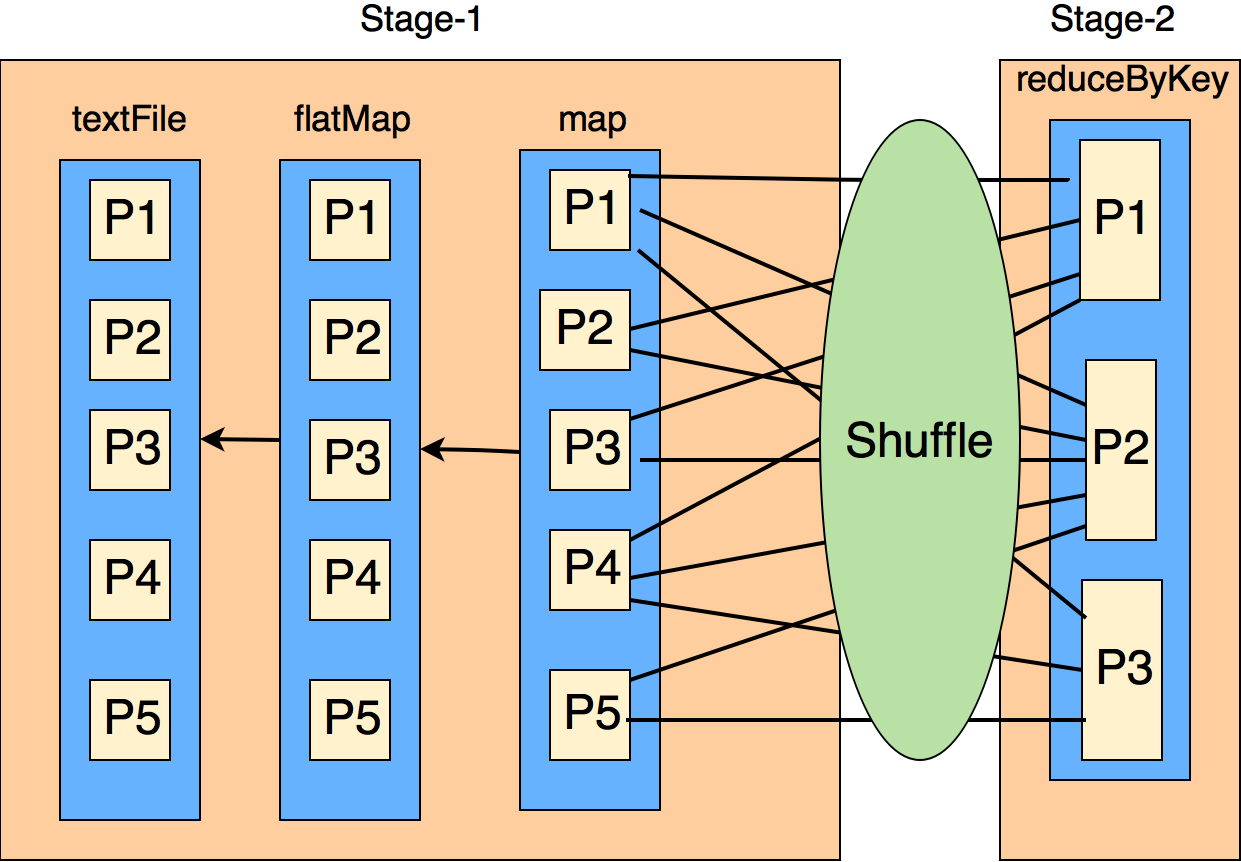
Figure 1-6. Spark’s Shuffle Concept
Since we directed the reduceByKey()
transformation to create 3 partitions,
the result RDD will be partitioned
into 3 chunks as depicted by Figure 4.7.
Shuffle Step for groupByKey()
The groupByKey() shuffle step is
pretty straightforward. It does not
merge the values for the key but
directly the shuffle step happens
and large volume of data gets sent
to each partition (no change is done
to the initial data values). The
merging of values for each key
happens after the shuffle step. For
groupByKey(), a lot of data needs
to be stored on final worker node
(reducer) therefore resulting in
OOM (out of memory error — if
there are lots of data per key).
The shuffle step is demonstrated
below. Note that after groupByKey(),
you do need to call mapValues()
to generate you final desired output.

Figure 1-7. Shuffle Step for groupByKey()
The groupByKey() call makes no
attempt at merging or combining values,
so it’s an expensive operation due to
moving large amount of data over network.
Shuffle Step for reduceByKey()
Per worker node, data is combined so
that at each partition there is at most
one value for each key. Then shuffle
happens and it is sent over the network
to some particular executor for some
action such as reduce. Note that after
reduceByKey(), you do need need to
call mapValues() to generate you
final desired output. In general, a
reduceByKey() can be repalced by a
pair of groupByKey() and mapValues().
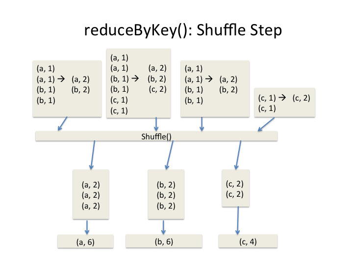
Figure 1-8. Shuffle Step for reduceByKey()
Complete PySpark Solution using reduceByKey()
In its simplest form, reduceByKey() transformation has the following signature (source and target data types — V — must be the same):
reduceByKey(func, numPartitions=None, partitionFunc)
reduceByKey: RDD[(K, V)] --> RDD[(K, V)]
The reduceByKey() transformation, merges
the values for each key using an
*associative* and *commutative* reduce
function. This will also perform the
merging locally on each mapper before
sending results to a reducer, similarly
to a "combiner" in MapReduce. Output
will be partitioned with `numPartitions
partitions, or the default parallelism
level if numPartitions is not specified.
Default partitioner is hash-partition.
Since we want to find the average rating
for all movies rated by a user, and we
know that mean of means is not a mean
function (mean is not a monoid), therefore
we will add up all ratings for a user and
keep track of the number of movies rated:
then (sum_of_ratings, count_of_movies)
is a monoid over an addition function, but
at the end we need one more mapValues()
transformation to find the actual average
rating by dividing sum_of_ratings over
count_of_movies. The complete solution
using reduceByKey() is given below.
Note that reduceBykey() is efficient
and scalable than a groupBykey()
transformation, since merge and combine
are done locally before sending data
for the final reduction.
Step 1: Read Data and Create Pairs
Here we read data and create (key, value)
pairs, where key is a userID and value is
a pair of (rating, 1). To use reduceByKey
for finding average, we need to find the
(sum_of_ratings, number_of_raters). This
is because mean function is not a “monoid”,
so we create (sum_of_ratings, number_of_raters)
to act as a monoid.
-
Read input data and create an
RDD[String]:
>>># spark : SparkSession>>>ratings_path="/tmp/movielens/ratings.csv.no.header">>># rdd: RDD[String]>>>rdd=spark.sparkContext.textFile(ratings_path)>>>rdd.take(3)[u'1,169,2.5,1204927694',u'1,2471,3.0,1204927438',u'1,48516,5.0,1204927435']
-
Transform
RDD[String]toRDD[(String, (Float, Integer))]
>>>defcreate_combined_pair(rating_record):...tokens=rating_record.split(",")...userID=tokens[0]...rating=float(tokens[2])...return(userID,(rating,1))...>>># ratings: RDD[(String, (Float, Integer))]>>>ratings=rdd.map(lambdarec:create_combined_pair(rec))>>>ratings.count()22884377>>>ratings.take(3)[(u'1',(2.5,1)),(u'1',(3.0,1)),(u'1',(5.0,1))]
Create pair RDD
Step 2: Use reduceByKey() to Sum up Ratings
Once (userID, (rating, 1)) pairs are created,
we now can apply the reduceByKey() transformation
to sum up all ratings and raters for a user. The
output of this step will be :
(userID, (sum_of_ratings, number_of_raters)).
>>># x refers to (rating1, frequency1)>>># y refers to (rating2, frequency2)>>># x = (x[0] = rating1, x[1] = frequency1)>>># y = (y[0] = rating2, y[1] = frequency2)>>># x + y = (rating1+rating2, frequency1+frequency2)>>># ratings is the source RDD>>>sum_and_count=ratings.reduceByKey(lambdax,y:(x[0]+y[0],x[1]+y[1]))>>>sum_and_count.count()247753>>>sum_and_count.take(3)[(u'145757',(148.0,50)),(u'244330',(36.0,17)),(u'180162',(1882.0,489))]
Source RDD (
ratings) isRDD[(String, (Float, Integer))]Target RDD (
sum_and_count) isRDD[(String, (Float, Integer))]Notice that the data types for the source and target are the same
Step 3: Find Average Rating
To find average rating per user, we divide “sum of ratings” by the “number of raters”.
>>># x refers to (sum_of_ratings, number_of_raters)>>># x = (x[0] = sum_of_ratings, x[1] = number_of_raters)>>># avg = sum_of_ratings / number_of_raters = x[0] / x[1]>>>avgRating=sum_and_count.mapValues(lambdax:x[0]/x[1])>>>avgRating.take(3)[(u'145757',2.96),(u'244330',2.1176470588235294),(u'180162',3.8486707566462166)]>>>
Complete PySpark Solution using combineByKey()
The combineByKey() is a general and extended
version of reduceByKey() where the result type
can be different than the values being aggregated.
The reduceByKey() ’s limitation is that the
reduced values data types must be the same data
type as input (as defined in the Spark
documentation). This means that, given the
following:
# let rdd represents (key, value) pairs# where value is of type Trdd2=rdd.reduceByKey(lambdax,y:func(x,y))
Then func(x,y) must create a value of type T.
Overall, the combineByKey() transformation
is just such an optimization which aggregates
values for a given key before sending it to
the designated reducer. When using the
combineByKey(), values are aggregated and
merged into one value at each partition then
each partition value is merged into a single
value. Note that the type of the combined
(result) value does not have to match the
type of the original value (which solves the
limitation of reduceByKey()). Using
reduceByKey() or combineByKey(), in
shuffle step, data is combined so each
partition outputs at most one value for each
key to send over the network.
For a given set of (K, V) pairs, combineByKey()
has the following signature (this transformation
has many different versions, here we show the simplest
form):
combineByKey(create_combiner,merge_value,merge_combiners)combineByKey:RDD[(K,V)]-->RDD[(K,C)]VandCcanbedifferentdatatypes.
This is a generic function to combine
the elements for each key using a custom
set of aggregation functions. It converts
an RDD[(K, V)] into a result of type
RDD[(K, C)], for a “combined type” C.
Note that C is a combined data structure.
It can be a simple data type such as Integer
and String or it can be a composite
data structure such as pair (key, value) or
triplet (x, y, z) or any desired data structure.
The C being any data type, makes combineByKey()
a very powerful reducer.
Let the source RDD be RDD[(K, V)]. Then we
have to provide three basic functions:
-
create_combiner:
which turns aV(a single value) into aC(e.g., creates a one-element list of typeC). This is done once per partition.create_combiner: (V) -> C
-
merge_value:
to merge aVinto aC(e.g., adds it to the end of a list). This is applied to every element within a single partition.merge_value: (C, V) -> C
-
merge_combiners:
to combine twoC’s into a single one (e.g., merges the lists). This is applied for two partitions.merge_combiners: (C, C) -> C
To avoid memory allocation, both merge_value
and merge_combiners are allowed to modify
and return their first argument instead of
creating a new C (this can avoid creating
new objects, which can be costly if you have
a lot of data). Finally, note that V and
C can be different data types (in reduceByKey(),
V and C have to be the same data types).
In addition, users can control (by providing
additional parameters) the partitioning of
the output RDD, the serializer that is use
for the shuffle, and whether to perform map-side
aggregation (if a mapper can produce multiple
items with the same key). The combineByKey()
transformation is more general and you have the
flexibility to specify whether you would like
to perform map-side combine. However, it is a
little bit more complex to use (at least you
need to provide 3 small custom functions).
PySpark Solution using combineByKey()
To solve “average rating by user”, we use a pair of (sum_of_ratings, number_of_raters) as a “combined data structure.
Step 1: Read Data and Create Pairs
Here we read data and create (key, value) pairs, where key is a userID and value is rating.
>>># spark : SparkSession>>># create and return a pair of (userID, rating)>>>defcreate_pair(rating_record):...tokens=rating_record.split(",")...return(tokens[0],float(tokens[2]))...>>>key_value_test=create_pair("3,2394,4.0,920586920")>>>key_value_test('3',4.0)>>>ratings_path="/tmp/movielens/ratings.csv.no.header">>>rdd=spark.sparkContext.textFile(ratings_path)>>>rdd.count()22884377>>>ratings=rdd.map(lambdarec:create_pair(rec))>>>ratings.count()22884377>>>ratings.take(3)[(u'1',2.5),(u'1',3.0),(u'1',5.0)]
rdd:RDD[String]ratings:RDD[(String, Float)]
Step 2: Use combineByKey() to Sum up Ratings
Once (userID, rating) pairs are created,
we now can apply the combineByKey()
transformation to sum up all ratings
and number of raters for a user. The
output of this step will be :
(userID, (sum_of_ratings, number_of_raters))
>>># v is a rating from (userID, rating)>>># C represents (sum_of_ratings, number_of_raters)>>># C[0] denotes sum_of_ratings>>># C[1] denotes number_of_raters>>># ratings : source RDD>>>sum_count=ratings.combineByKey((lambdav:(v,1)),(lambdaC,v:(C[0]+v,C[1]+1)),(lambdaC1,C2:(C1[0]+C2[0],C1[1]+C2[1])))>>>sum_count.count()247753>>>sum_count.take(3)[(u'145757',(148.0,50)),(u'244330',(36.0,17)),(u'180162',(1882.0,489))]
RDD[(userID, rating)] = RDD[(String, Float)]RDD[(userID, (sum-of-ratings, count-of-ratings))] = RDD[(String, (Float, Integer))]create_combiner: which turns a
V(a single value) into aCas(V, 1)create_combiner: to merge a
V(rating) into aCas(sum, count)merge_combiners: to combine two
C’s into a singleC
Step 3: Find Average Rating
To find average rating per user, we divide “sum of ratings” by the “number of raters”.
>>># x = (sum_of_ratings, number_of_raters)>>># x[0] = sum_of_ratings>>># x[1] = number_of_raters>>># avg = sum_of_ratings / number_of_raters>>>average_rating=sum_count.mapValues(lambdax:(x[0]/x[1]))>>>average_rating.take(3)[(u'145757',2.96),(u'244330',2.1176470588235294),(u'180162',3.8486707566462166)]
Comparison of Reductions
This chapter presented some of the most important Spark’s reduction transformations (listed below) by simple concrete examples. We discussed the following reducers:
-
reduceByKey() -
groupByKey() -
combineByKey() -
aggregateByKey()
Let’s compare four of the most important
<reducer-name>ByKey() transformations.
Note that, in the following table, V
and C can be different data types.
| Reduction | Source RDD | Target RDD |
|---|---|---|
|
|
|
|
|
|
|
|
|
|
|
|
We learned that some of the reduction transformations
(such as reduceByKey() and combineByKey()) are
preferable over groupByKey() and this is due to the
shuffle step for groupByKey() is more expensive than
the shuffle step for reduceByKey() and combineByKey().
When possible, use reduceByKey() over groupByKey().
Overall, for large volume of data, reduceByKey() and
combineByKey() will scale out better than groupByKey().
This chapter tried to answer few of the key questions such as :
-
Which reduction transformation to use?
-
Which transformation is more efficient?
-
When to use
reduceByKey()overgroupByKey()?
To understand reduction transformation we need to understand the following:
-
The underlying architecture of the reduction transformations
-
The “shuffle phase” of the reduction transformations (the most important)
We learned that in Shuffle Step of
reduceByKey(): the data is combined
(and less data is sent over network) so
that at each partition there is at most
one value for each key and then shuffle
happens and it is sent over the network
to some particular executor for some
action such as reduce. While in
groupByKey() Shuffle Step: it does
not merge the values for the key but
directly the shuffle step happens and
lots of data gets sent to each partition,
almost same as the initial data. In
groupByKey() the merging of values
for each key happens after the shuffle
step and lots of data needs to be stored
on final worker node (reducer) thereby
resulting (may be) in out of memory problem.
While both of these Spark transformations
(reduceByKey() and groupByKey()) will
produce the correct answer, the
reduceByKey() works much better on a
large dataset. That’s because Spark knows
it can combine output with a common key
on each partition before shuffling the
data. You may use combineByKey() when
you are combining elements but your return
type differs from your input value type.
When possible, you should replace
groupByKey() with reduceByKey() to
improve scalability and performance (in
some cases). The reduceByKey()
transformation performs map side combine
which can reduce network IO and shuffle
size where as groupByKey() will not
perform any map side combine at all.
We found out that the aggregateByKey()
transformation is more suitable for compute
aggregations for keys, example aggregations
such as sum, average, variance, etc. The
important rule here is that the extra
computation spent for map side combine can
reduce the size sent out to other worker
nodes and driver. If your requirements
satisfies this rule, you probably should
use aggregateByKey() (at minimum, you
need to implement three basic functions:
create_combiner, merge_value, and
merge_combiners — these functions
were discussed in the early sections of
this chapter.
Summary
-
The
reduceByKey()transformation is more efficient when we run this on large data set. This transformation’s output type has to be the same as input value types. -
The
combineByKey()transformation is a generic reduction and does not have restrictions of thereduceByKey(): output type can be different form input types. -
When possible, avoid
groupByKey()on big data, which can cause “out of memory” and “out of disk space” Problems. -
When possible, use
reduceByKey()orcombineByKey()overgroupByKey() -
Make sure that your reducer is a monoid, otherwise you might get wrong reduced values.