
“Archimedes’ finding that the crown was of gold was a discovery; but he invented the method of determining the density of solids. Indeed, discoverers must generally be inventors; though inventors are not necessarily discoverers.”
—William Ramsay, 1852–1916, Chemist
The forces that exist within a fluid at any point may arise from various sources. These include gravity, or the “weight” of the fluid, an imposed static pressure from an external source, an external driving force such as a pump or compressor, and the internal resistance to relative motion between fluid elements, or inertial effects resulting from the local velocity and the mass flow rate of the fluid (e.g., the transport or rate of change of momentum).
Any or all of these forces may result in local stresses within the fluid. “Stress” can be thought of as a (local) “concentration of force,” or the local force per unit area that acts upon an infinitesimal volume of the fluid. Now both force and area are vectors, the direction of the area being defined by the normal vector that points outward relative to the fluid volume bounded by the surface. Thus, each stress component has a magnitude and two directions associated with it, that is, the direction of the force that acts on the fluid element, Fj, and the orientation of the surface of the element upon which the force acts, Ai. These are the characteristics of a “second-order tensor” or “dyad.” If the direction in which the local force acts is designated by subscript j (e.g., j = x, y, or z in Cartesian coordinates) and the orientation (i.e., the normal to the surface) of the local area element upon which it acts is designated by the subscript i, then the corresponding stress component (σij,) is given by
(4.1) |
Note that since i and j each represent any of three possible directions, there are a total of nine possible components of the stress tensor (at any given point in a fluid). However, it can readily be shown that the stress tensor is symmetric (i.e., the ij components are the same as the ji components for i≠j) so there are at most six independent stress components. Of these six, three are normal components (i = j) and three are tangential (i ≠ j) components of the stress tensor. Because of the various origins of these forces, as mentioned earlier, there are different “types” of stresses. For example, the only stress that can exist in a fluid at rest is pressure, which can result from gravity (e.g., hydrostatic head) or various other static forces acting on the fluid. Although pressure is a stress (e.g., a force per unit area), it is isotropic, that is, the pressure at a point acts uniformly in all directions, normal to any local surface at a given point in the fluid. Such a stress has no directional character and is thus a scalar. (Any isotropic tensor is, by definition, a scalar, because it has magnitude only and no direction.) However, the stress components that arise from the fluid motion do have directional characteristics, which are determined by the relative motion (or rather by the local velocity gradients) present in the fluid. These stresses are associated with the local resistance to motion due to viscous or inertial properties and are anisotropic in nature, that is, their components depend upon direction at any given point in the fluid. These anisotropic stress components are designated by τij, where the i and j have the same significance as in Equation 4.1.
Thus, the total stress, σij, at any point within a fluid is composed of both the isotropic pressure and anisotropic stress components, as follows:
(4.2) |
where P is the (isotropic) pressure. By convention, tensile stresses are considered positive and compressive stresses are negative, so that pressure is a “negative” stress because it is always compressive, whereas tensile stresses are positive (i.e., a positive Fj acting on a positive Ai or a negative Fj on a negative Ai). The term δij in Equation 4.2 is a “unit tensor” (or Kronecker delta), which has a value of zero if i ≠ j, and unity if i = j. This is required, because the isotropic pressure acts only in the normal direction (e.g., i = j) and has only one component (i.e., it is a scalar). As mentioned earlier, the anisotropic shear stress components τij in a fluid are associated with relative motion within the fluid and are therefore zero in any fluid at rest. It follows that the only stress that can exist in a fluid at rest or in a state of uniform motion (in which there are no velocity gradients present in the fluid) is pressure. This is a major distinction between a fluid and a solid, since solids can support a shear stress in a state of rest. It is this situation with which we will be concerned in this chapter.
In Cartesian coordinates, the components of the stress tensor are
(4.3) |
Example 4.1 Flow in a Vertical Slit
Consider a Newtonian liquid contained in a slit between two vertical parallel planes (see Figure E4.1). For case (a), the slit is closed at the bottom so that the fluid cannot flow out. For case (b), the slit is open at the bottom so that the liquid can flow out. If the coordinate system is as shown in the diagram, show the nonzero components of the stress tensor for both case (a) and (b).
Solution:
Case (a): As there is no motion, then all shear stresses are zero, so

Figure E4.1 Flow in a vertical slit.
Case (b): As there is motion only in the −z direction and the z component of velocity varies only in the x direction (i.e., the fluid sticks to the walls, so the velocity must be zero at the walls and nonzero away from the walls), then the shear stress components must be τxz = τzx:
Note that τxz = τzx due to symmetry of the stress tensor.
“Students often feel under stress and pressure when trying to understand pressure and stress.”
II. THE BASIC EQUATION OF FLUID STATICS
Consider a cylindrical region of arbitrary size and shape within a fluid, as shown in Figure 4.1. We will apply a momentum balance to a “slice” of the fluid that has a z area Az, a thickness Δz and is located a vertical distance z above some horizontal reference plane. The density of the fluid in the slice is ρ, and the force of gravity (g) acts in the −z direction. A momentum balance on a “closed” system (e.g., the slice) is equivalent to Newton’s second law of motion, that is,
(4.4) |
Because this is a vector equation, we apply it to the z vector components. is the sum of all of the forces acting on the system (the “slice”) in the z direction, m is the mass of the system, and az is the acceleration in the z direction. Since the fluid is not moving, az = 0, and the momentum balance reduces to a force balance. The z forces acting on the system include the (−) pressure on the bottom (at z), times the (−) z area, the (−) pressure on the top (at z +Δz), times the (+) z area, and the z component of gravity, that is, the “weight” of the fluid, (−ρgAzΔz). The first force is positive, and the latter two are negative because they act in the (−z) direction. The momentum (force) balance thus becomes
(4.5) |

FIGURE 4.1 Arbitrary region within a fluid.
If we divide through by AzΔz, then take the limit as the thickness of the slice shrinks to zero (Δz → 0), the result is
(4.6) |
which is the basic equation of fluid statics. This equation states that at any point within a given fluid the pressure decreases as the elevation (z) increases, at a local rate that is equal to the product of the fluid density and the gravitational acceleration at that point. This equation is valid at all points within any given static fluid regardless of the nature of the fluid (irrespective of whether the fluid is Newtonian or non-Newtonian, compressible or incompressible). We shall now show how the equation can be applied to various special situations.
If the density (ρ) is constant, the fluid is referred to as “isochoric” (i.e., a given mass occupies a constant volume), although the somewhat more restrictive term “incompressible” is commonly used for this property (liquids are considered to be incompressible or isochoric fluids under most conditions). If gravity (g) is also constant, the only variables in Equation 4.6 are pressure and elevation. This can then be integrated between any two points (1 and 2) in a given fluid to give
(4.7) |
which can also be written as
(4.8) |
where
(4.9) |
This says that the sum of the local pressure (P) and static head (ρgz), that is, the potential (Φ), is constant at all points within a given isochoric (incompressible) non-flowing fluid. This is an important result for such fluids, and it can be applied directly to determine how the pressure varies with elevation in a static liquid, as illustrated by the following example.
Example 4.2 Manometer Attached to Pressure Taps on a Pipe Carrying a Flowing Fluid
The pressure difference between two points in a fluid (flowing or static) can be measured using a manometer. The manometer contains a static incompressible liquid (density ρm) that is immiscible with the fluid flowing in the pipe (density ρf). The legs of the manometer are connected to taps on the pipe where the pressure difference is desired (see Figure E4.2). By applying Equation 4.8 to any two points within either one of the fluids within the manometer, we see that
(4.10) |
or
(4.11) |

Figure E4.2 Manometer.
When these three equations are added, P3 and P4 cancel out. The remaining terms can be collected to give
(4.12) |
where Φ = P+ ρgz and ΔΦ = Φ2 – Φ1, Δρ = ρm – ρf, Δh = z4 − z3. Equation 4.12 is the basic manometer equation and can be applied to a manometer in any orientation. Note that the manometer reading (Δh) is a direct measure of the potential difference (Φ2 − Φ1), which is identical to the pressure difference (P2 − P1) only if the pipe is horizontal (i.e., z2 = z1). It should be noted that these static fluid equations, Equations 4.10 through 4.12, apply only within the manometer but not within the pipe, as the fluid in the pipe is not static.
Example 4.3 Barometer
A straightforward and most common application of Equation 4.8 is seen in the everyday mercury barometer used to measure the atmospheric pressure. In its basic form, a glass tube filled with mercury is inverted so that its open end is well submerged in a mercury reservoir as shown in Figure E4.3. Determine the relation between the height of the mercury in the barometer (z1) and the local atmospheric pressure.

Figure E4.3 Barometer.
Solution:
Applying Equation 4.8 to points 1 and 2
or
Since the mercury at point 2 is at the same level in a common (static) fluid both inside and outside the barometer and is in contact with the open atmosphere, P2 = 1 atm = 101,325 Pa. Similarly, the space above the level of mercury at point 1 is filled with mercury vapor. Therefore, pressure at point 1 is equal to the vapor pressure of mercury, which is negligibly small, for example, at 300 K, the vapor pressure of mercury is about 0.3 Pa and hence P1 ~ 0. The density of mercury at 20°C is 13,500 kg/m3, so that substituting these values into the above equation gives
This yields which is the value reported in most weather reports in newspapers and TV.
If the fluid can be described by the ideal gas law (e.g., air under normal atmospheric conditions follows this law quite well), then
(4.13) |
and Equation 4.6 becomes
(4.14) |
Now if gravity and temperature are constant for all values of z of interest (i.e., isothermal conditions), Equation 4.14 can be integrated from (P1, z1) to (P2, z2) to give the pressure as a function of elevation:
(4.15) |
where Δz = z2 − z1. Notice that in this case the pressure drops exponentially as the elevation increases, instead of linearly as for the incompressible fluid.
If there is no heat transfer or energy dissipated in the gas when going from state 1 to state 2, the process is adiabatic and reversible, that is, isentropic. For an ideal gas under these conditions,
(4.16) |
where k = cp/cv is the specific heat ratio for the gas (for an ideal gas, cp = cv+R/M). If the density is eliminated from Equations 4.16 and 4.13, the result is
(4.17) |
which relates the temperature and pressure at any two points in an isentropic ideal gas. If Equation 4.17 is used to eliminate T from Equation 4.14, the latter can be integrated to give the pressure as a function of elevation:
(4.18) |
which is a nonlinear relationship between pressure and elevation. Equation 4.15 can be used to eliminate P2/P1 from this equation to give an expression for the temperature as a function of elevation under isentropic conditions:
(4.19) |
This indicates that the temperature drops linearly as the elevation increases.
Neither Equation 4.15 nor Equation 4.18 would be expected to provide a very good representation of the pressure and temperature in the real atmosphere, which is neither isothermal nor isentropic. Thus, we must resort to the use of observations (i.e., empiricism) to describe the real atmosphere. In fact, atmospheric conditions vary considerably from time to time and from place to place over the earth. However, a reasonable representation of atmospheric conditions “averaged” over the year and over the earth based on observations results in the following:
(4.20) |
where the average temperature at ground level (z = 0) is assumed to be 15°C (288 K). These equations describe what is known as the “standard atmosphere” which represents an average state over the world and throughout the year. Using Equation 4.20 for the temperature as a function of elevation and incorporating this into Equation 4.14 gives
(4.21) |
where
To = 288 K
G = 6.5° C/km
Integrating Equation 4.21, assuming that g is constant, gives the pressure as a function of elevation:
(4.22) |
This applies for 0 < z < 11 km.
We have stated that the only stress that can exist in a fluid at rest is pressure, because the shear stresses (which resist motion) are zero when the fluid is at rest. This also applies to fluids in motion provided there is no relative motion within the fluid (the shear stresses are determined by the velocity gradients, e.g., the shear rate). However, if the motion involves a uniform acceleration, this can contribute an additional component to the pressure, as illustrated by the examples in this section.
Consider the vertical column of fluid illustrated in Figure 4.1, but now imagine it to be on an elevator that is accelerating upward with an acceleration of az, as illustrated in Figure 4.2. Application of the momentum balance to the “slice” of fluid, as before, gives
(4.23) |
which is the same as Equation 4.3, except that now az ≠ 0. The same procedure that led to Equation 4.6 now gives
(4.24) |
which shows that the effect of a superimposed upward vertical acceleration is equivalent to increasing the gravitational acceleration by an amount az (which is why you feel “heavier” on a rapidly accelerating elevator). In fact, this result may be generalized to any direction, that is, an acceleration in the i direction will result in a pressure gradient within the fluid in the −i direction of magnitude ρai:
(4.25) |
Two applications of this equation are illustrated in the following sections.
B. HORIZONTALLY ACCELERATING FREE SURFACE
Consider a pool of water in the bed of your pickup truck. If you accelerate from rest, the water will slosh toward the rear, and you want to know how fast you can accelerate (ax) without spilling the water out of the back of the truck (see Figure 4.3). That is, you must determine the slope (tan θ) of the water surface as a function of the rate of acceleration (ax). Now at any point within the liquid there is a vertical pressure gradient due to gravity (Equation 4.6) and a horizontal pressure gradient due to the acceleration ax (Equation 4.25). Thus, at any location within the liquid, the total differential pressure dP between two points separated by a small distance dx in the horizontal direction and dz in the vertical direction is given by

FIGURE 4.2 Vertically accelerating column of fluid.
(4.26) |

FIGURE 4.3 Horizontally accelerating tank.
Because the surface of the water is open to the atmosphere where P = constant (1 atm), one can apply Equation 4.26 on the free surface as
(4.27) |
or
(4.28) |
which is the slope of the surface and is seen to be independent of fluid properties. Knowledge of the initial position of the surface plus the surface slope determines the elevation of the water level at the rear of the truck bed and hence whether or not the water will spill out.
Consider an open bucket of water resting on a turntable that is rotating at an angular velocity ω (see Figure 4.4). The (inward) radial acceleration due to the rotation is ω2r, which results in a corresponding radial pressure gradient at all points in the fluid, in addition to the vertical pressure gradient due to gravity. Thus, the pressure differential between any two points within the fluid separated by dr and dz is
(4.29) |
Just as for the accelerating tank, the shape of the free surface can be determined from the fact that the pressure is constant at the free surface, that is,
(4.30) |

FIGURE 4.4 Rotating fluid.
This can be integrated to give an equation for the shape of the surface:
(4.31) |
which shows that the shape of the rotating surface is parabolic.
As a consequence of Archimedes’ principle, the buoyant force exerted on a submerged body is equal to the weight of the displaced fluid, and it acts in a direction opposite to the gravity vector. Thus, the “effective net weight” of a submerged body is its actual weight (in air) less the weight of an equal volume of the fluid. The result is equivalent to replacing the density of the body (ρs) in the expression for its weight (, where is the volume of the solid body) by the difference between the density of the body and that of the fluid (i.e., , where Δρ = ρs − ρf).
This also applies to a body submerged in a fluid that is subject to any acceleration. For example, a solid particle of volume submerged in a fluid within a centrifuge at a point r where the angular velocity is ω is subjected to a net radial force equal to . Thus, the effect of buoyancy is to effectively reduce the density of the body by an amount equal to the density of the surrounding fluid.
V. STATIC FORCES ON SOLID BOUNDARIES
The force exerted on a solid boundary by a static pressure is given by
(4.32) |
Note that both force and area are vectors, whereas pressure is a scalar. Hence, the directional character of the force is determined by the orientation of the surface on which the pressure acts. That is, the component of force acting in a given direction on a surface is the integral of the pressure over the projected component area of the surface normal to the direction of the force vector. The surface vector that is normal to the surface is parallel to the direction of the force (recall that pressure is a negative isotropic stress and the outward normal to the [fluid] system boundary represents a positive area). Also, from Newton’s third law (“action equals reaction”), the force exerted on the fluid system boundary is of opposite sign to the force exerted by the fluid system on the solid boundary.
Example 4.4
Consider the force within the wall of a pipe resulting from the pressure of the fluid inside the pipe, as illustrated in Figure E4.4.
The pressure P acts equally in all directions on the inside wall of the pipe. The resulting force exerted within the pipe wall normal to a vertical (or any other orientation) plane through the pipe axis is simply the product of the pressure and the projected area of the inside pipe wall on this plane, for example, Fx = PAx = 2PRL. This force acts to pull the metal in the wall apart and is resisted by the internal stress within the metal holding it together. This is the effective working stress, σ, of the particular material of which the pipe is made, acting on the cross section of pipe wall, or 2σtL. If we assume a thin-walled pipe (i.e., we neglect the radial variation of the stress from point to point within the wall), a force balance between the “disruptive” pressure force and the “restorative” force due to the internal stress in the metal gives
(4.33) |
or
(4.34) |
This relation determines the pipe wall thickness (t) required to withstand a fluid pressure P in a pipe of radius R made of a material with a working stress σ. The dimensionless pipe wall thickness (times 1000) is known as the Schedule number of the pipe:
(4.35) |
This expression is only approximate, as it does not make any allowance for the effects of such things as pipe threads, corrosion, or wall damage. To compensate for these factors, an additional allowance is made for the wall thickness in the working definition of the “schedule thickness,” ts:
(4.36) |

Figure E4.4 Fluid pressure inside a pipe.
where both ts and Do (the pipe outside diameter) are measured in inches, and the factor of 200 allows for damage, threads, etc., on the pipe wall. This relation between schedule number and pipe dimensions can be compared with the actual dimensions of commercial pipes for various schedule pipe sizes, as tabulated in Appendix F.
Example 4.5
A composite block made up of concrete and iron weighs 500 N in air and only 280 N in fresh water (density 1000 kg/m3). Calculate the specific gravity of the block.
Solution:
For the given data, one can draw the free body diagram with various forces acting on the block as shown in Figure E4.5. A force balance in the vertical direction yields
or
By definition, the buoyancy force is given by
Specific gravity of the block is 2.27.
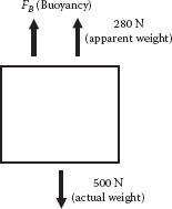
Figure E4.5 Submerged block.
Example 4.6
Calculate the pressure at the bottom of the tank shown in Figure E4.6. Also, calculate the magnitude and direction of the force (per unit width) exerted on the door at the bottom, with dimensions A (height) and B (width).
Solution:
The pressure is calculated at the bottom of the tank by successive application of Equation 4.8 across points 1, 2, 3, that is,
In terms of pressure and density,
Now using ϕ1 =ϕ3′
which is the pressure at the bottom of the tank.
In order to calculate the force on the door due to the pressure, Equation 4.32 can be applied to a differential area B dz, where B is the width of the door, oriented in the −x direction. This force has only one component, in the x direction:

Figure E4.6 Tank Containing oil and water.
The pressure at any height z acting on the door is
or
This force acts in the positive x direction on the door with dimensions AB per unit width (B).
The key points covered in this chapter include
• Pressure/stress in static and uniformly moving systems
• The basic equation of fluid statics
• The manometer equation
• Pressure distribution in static gases
• Pressure distribution in uniformly rotating and accelerating systems
• Static forces on solid boundaries—pipe wall stress
STATICS
1. The manometer equation is ΔΦ = −ΔρgΔh, where ΔΦ is the difference in the total pressure plus static head (P+ ρgz) between the two points to which the manometer is connected, Δρ is the difference in the densities of the two fluids in the manometer, Δh is the manometer reading, and g is the acceleration due to gravity. If Δρ is 12.6 g/cm3 and Δh is 6 in. for a manometer connected to two points on a horizontal pipe, calculate the value of ΔP in the following units:
(a) dyn/cm2; (b) pascals; (c) atm.
2. A manometer containing an oil with specific gravity (SG) = 0.92 is connected across an orifice plate in a horizontal pipeline carrying seawater (SG = 1.1). If the manometer reading is 16.8 cm, what is the pressure drop across the orifice in psi? What is it in inches of water?
3. A mercury manometer is used to measure the pressure drop across an orifice that is mounted in a vertical pipe. A liquid with a density of 0.87 g/cm3 is flowing upward through the pipe and the orifice. The distance between the manometer taps is 1 ft. If the pressure in the pipe at the upper tap is 30 psig and the manometer reading is 15 cm, what is the pressure in the pipe at the lower manometer tap in psig?
4. A mercury manometer is connected between two points in a piping system that contains water. The downstream tap is 6 ft higher than the upstream tap, and the manometer reading is 16 in. If a pressure gage in the pipe at the upstream tap reads 40 psia, what would a pressure gage at the downstream tap read in (a) psia, (b) dyn/cm2, (c) Pa, (d) kgf/m2?

Figure P4.5 Inclined manometer (not to scale).
5. An inclined tube manometer with a reservoir is used to measure the pressure gradient in a large pipe carrying oil (SG = 0.91) (see Figure P4.5). The pipe is inclined at an angle of 60° to the horizontal, and flow is uphill. The manometer tube is inclined at an angle of 20° to the horizontal, and the pressure taps on the pipe are 5 in. apart. The manometer reservoir diameter is eight times as large as the manometer tube diameter, and the manometer fluid is water. If the manometer reading (l) is 3 in. and the displacement of the interface in the reservoir is neglected, what is the pressure drop in the pipe in (a) psi, (b) Pa, (c) in. H2O? What is the percentage error introduced by neglecting the change in elevation of the interface in the reservoir?
6. Water is flowing downhill in a pipe that is inclined 30° to the horizontal. A mercury manometer is attached to pressure taps 5 cm apart on the pipe. The interface in the downstream manometer leg is 2 cm higher than the interface in the upstream leg. What is the pressure gradient (ΔP/L) in the pipe in (a) Pa/m, (b) dyn/cm3, (c) in. H2O/ft, (d) psi/mi?
7. Repeat Problem 6 for the case in which the water in the pipe is flowing uphill instead of downhill, all other conditions remaining the same.
8. Two horizontal pipelines are parallel, with one carrying salt water (ρ = 1.988 slugs/ft3) and the other carrying fresh water (ρ = 1.937 slugs/ft3). An inverted manometer using linseed oil (ρ = 1.828 slugs/ft3) as the manometer fluid is connected between the two pipelines. The interface between the oil and the fresh water in the manometer is 38 in. above the centerline of the freshwater pipeline, and the oil/salt water interface in the manometer is 20 in. above the centerline of the salt water pipeline. If the manometer reading is 8 in., determine the difference in the pressures between the pipelines in (a) Pa and in (b) psi.
9. Two identical tanks are 3 ft in diameter and 3 ft high, and they are both vented to the atmosphere. The top of tank B is level with the bottom of tank A, and they are connected by a line from the bottom of A to the top of B with a valve in it. Initially A is full of water, and B is empty. The valve is opened for a short time, letting some of the water drain into B. An inverted manometer having an oil with SG = 0.7 is connected between taps on the bottom of each tank. The manometer reading is 6 in., and the oil/water interface in the leg connected to tank A is higher. What is the water level in each of the tanks?

FIGURE P4.10 Manometer on pipe bend.
10. An inclined tube manometer is used to measure the pressure drop in an elbow through which water is flowing (see Figure P4.10). The manometer fluid is an oil with SG = 1.15. The distance L is the distance along the inclined tube that the interface has moved from its equilibrium (no pressure differential) position. If h = 6 in., L = 3 in., θ = 30°, the reservoir diameter is 2 in., and the tubing diameter is 0.25 in., calculate the pressure drop (P1 − P2) in (a) atm; (b) Pa; (c) cmH2O, and; (d) dyn/cm2. What would be the percentage error in pressure difference as read by the manometer if the change in level in the reservoir is neglected?
11. The three-fluid manometer illustrated in Figure P4.11 is used to measure a very small pressure difference (P1 − P2). The cross-sectional area of each of the reservoirs is A and that of the manometer legs is a. The three fluids have densities ρa, ρb, and ρc, and the difference in elevation of the interfaces in the reservoir is x. Derive the equation that relates the manometer reading h to the pressure difference (P1 − P2). How would the relation be simplified if A≫a?

FIGURE P4.11 Three fluid manometer.

FIGURE P4.13 Manometer on inclined tube.
12. A tank that is vented to the atmosphere contains a liquid with a density of 0.9 g/cm3. A dip tube inserted into the top of the tank extends to a point 1 ft from the bottom of the tank. Air is bubbled slowly through the dip tube, and the air pressure in the tube is measured with a mercury (SG = 13.6) manometer. One leg of the manometer is connected to the air line feeding the dip tube, and the other leg is open to the atmosphere. If the manometer reading is 5 in., what is the depth of the liquid in the tank?
13. An inclined manometer is used to measure the pressure drop between two taps on a pipe carrying water, as shown in Figure P4.13. The manometer fluid is an oil with SG = 0.92, and the manometer reading (L) is 8 in. The manometer reservoir is 4 in. in diameter, the tubing is 1/4 in. in diameter, and the manometer tube is inclined at an angle of 30° to the horizontal. The pipe is inclined at 20° to the horizontal, and the pressure taps are 40 in. apart.
(a) What is the pressure difference between the two pipe taps that would be indicated by the difference in readings of two pressure gages attached to the taps, in (1) psi, (2) Pa, and (3) in. H2O?
(b) Which way is the water flowing?
(c) What would the manometer reading be if the valve were closed?
14. The pressure gradient required to force water through a straight horizontal 1/4 in. ID tube at a rate of 2 gpm is 1.2 psi/ft. Consider this same tubing coiled in an expanding helix with a vertical axis. Water enters the bottom of the coil and flows upward at a rate of 2 gpm. A mercury manometer is connected between two pressure taps on the coil, one near the bottom where the coil radius is 6 in., and the other near the top where the coil radius is 12 in. The taps are 2 ft apart in the vertical direction, and there is a total of 5 ft of tubing between the two taps. Determine the manometer reading, in cm.
15. It is possible to achieve a weightless condition for a limited time in an airplane by flying in a circular arc above the earth (like a rainbow). If the plane flies at 650 mph, what should the radius of the flight path be (in miles) to achieve weightlessness?
16. Water is flowing in a horizontal pipe bend at a velocity of 10 ft/s. The radius of curvature of the inside of the bend is 4 in., and the pipe ID is 2 in. A mercury manometer is connected to taps located radially opposite to each other on the inside and outside of the bend. Assuming that the water velocity is uniform over the pipe cross section, what would be the manometer reading in centimeters? What would it be if the water velocity were 5 ft/s? Convert the manometer reading to equivalent pressure difference in psi and Pa.
17. Calculate the atmospheric pressure at an elevation of 3000 m, assuming (a) air is incompressible, at a temperature of 59°F; (b) air is isothermal at 59°F and an ideal gas; (c) the pressure distribution follows the model of the standard atmosphere, with a temperature of 59°F at the surface of the earth.
18. One pound mass of air (MW = 29) at sea level and 70°F is contained in a balloon, which is then carried to an elevation of 10,000 ft in the atmosphere. If the balloon offers no resistance to expansion of the gas, what is its volume at this elevation?
19. A gas well contains hydrocarbon gases with an average molecular weight of 24, which can be assumed to be an ideal gas with a specific heat ratio of 1.3. The pressure and temperature at the top of the well are 250 psig and 70°F, respectively. The gas is being produced at a slow rate, so that the conditions in the well can be considered to be isentropic.
(a) What are the pressure and temperature at a depth of 10,000 ft?
(b) What would the pressure be at this depth if the gas were assumed to be isothermal?
(c) What would the pressure be at this depth if the gas were assumed to be incompressible?
20. The adiabatic atmosphere obeys the equation
where
k is a constant
ρ is density
If the temperature decreases 0.3°C for every 100 ft increase in altitude, what is the value of k? [Note: Air is an ideal gas; g = 32.2 ft/s2; R = 1544 ft lbf/(°R lbmol).
21. Using the actual dimensions of commercial steel pipe from Appendix F, plot the pipe wall thickness versus the pipe diameter for both Schedule 40 and Schedule 80 pipes, and fit the plot with a straight line by linear regression analysis. Rearrange your equation for the line in a form consistent with the given equation for the schedule number as a function of the wall thickness and diameter:
and use the results of the regression to calculate values corresponding to the parameters 1750 and 200 in this equation. Do this using (for D) (a) the nominal pipe diameter and (b) the outside pipe diameter. Explain any discrepancies or differences in the numerical values determined from the data fit compared to those in the equation.
22. The “yield stress” for carbon steel is 35,000 psi, and the “working stress” is one-half of this value. What schedule number would you recommend for a pipe carrying ethylene at a pressure of 2500 psi if the pipeline design calls for a pipe of 2 in. ID? Give the dimensions of the pipe that you would recommend. What would be a safe maximum pressure to recommend for this pipe?
23. Consider a 90° elbow in a 2 in. pipe (all of which is in the horizontal plane). A pipe tap is drilled through the wall of the elbow on the inside curve of the elbow, and another through the outer wall of the elbow directly across from the inside tap. The radius of curvature of the inside of the bend is 2 in., and that of the outside of the bend is 4 in. The pipe is carrying water, and a manometer containing an immiscible oil with SG of 0.90 is connected across the two taps on the elbow. If the reading of the manometer is 7 in., what is the average velocity of the water in the pipe, assuming that the flow is uniform across the pipe inside the elbow?
24. A pipe carrying water is inclined at an angle of 45° to the horizontal. A manometer containing a fluid with SG of 1.2 is attached to taps on the pipe, which are 1 ft apart. If the liquid interface in the manometer leg that is attached to the lower tap is 3 in. below the interface in the other leg, what is the pressure gradient in the pipe (ΔP/L), in units of (a) psi/ft and (b) Pa/m? Which direction is the water flowing?
25. A tank contains a liquid of unknown density (see Figure P4.25). Two dip tubes are inserted into the tank, each to a different level in the tank, through which air is bubbled very slowly through the liquid. A manometer is used to measure the difference in pressure between the two dip tubes. If the difference in level of the ends of the dip tubes (H) is 1 ft, and the manometer reads 1.5 ft (h) with water as the manometer fluid, what is the density of the liquid in the tank?
26. The tank shown in Figure P4.26 has a partition that separates two immiscible liquids. Most of the tank contains water, and oil is floating above the water on the right of the partition. The height of the water in the standpipe (h) is 10 cm, and the interface between the oil and water is 20 cm below the top of the tank and 25 cm above the bottom of the tank. If the specific gravity of the oil is 0.82, what is the height of the oil in the standpipe (H)?
27. A manometer that is open to the atmosphere contains water, with a layer of oil floating on the water in one leg (see Figure P4.27). If the level of the water in the left leg is 1 cm above the center of the leg, the interface between the water and oil is 1 cm below the center in the right leg, and the oil layer on the right extends 2 cm above the center, what is the density of the oil?

FIGURE P4.25 Manometer measuring density of liquid.

FIGURE P4.26 Immiscible fluids in tank.

FIGURE P4.27 Density of oil in two-fluid manometer.
28. An open cylindrical drum, with a diameter of 2 ft and a length of 4 ft, is turned upside down in the atmosphere and then submerged in a liquid so that it floats partially submerged upside down, with air trapped inside. If the drum weighs 150 lbf, and it floats with 1 ft extending above the surface of the liquid, what is the density of the liquid? How much additional weight must be added to the drum to make it sink to the point where it floats just level with the liquid?
29. A solid spherical particle with a radius of 1 mm and a density of 1.3 g/cm3 is immersed in water in a centrifuge. If the particle is 10 cm from the axis of the centrifuge, which is rotating at a rate of 100 rpm, what direction will the particle be traveling relative to a horizontal plane?
30. A manometer with mercury as the manometer fluid is attached to the wall of a closed tank containing water (see Figure P4.30). The entire system is rotating about the axis of the tank at N rpm. The radius of the tank is r1, the distances from the tank centerline to the manometer legs are r2 and r3 (as shown), and the manometer reading is h. If N = 30 rpm, r1 = 12 cm, r2 = 15 cm, r3 = 18 cm, and h = 2 cm, determine the gage pressure at the wall of the tank and also at the centerline at the level of the pressure tap on the tank.

FIGURE P4.30 Revolving manometer.
31. With reference to Figure P4.30, the manometer contains water as the manometer fluid and is attached to a tank that is empty and open to the atmosphere. When the tank is stationary, the water level is the same in both legs of the manometer. If the entire system is rotated about the centerline of the tank at a rate of N (rpm):
(a) What happens to the water levels in the legs of the manometer?
(b) Derive an equation for the difference in elevation of the levels (h) in the legs of the manometer as a function of known quantities.
32. You want to measure the specific gravity of a liquid. To do this, you first weigh a beaker of the liquid on a scale (WLo). You then attach a string to a solid body that is heavier than the liquid and while holding the string you immerse the solid body in the liquid and measure the weight of the beaker containing the liquid with the solid submerged (WLs). You then repeat the same procedure using the same weight but with water instead of the “unknown” liquid. The corresponding weight of the water without the weight submerged is WWo and with the solid submerged is WWs. Show how the specific gravity of the “unknown” liquid can be determined from these four weights, and show that the result is independent of the size, shape, or weight of the solid body used (provided, of course, that it is heavier than the liquids and is large enough that the difference in the weights can be measured precisely).
33. A vertical U-tube manometer is open to the atmosphere and contains a liquid that has a SG of 0. 87 and a vapor pressure of 450 mmHg at the operating temperature. The vertical tubes are 4 in. apart, and the level of the liquid in the tubes is 6 in. above the bottom of the manometer. The manometer is then rotated about a vertical axis through its centerline. Determine what the rotation rate would have to be (in rpm) for the liquid to start to boil.
34. A spherical particle with SG = 2.5 and a diameter of 2 mm is immersed in water in a cylindrical centrifuge with a diameter of 20 cm. If the particle is initially 8 cm above the bottom of the centrifuge and 1 cm from the centerline, what is the speed of the centrifuge (in rpm) if this particle strikes the wall of the centrifuge just before it hits the bottom?
A |
Area, [L2] |
Ai |
Bounding area component with outward normal in the i direction, [L2] |
az |
Acceleration in the z direction, [L/t2] |
cp |
Specific heat at constant pressure {FL/MT = [L2/Mt2] |
cv |
Specific heat at constant volume {FL/MT = [L2/Mt2] |
Do |
Pipe diameter (outer), [L] |
Fj |
Force in the j direction, [F = ML/t2] |
G |
Atmospheric temperature gradient (= 6.5°C/km), [T/L] |
g |
Acceleration due to gravity, [L/t2] |
h |
Vertical displacement of manometer interface, [L] |
k |
Isentropic exponent (= cp/cv for ideal gas), [—] |
M |
Molecular weight, [M/mol] |
P |
Pressure, [F/L2 = M/Lt2] |
R |
Gas constant, [FL/(mol T) = M L2 (mole t2 T)] |
r |
Radial direction, [L] |
T |
Temperature, [T] |
t |
Pipe thickness, [L] |
Volume, [L3] |
|
z |
Vertical direction, measured upward, [L] |
GREEK
Δ() |
Difference between two values, [= ()2 – ()1)] |
ρ |
Density, [M/L3] |
Φ |
Potential = P + ρgz, [F/L2 = M/(L t2)] |
σ |
Working stress of metal, [F/L2 = M/(L t2)] |
σij |
Total stress component, force in j direction on i surface, [F/L2 = M/Lt2] |
ω |
Angular velocity, [1/t] |
SUBSCRIPTS
1 |
Reference point 1 |
2 |
Reference point 2 |
i,j, k, x,y, z |
Coordinate directions |
i |
Inner |
o |
Outer |