Chapter 8

Permutation Tests

8.1 Introduction

Permutation tests are based on resampling, but unlike the ordinary bootstrap, the samples are drawn without replacement. Permutation tests are often applied as a nonparametric test of the general hypothesis

$\begin{array}{cc}{H}_0:F=Gvs{H}_1:F\ne G,& \left(8.1\right)\end{array}$

where F and G are two unspecified distributions. Under the null hypothesis, two samples from F and G, and the pooled sample, are all random samples from the same distribution F. Replicates of a two sample test statistic that compares the distributions are generated by resampling without replacement from the pooled sample. Nonparametric tests of independence, association, location, common scale, etc. can also be implemented as permutation tests. For example, in a test of multivariate independence

$\begin{array}{cc}{H}_0:F_{X,Y}=F_X{F}_{Y}vs{H}_1:F_{X,Y}\ne F_X{F}_Y& \left(8.2\right)\end{array}$

under the null hypothesis the data in a sample need not be matched, and all pairs of samples obtained by permutations of the row labels (observations) of either sample are equally likely. Any statistic that measures dependence can be applied in a permutation test.

Permutation tests also can be applied to multi-sample problems, with similar methodology. For example, to test

$\begin{array}{cccc}{H}_0:F_1=\mathrm{...}=F_k& vs& H_1:F_i\ne F_j\text{ for some }i,j& (8.3)\end{array}$

the samples are drawn without replacement from the k pooled samples. Any test statistic for the multi-sample problem can then be applied in a permutation test.

This chapter covers several applications of permutation tests for the general hypotheses (8.1) and (8.2). See Efron and Tibshirani [84, Ch. 15] or Davison and Hinkley for background, examples, and further discussion of permutation tests.

Permutation Distribution

Suppose that two independent random samples X1, ... , Xn and Y1, ... , Ym are observed from the distributions FX and FY , respectively. Let Z be the ordered set {X1, ... , Xn, Y1, ..., Ym}, indexed by

$v=\left\{1,\mathrm{...},n,n+1,\mathrm{...},n+m\right\}=\left\{1,\mathrm{...},N\right\}.$

Then Zi = Xi if 1 1≤ i ≤ n and Zi = Yi−n if n+1 ≤ i ≤ n + m. Let Z* = (X*, Y*) represent a partition of the pooled sample Z = X ∪ Y , where X* has n elements and Y* has N − n = m elements. Then Z* corresponds to a permutation π of the integers ν, where $Z_i^{*}=Z_{\pi \left(i\right)}.$ The number of possible partitions is equal to the number $\left(\begin{array}{c}N\\ n\end{array}\right)$ of different ways to select the first n indices of π(ν), hence there are $\left(\begin{array}{c}N\\ n\end{array}\right)$ different ways to partition the pooled n sample Z into two subsets of size n and m.

The Permutation Lemma [84, p. 207] states that under H0 : FX = FY , a randomly selected Z* has probability

$\frac{1}{\left(\begin{array}{c}N\\ n\end{array}\right)}=\frac{n!m!}{N!}$

of equaling any of its possible values. That is, if FX = FY then all permutations are equally likely.

If $\widehat{\theta }\left(X,Y\right)=\widehat{\theta }\left(Z,v\right)$ is a statistic, then the permutation distribution of $\widehat{\theta }*$ is the distribution of the replicates

$\begin{array}{c}\left\{{\widehat{\theta }}^{*}\right\}=\left\{\widehat{\theta }\left(Z,{\pi }_j\left(v\right)\right),j=1,\mathrm{...},\left(\frac{N}{n}\right)\right\}\\ =\left\{{\widehat{\theta }}^{\left(j\right)}|{\pi }_j\left(j\right)\text{ is a permutation of }v\right\}.\end{array}$

The cdf of $\widehat{\theta }*$ is given by

$\begin{array}{cc}{F}_{{\theta }^{*}}\left(t\right)=P\left({\widehat{\theta }}^{*}\le t\right)={\left(\begin{array}{c}N\\ n\end{array}\right)}^{-1}{\displaystyle \sum }_{j=1}^{N}I\left({\widehat{\theta }}^{\left(j\right)}\le t\right).& \mathrm{(8.4)}\end{array}$

Thus, if $\widehat{\theta }$ is applied to test a hypothesis and large values of $\widehat{\theta }$ are significant, then the permutation test rejects the null hypothesis when $\widehat{\theta }$ is large relative to the distribution of the permutation replicates. The achieved significance level (ASL) of the observed statistic $\widehat{\theta }$ is the probability

$P\left({\widehat{\theta }}^{*}\ge \widehat{\theta }\right)={\left(\begin{array}{c}N\\ n\end{array}\right)}^{-1}{\displaystyle \sum _{j=1}^{N}I\left({\widehat{\theta }}^{\left(j\right)}\ge \widehat{\theta }\right),}$

where $\widehat{\theta }$ = $\widehat{\theta }$ (Z, v) is the statistic computed on the observed sample. The ASL for a lower-tail or two-tail test based on $\widehat{\theta }$ is computed in a similar way.

In practice, unless the sample size is very small, evaluating the test statistic for all of the $\left(\begin{array}{c}N\\ n\end{array}\right)$ permutations is computationally excessive. An approximate permutation test is implemented by randomly drawing a large number of samples without replacement.

Approximate permutation test procedure

1. Compute the observed test statistic $\widehat{\theta }\left(X,Y\right)=\widehat{\theta }\left(Z,v\right).$
2. For each replicate, indexed b = 1, ... , B:
   1. Generate a random permutation πb = π(ν).
   2. Compute the statistic ${\widehat{\theta }}^{\left(b\right)}={\widehat{\theta }}^{*}\left(Z,{\pi }_b\right).$
3. If large values of $\widehat{\theta }$ support the alternative, compute the ASL (the empirical p-value) by

   $\widehat{p}=\frac{1+\ne \left\{{\widehat{\theta }}^{\left(b\right)}\ge \widehat{\theta }\right\}}{B+1}=\frac{\left\{1+{\displaystyle {\sum }_{b=1}^{B}I{\widehat{\theta }}^{\left(b\right)}\ge \widehat{\theta }}\right\}}{B+1}.$

   For a lower-tail or two-tail test pˆ is computed in a similar way.

4. Reject H0 at significance level α if pˆ ≤ α.

The formula for $\widehat{p}$ is given by Davison and Hinkley [63, p. 159], who state that “at least 99 and at most 999 random permutations should suffice.”

Methods for implementing an approximate permutation test are illustrated in the examples that follow. Although the boot function [34] can be used to generate the replicates, it is not necessary to use boot. For a multivariate permutation test using boot see the examples in Section 8.3.

Example 8.1 (Permutation distribution of a statistic)

The permutation distribution of a statistic is illustrated for a small sample, from the chickwts data in R. Weights in grams are recorded, for six groups of newly hatched chicks fed different supplements. There are six types of feed supplements. A quick graphical summary of the data can be displayed by boxplot(formula(chickwts)). The plot (not shown) suggests that soybean and linseed groups may be similar. The distribution of weights for these two groups are compared below.

  attach(chickwts)

  x <- sort(as.vector(weight[feed == "soybean"]))

  y <- sort(as.vector(weight[feed == "linseed"]))

  detach(chickwts)

The ordered chick weights for the two samples are

  X: 158 171 193 199 230 243 248 248 250 267 271 316 327 329

  Y: 141 148 169 181 203 213 229 244 257 260 271 309

The groups can be compared in several ways. For example, sample means, sample medians, or other trimmed means can be compared. More generally, one can ask whether the distributions of the two variables differ and compare the groups by any statistic that measures a distance between two samples.

Consider the sample mean. If the two samples are drawn from normal populations with equal variances, we can apply the two-sample t-test. The sample means are X = 246.4286 and Y = 218.7500. The two sample t statistic is T = 1.3246. In this problem, however, the distributions of the weights are unknown. The achieved significance level of T can be computed from the permutation distribution without requiring distributional assumptions.

The sample sizes are n = 14 and m = 12, so there are a total of

$\left(\begin{array}{c}n+m\\ n\end{array}\right)=\left(\begin{array}{c}26\\ 14\end{array}\right)=\frac{26!}{14!12!}=9,657,700$

different partitions of the pooled sample into two subsets of size 14 and 12. Thus, even for small samples, enumerating all possible partitions of the pooled sample is not practical. An alternate approach is to generate a large number of the permutation samples, to obtain the approximate permutation distribution of the replicates. Draw a random sample of n indices from 1:N without replacement, which determines a randomly selected partition (X*, Y*). In this way we can generate a large number of the permutation samples. Then compare the observed statistic T to the replicates T*.

The approximate permutation test procedure is illustrated below with the two-sample t statistic.

 R <- 999   #number of replicates

 z <- c(x, y)  #pooled sample

 K <- 1:26

 reps <- numeric(R) #storage for replicates

 t0 <- t.test(x, y)$statistic

 for (i in 1:R) {

   #generate indices k for the first sample k <- sample(K, size = 14, replace = FALSE) x1 <- z[k]

   y1 <- z[-k] #complement of x1

   reps[i] <- t.test(x1, y1)$statistic}

 p <- mean(c(t0, reps) >= t0)

 > p

 [1] 0.101

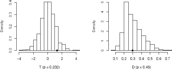
The value of $\widehat{p}$ is the proportion of replicates T* that are at least as large as the observed test statistic (an approximate p-value). For a two-tail test the ASL is 2 $\widehat{p}$ if $\widehat{p}$ ≤ 0.5 (it is 2(1 − $\widehat{p}$) if $\widehat{p}$ > 0.5). The ASL is 0.202 so the null hypothesis is not rejected. For comparison, the two-sample t-test reports p-value = 0.198. A histogram of the replicates of T is displayed by

 hist(reps, main = "", freq = FALSE, xlab = "T (p = 0.202)",

   breaks = "scott")

 points(t0, 0, cex = 1, pch = 16) #observed T

which is shown in Figure 8.1.

8.2 Tests for Equal Distributions

Suppose that X = (X1, ... , Xn) and Y = (Yl, ... , Ym) are independent random samples from distributions F and G respectively, and we wish to test the hypothesis Ho : F = G vs the alternative Hl : F ≠ G. Under the null hypothesis, samples X, Y , and the pooled sample Z = X ∪ Y , are all random samples from the same distribution F. Moreover, under H0, any subset X* of size n from the pooled sample, and its complement Y*, also represent independent random samples from F.

Suppose that $\widehat{\theta }$ is a two-sample statistic that measures the distance in some sense between F and G. Without loss of generality, we can suppose that large values of $\widehat{\theta }$ support the alternative F ≠ G. By the permutation lemma, under the null hypothesis all values of ${\widehat{\theta }}^{*}=\widehat{\theta }\left(X^{*},Y^{*}\right)$ are equally likely. The permutation distribution of ˆθ is given by (8.4), and an exact permutation test or the approximate permutation test procedure given on page 217 can be applied.

Two-sample tests for univariate data

To apply a permutation test of equal distributions, choose a test statistic that measures the difference between two distributions. For example, the two-sample Kolmogorov-Smirnov (K-S) statistic or the two-sample Cramér-von Mises statistic can be applied in the univariate case. Many other statistics are in the literature, although the K-S statistic is one of the most widely applied for univariate distributions. It is applied in the following example.

Example 8.2 (Permutation distribution of the K-S statistic)

In Example 8.1 the means of the soybean and linseed groups were compared. Suppose now that we are interested in testing for any type of difference in the two groups. The hypotheses of interest are H0 : F = G vs H1 : F ≠ G, where F is the distribution of weight of chicks fed soybean supplements and G is the distribution of weight of chicks fed linseed supplements. The Kolmogorov-Smirnov statistic D is the maximum absolute difference between the ecdf’s of the two samples, defined by

$D=\underset{1\le i\le N}{{\displaystyle \sup }}\left|F_n\left(z{}_i\right)-G_m\left(z_i\right)\right|,$

where Fn is the ecdf of the first sample x1, ... , xn and Gm is the ecdf of the second sample y1, ... , ym. Note that 0 ≤ D ≤ 1 and large values of D support the alternative F ≠ G. The observed value of D = D(X,Y) = 0.2976190 can be computed using ks.test. To determine whether this value of D is strong evidence for the alternative, we compare D with the replicates D* = D(X*, Y*).

 R <- 999   #number of replicates

 z <- c(x, y)  #pooled sample

 K <- 1:26

 D <- numeric(R) #storage for replicates

 options(warn = -1)

 D0 <- ks.test(x, y, exact = FALSE)$statistic

 for (i in 1:R) { 

   #generate indices k for the first sample 

   k <- sample(K, size = 14, replace = FALSE)

   x1 <- z[k]

   y1 <- z[-k] #complement of x1

   D[i] <- ks.test(x1, y1, exact = FALSE)$statistic

  }

 p <- mean(c(D0, D) >= D0) 

 options(warn = 0)

 > p

 [1] 0.46

The approximate ASL 0.46 does not support the alternative hypothesis that distributions differ. A histogram of the replicates of D is displayed by

 hist(D, main = "", freq = FALSE, xlab = "D (p = 0.46)",

  breaks = "scott")

 points(D0, 0, cex = 1, pch = 16)  #observed D

which is shown in Figure 8.1.

R note 8.1 In Example 8.2 the Kolmogorov-Smirnov test ks.test generates a warning each time it tries to compute a p-value, because there are ties in the data. We are not using the p-value, so it is safe to ignore these warnings. Display of warnings or messages at the console regarding warnings can be suppressed by options(warn = -1). The default value is warn = 0.

Example 8.3 (Two-sample K-S test)

Test whether the distributions of chick weights for the sunflower and linseed groups differ. The K-S test can be applied as in Example 8.2.

 attach(chickwts)

 x <- sort(as.vector(weight[feed == "sunflower"]))

 y <- sort(as.vector(weight[feed == "linseed"]))

 detach(chickwts)

The sample sizes are n = m = 12, and the observed K-S test statistic is D = 0.8333. The summary statistics below suggest that the distributions of weights for these two groups may differ.

 > summary(cbind(x, y))

  x   y

 Min.  :226.0 Min.  :141.0

 1st Qu.:312.8 1st Qu.:178.0

 Median :328.0 Median :221.0 

 Mean  :328.9 Mean  :218.8

 3rd Qu.:340.2 3rd Qu.:257.8

 Max.  :423.0 Max.  :309.0

Repeating the simulation in Example 8.2 with the sunflower sample replacing the soybean sample produces the following result.

 p <- mean(c(D0, D) >= D0) 

 > p

 [1] 0.001

Thus, none of the replicates are as large as the observed test statistic. Here the sample evidence supports the alternative hypothesis that the distributions differ.

Another univariate test for the two-sample problem is the Cramér-von Mises test [56, 281],. The Cramér-von Mises statistic, which estimates the integrated squared distance between the distributions, is defined by

$W_2=\frac{mn}{{(m+n)}^2}\left[{\displaystyle \sum _{i=1}^n{\left(F_n\left(x_i\right)-G_m(x_i)\right)}^2+}{\displaystyle \sum _{j=1}^n{\left(F_n\left(y_i\right)-G_m(y_i)\right)}^2}\right],$

where Fn is the ecdf of the sample x1, ... , xn and Gm is the ecdf of the sample y1, ... , ym. Large values of W2 are significant. The implementation of the Cramér-von Mises test is left as an exercise.

The multivariate tests discussed in the next section can also be applied for testing H0 : F = G in the univariate case.

8.3 Multivariate Tests for Equal Distributions

Classical approaches to the two-sample problem in the univariate case based on comparing empirical distribution functions, such as the Kolmogorov—Smirnov and Cramér-von Mises tests, do not have a natural distribution free extension to the multivariate case. Multivariate tests based on maximum likelihood depend on distributional assumptions about the underlying populations. Hence although likelihood tests may apply in special cases, they do not apply to the general two-sample or k-sample problem, and may not be robust to departures from these assumptions.

Many of the procedures that are available for the multivariate two-sample problem (8.1) require a computational approach for implementation. Bickel [27] constructed a consistent distribution free multivariate extension of the univariate Smirnov test by conditioning on the pooled sample. Friedman and Rafsky [101] proposed distribution free multivariate generalizations of the Wald-Wolfowitz runs test and Smirnov test for the two-sample problem, based on the minimal spanning tree of the pooled sample. A class of consistent, asymptotically distribution free tests for the multivariate problem is based on nearest neighbors [28, 139, 240]. The nearest neighbor tests apply to testing the k-sample hypothesis when all distributions are continuous. A multivariate nonparametric test for equal distributions was developed independently by Baringhaus and Franz [20] and Székely and Rizzo [261, 262], which is implemented as an approximate permutation test. We will discuss the latter two, the nearest neighbor tests and the energy test [226, 261],.

In the following sections multivariate samples will be denoted by boldface type. Suppose that

$\text{X}=\left\{X_1,\mathrm{...}{X}_{n1}\right\}\in {ℝ}^d,\text{Y=}\left\{Y_1,\mathrm{...}{Y}_{n2}\right\}\in {ℝ}^d,$

are independent random samples, d ≥ 1. The pooled data matrix is Z, an n × d matrix with observations in rows:

$\begin{array}{cc}{\mathbf{\text{z}}}_{n\times d}=\left[\begin{array}{llll}{x}_{1,1}\hfill & x_{1,2}\hfill & \cdots \hfill & x_{1,d}\hfill \\ x_{2,1}\hfill & x_{2,2}\hfill & \cdots \hfill & x_{2,d}\hfill \\ ⋮\hfill & ⋮\hfill & \hfill & ⋮\hfill \\ x_{n_1,1}\hfill & x_{n_1,2}\hfill & \cdots \hfill & x_{n_1,d}\hfill \\ y_{1,1}\hfill & y_{1,2}\hfill & ...\hfill & y_{1,d}\hfill \\ y_{2,1}\hfill & y_{2,2}\hfill & \cdots \hfill & y_{2,d}\hfill \\ ⋮\hfill & ⋮\hfill & \hfill & ⋮\hfill \\ y_{n_2,1}\hfill & y_{n_2,2}\hfill & \cdots \hfill & y_{n_2,d}\hfill \end{array}\right],& (8.5)\end{array}$

where n = n1 + n2.

Nearest neighbor tests

A multivariate test for equal distributions is based on nearest neighbors. The nearest neighbor (NN) tests are a type of test based on ordered distances between sample elements, which can be applied when the distributions are continuous.

Usually the distance is the Euclidean norm $||Z_i-Z_j||$. The NN tests are based on the first through rth nearest neighbor coincidences in the pooled sample. Consider the simplest case, r = 1. For example, if the observed samples are the weights in Example 8.3

  [,1] [,2] [,3] [,4] [,5] [,6] [,7] [,8] [,9] [,10] [,11] [,12]

 x 423 340 392 339 341 226 320 295 334  322  297  318

 y 309 229 181 141  260 203 148 169 213  257  244  271

then the first nearest neighbor of x1 = 423 is x3 = 392, which are in the same sample. The first nearest neighbor of x6 = 226 is y2 = 229, in different samples. In general, if the sampled distributions are equal, then the pooled sample has on average less nearest neighbor coincidences than under the alternative hypothesis. In this example, most of the nearest neighbors are found in the same sample.

Let Z = {X1, ... , Xn1, Y1, ... , Yn2} as in (8.5). Denote the first nearest neighbor of Zi by NN1(Zi). Count the number of first nearest neighbor coincidences by the indicator function Ii(1), which is defined by

$\begin{array}{l}{I}_i\text{(1) = 1 if }{Z}_i\text{ and }N{N}_1(Z_i)\text{ belong to the same sample;}\\ I_i\text{(1) = 0 if }{Z}_i\text{ and }N{N}_1(Z_i)\text{ belong to different samples}\text{.}\end{array}$

The first nearest neighbor statistic is the proportion of first nearest neighbor coincidences

$T_{n,1}=\frac{1}{n}{\displaystyle \sum _{i=1}^n{I}_i\left(1\right)},$

where n = n1 + n2. Large values of Tn,1 support the alternative hypothesis that the distributions differ.

Similarly, denote the second nearest neighbor of a sample element Zi by NN2(Zi) and define the indicator function Ii(2), which is 1 if NN2(Zi) is in the same sample as Zi and otherwise Ii(2) = 0. The second nearest neighbor statistic is based on the first and second nearest neighbor coincidences, defined by

$T_{n,2}=\frac{1}{2n}{\displaystyle \sum _{i=1}^n\left(I_i\left(1\right)+I_i\left(2\right)\right)}.$

In general, the rth nearest neighbor of Zi is defined to be the sample element Zj satisfying $||Z_i-Z_l||<||Z_i-Z_j||$ for exactly r-1 indices 1 ≤ l ≤ n, l ≠ i Denote the rth nearest neighbor of a sample element Zi by NNr(Zi). For i = 1,...,n the indicator function Ii(r) is defined by Ii(r) = 1 if Zi and NNr(Zi) belong to the same sample, and otherwise Ii(r) = 0. The Jth nearest neighbor statistic measures the proportion of first through Jth nearest neighbor coincidences:

$\begin{array}{cc}{T}_{n,J}=\frac{1}{nJ}{\displaystyle \sum _{i=1}^n{\displaystyle \sum _{r=1}^J{I}_i(r)}}.& (8.6)\end{array}$

Under the hypothesis of equal distributions, the pooled sample has on average less nearest neighbor coincidences than under the alternative hypothesis, so the test rejects the null hypothesis for large values of Tn,J. Henze [139] proved that the limiting distribution of a class of nearest neighbor statistics is normal for any distance generated by a norm on ℝd. Schilling [240] derived the mean and variance of the distribution of Tn,2 for selected values of n1/n and d in the case of Euclidean norm. In general, the parameters of the normal distribution may be difficult to obtain analytically. If we condition on the pooled sample to implement an exact permutation test, the procedure is distribution free. The test can be implemented as an approximate permutation test, following the procedure outlined on page 217.

Remark 8.1

Nearest neighbor statistics are functions of the ordered distances between sample elements. The sampled distributions are assumed to be continuous, so there are no ties. Thus, resampling without replacement is the correct resampling method and the permutation test rather than the ordinary bootstrap should be applied. In the ordinary bootstrap, many ties would occur in the bootstrap samples.

Searching for nearest neighbors is not a trivial computational problem, but fast algorithms have been developed [25, 12, 13]. A fast nearest neighbor method nn is available in the knnFinder package. The algorithm uses a kdtree. According to the package author Kemp [160], “The advantage of the kd-tree is that it runs in O(M log M) time ... where M is the number of data points using Bentley’s kd-tree.”

Example 8.4 (Finding nearest neighbors)

The following numerical example illustrates the usage of the nn (knnFinder) [160] function as a method to find the indices of the first through rth nearest neighbors. The pooled data matrix Z is assumed to be in the layout (8.5).

 library(knnFinder) #for nn function

 #generate a small multivariate data set

 x <- matrix(rnorm(12), 3, 4)

 y <- matrix(rnorm(12), 3, 4)

 z <- rbind(x, y) 

 o <- rep(0, nrow(z))

 DATA <- data.frame(cbind(z, o)) 

 NN <- nn(DATA, p = nrow(z)-1)

In the distance matrix below, for example, the first through fifth nearest neighbors of Z1 are Z4, Z2, Z3, Z5, Z6.

 > D <- dist(z)

 > round(as.matrix(D), 2)

  1   2   3   4   5   6

 1 0.00 2.29 2.69 1.88 2.87 3.94

 2 2.29 0.00 2.60 3.27 2.45 3.69

 3 2.69 2.60 0.00 2.14 0.43 3.52

 4 1.88 3.27 2.14 0.00 2.52 3.66

 5 2.87 2.45 0.43 2.52 0.00 3.48

 6 3.94 3.69 3.52 3.66 3.48 0.00

The index matrix returned by the function nn identifies the nearest neighbors as follows. The ith row of $nn.idx on the next page contains the subscripts (indices) of NN1(Zi), NN2(Zi),..., the nearest neighbors of Zi. According to the first row of the index matrix $nn.idx, the indices of the first through fifth nearest neighbors of Z1 are 4, 2, 3, 5, and 6, respectively.

 > NN$nn.idx

  X1 X2 X3 X4 X5

 1  4  2  3  5  6

 2  1  5  3  4  6

 3  5  4  2  1  6

 4  1  3  5  2  6

 5  3  2  4  1  6

 6  5  3  4  2  1

 > round(NN$nn.dist, 2)

   X1  X2  X3  X4  X5

 1 1.88 2.29 2.69 2.87 3.94

 2 2.29 2.45 2.60 3.27 3.69

 3 0.43 2.14 2.60 2.69 3.52

 4 1.88 2.14 2.52 3.27 3.66

 5 0.43 2.45 2.52 2.87 3.48

 6 3.48 3.52 3.66 3.69 3.94

In this small data set it is easy to compute the nearest neighbor statistics. For example, Tn,1 = 2/6 ≐ 0.333 and

$T_{n,2}=\frac{1}{2n}{\displaystyle \sum _{i=1}^n\left(I_i\left(1\right)+I_i\left(2\right)\right)}=\frac{1}{12}\left(2+1\right)=\mathrm{0.25.}$

Example 8.5 (Nearest neighbor statistic)

In this example a method of computing nearest neighbor statistics from the result of nn (knnFinder) is shown. Compute Tn,3 for the chickwts data from Example 8.3.

 library(knnFinder)

 attach(chickwts)

 x <- as.vector(weight[feed == "sunflower"])

 y <- as.vector(weight[feed == "linseed"])

 detach(chickwts)

 z <- c(x, y)

 o <- rep(0, length(z))

 z <- as.data.frame(cbind(z, o))

 NN <- nn(z, p=3)

The data and the index matrix NN$nn.idx are shown on the facing page.

 pooled sample  $nn.idx

  [1,]   X1 X2 X3 

 [1,] 423   1  3  5  2

 [2,] 340   2  4  5  9

 [3,] 392   3  1  5  2

 [4,] 339   4  2  5  9

 [5,] 341   5  2  4  9

 [6,] 226   6  14 21 23

 [7,] 320   7  12 10 13

 [8,] 295   8  11 13 12

 [9,] 334   9  4  2  5

 [10,] 322   10  7 12  9

 [11,] 297   11  8 13 12

 [12,] 318   12  7 10 13 I=1 if index <= 12

 [13,] 309   13 12  7  11 I=1 if index > 12

 [14,] 229   14  6  23  21

 [15,] 181   15 20  18  21

 [16,] 141   16 19  20  15

 [17,] 260   17 22  24  23

 [18,] 203   18 21  15  6

 [19,] 148   19 16  20  15

 [20,] 169   20 15  19  16

 [21,] 213   21 18  6  14

 [22,] 257   22 17  23  24

 [23,] 244   23 22  14  17

 [24,] 271   24 17  22  8

The first three nearest neighbors of each sample element Zi are in the ith row. In the first block, count the number of entries that are between 1 and n1 = 12. In the second block, count the number of entries that are between n1 + 1 = 13 and n1 + n2 = 24.

 block1 <- NN$nn.idx[1:12,]

 block2 <- NN$nn.idx[13:24,]

 i1 <- sum(block1 < 12.5)

 i2 <- sum(block2 > 12.5)

 > c(i1, i2)

 [1] 29 29

Then

$T_{n,3}=\frac{1}{3n}{\displaystyle \sum _{i=1}^n{\displaystyle \sum _{j=1}^3{I}_i(j)=}}\frac{1}{3(24)}(29+29)=\frac{58}{72}=0.8055556.$

Example 8.6 (Nearest neighbor test)

The permutation test for Tn,3 in Example 8.5 can be applied using the boot function in the boot package [34] as follows.

 library(boot)

 Tn3 <- function(z, ix, sizes) {

   n1 <- sizes[1]

   n2 <- sizes[2]

   n <- n1 + n2

   z <- z[ix,]

   o <- rep(0, NROW(z))

   z <- as.data.frame(cbind(z, o))

   NN <- nn(z, p=3)

   block1 <- NN$nn.idx[1:n1,] 

   block2 <- NN$nn.idx[(n1+1):n,]

   i1 <- sum(block1 < n1 + .5)

   i2 <- sum(block2 > n1 + .5)

   return((i1 + i2) / (3 * n))

}

 N <- c(12, 12)

 boot.obj <- boot(data = z, statistic = Tn3,

   sim = "permutation", R = 999, sizes = N)

Note: The permutation samples can also be generated by the sample function. The result of the simulation is

 > boot.obj

 DATA PERMUTATION

 Call: boot(data = z, statistic = Tn3, R = 999,

   sim = "permutation", sizes = N)

 Bootstrap Statistics :

  original bias  std.error

 t1* 0.8055556 -0.3260066 0.07275428

The output from boot does not include a p-value, of course, because boot has no way of knowing what hypotheses are being tested. What is printed at the console is a summary of the boot object. The boot object itself is a list that contains several things including the permutation replicates of the test statistic. The test decision can be obtained from the observed statistic in $t0 and the replicates in $t.

 > tb <- c(boot.obj$t, boot.obj$t0)

 > mean(tb >= boot.obj$t0)

 [1] 0.001

The ASL is $\widehat{p}$ = 0.001, so the hypothesis of equal distributions is rejected. The histogram of replicates of Tn,3 is shown in Figure 8.2.

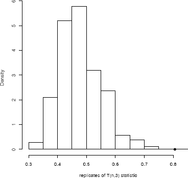
 hist(tb, freq=FALSE, main="",

  xlab="replicates of T(n,3) statistic")

 points(boot.obj$t0, 0, cex=1, pch=16)

The multivariate rth nearest neighbor test can be implemented by an approximate permutation test. The steps are to write a general function that computes the statistic Tn,r for any given (n1, n2, r) and permutation of the row indices of the pooled sample. Then apply boot or generate permutations using sample, similar to the implementation of the permutation test shown in Example 8.6.

Energy test for equal distributions

The energy distance or e-distance statistic εn is defined by

${\epsilon }_n=e\left(X,Y\right)=\frac{n_1{n}_2}{n_1+n_2}\left(\frac{2}{n_1+n_2}{\displaystyle \sum _{i=1}^{n_1}{\displaystyle \sum _{j=1}^{n_2}||X_i-Y_j||}}-\frac{1}{n_1^2}{\displaystyle \sum _{i=1}^{n_1}{\displaystyle \sum _{j=1}^{n_1}||X_i-Y_j||}-\frac{1}{n_2^2}}{\displaystyle \sum _{i=1}^{n_2}{\displaystyle \sum _{j=1}^{n_2}||Y_i-Y_j||}}\right).(8.7)$

On the name “energy” and concept of energy statistics in general see [258, 259],. The non-negativity of e(X,Y) is a special case of the following inequality. If $X,X^{\prime },Y,Y^{\prime }$ are independent random vectors in ℝd with finite expectations, $X\stackrel{D}{=}{X}^{\prime }\text{and}Y\stackrel{D}{=}{Y}^{\prime },$ then

$\begin{array}{cc}2E||X-Y||-E||X-X^{\prime }||-E||Y-Y^{\prime }||\ge 0,& (8.8)\end{array}$

and equality holds if and only if X and Y are identically distributed [262, 263],. The ε distance between the distribution of X and Y is

$\epsilon (X,Y)=2E||X-Y||-E||X-X^{\prime }||-E||Y-Y^{\prime }||$

and the empirical distance εn = e(X,Y) is a constant times the plug-in estimator of ε(X,Y).

Clearly large e-distance corresponds to different distributions, and measures the distance between distributions in a similar sense as the univariate empirical distribution function (edf) statistics. In contrast to edf statistics, however, e-distance does not depend on the notion of a sorted list, and e-distance is by definition a multivariate measure of distance between distributions.

If X and Y are not identically distributed, and n = n1 + n2, then E[εn] is asymptotically a positive constant times n. As the sample size n tends to infinity, under the null hypothesis E[εn] tends to a positive constant, while under the alternative hypothesis E[εn] tends to infinity. Not only the expected value of εn, but εn itself, converges (in distribution) under the null hypothesis, and tends to infinity (stochastically) otherwise. A test for equal distributions based on εn is universally consistent against all alternatives with finite first moments [261, 262]. The asymptotic distribution of εn is a quadratic form of centered Gaussian random variables, with coefficients that depend on the distributions of X and Y .

To implement the test, suppose that Z is the n × d data matrix of the pooled sample as in (8.5). The permutation operation is applied to the row indices of Z. The calculation of the test statistic has O(n2) time complexity, where n = n1 + n2 is the size of the pooled sample. (In the univariate case the statistic can be written as a linear combination of the order statistics, with O(n log n) complexity.)

Example 8.7 (Two-sample energy statistic)

The approximate permutation energy test is implemented in eqdist.etest in the energy package [226]. However, in order to illustrate the details of the implementation for a multivariate permutation test, we provide an R version below. Note that the energy implementation is considerably faster than the example below, because in eqdist.etest the calculation of the test statistic is implemented in an external C library.

The εn statistic is a function of the pairwise distances between sample elements. The distances remain invariant under any permutation of the indices, so it is not necessary to recalculate distances for each permutation sample.

However, it is necessary to provide a method for looking up the correct distance in the original distance matrix given the permutation of indices.

 edist.2 <- function(x, ix, sizes) {

   # computes the e-statistic between 2 samples

   # x:  Euclidean distances of pooled sample

   # sizes:  vector of sample sizes

   # ix:  a permutation of row indices of x

   dst <- x

   n1 <- sizes[1]

   n2 <- sizes[2]

   ii <- ix[1:n1]

   jj <- ix[(n1+1):(n1+n2)]

   w <- n1 * n2 / (n1 + n2)

   # permutation applied to rows & cols of dist. matrix

   m11 <- sum(dst[ii, ii]) / (n1 * n1)

   m22 <- sum(dst[jj, jj]) / (n2 * n2)

   m12 <- sum(dst[ii, jj]) / (n1 * n2) 

   e <- w * ((m12 + m12) - (m11 + m22))

   return (e)

}

Below, the simulated samples in ℝd are generated from distributions that differ in location. The first distribution is centered at μ1 = (0, ... , 0)T and the second distribution is centered at μ2 = (a,... , a)T .

 d <- 3

 a <- 2 / sqrt(d)

 x <- matrix(rnorm(20 * d), nrow = 20, ncol = d)

 y <- matrix(rnorm(10 * d, a, 1), nrow = 10, ncol = d)

 z <- rbind(x, y)

 dst <- as.matrix(dist(z))

 > edist.2(dst, 1:30, sizes = c(20, 10)) 

 [1] 9.61246

The observed value of the test statistic is εn = 9.61246.

The function edist.2 is designed to be used with the boot (boot) function [34] to perform the permutation test. Alternately, generate the permutation vectors ix using the sample function. The boot method is shown in the following example.

Example 8.8 (Two-sample energy test)

This example shows how to apply the boot function to perform an approximate permutation test using a multivariate test statistic function. Apply the permutation test to the data matrix z in Example 8.7.

 library(boot) #for boot function

 dst <- as.matrix(dist(z)) 

 N <- c(20, 10)

 boot.obj <- boot(data = dst, statistic = edist.2,

   sim = "permutation", R = 999, sizes = N)

 > boot.obj

 DATA PERMUTATION

 Call: boot(data = dst, statistic = edist.2, R = 999,

   sim = "permutation", sizes = N)

 Bootstrap Statistics :

   original  bias std. error

 t1* 9.61246 -7.286621 1.025068

The permutation vectors generated by boot will have the same length as the data argument. If data is a vector then the permutation vector generated by boot will have length equal to the data vector. If data is a matrix, then the permutation vector will have length equal to the number of rows of the matrix. For this reason, it is necessary to convert the dist object to an n × n distance matrix.

The ASL is computed from the replicates in the bootstrap object.

 e <- boot.obj$t0

 tb <- c(e, boot.obj$t)

 mean(tb >= e)

 [1] 0.001

 hist(tb, main = "", breaks="scott", freq=FALSE,

   xlab="Replicates of e") 

 points(e, 0, cex=1, pch=16)

None of the replicates exceed the observed value 9.61246 of the test statistic. The approximate achieved significance level is 0.001, and we reject the hypothesis of equal distributions. Replicates of εn, are shown in Figure 8.3(a).

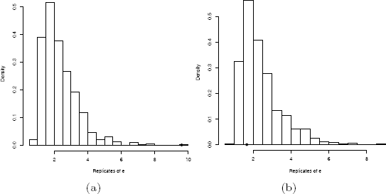
The large estimate of bias reported by the boot function gives an indication that the test statistic is large, because ε(X,Y) ≥ 0 and ε(X,Y) = 0 if and only if the sampled distributions are equal.

Finally, let us check the result of the test when the sampled distributions are identical.

 d <- 3

 a <- 0

 x <- matrix(rnorm(20 * d), nrow = 20, ncol = d)

 y <- matrix(rnorm(10 * d, a, 1), nrow = 10, ncol = d)

 z <- rbind(x, y)

 dst <- as.matrix(dist(z))

 N <- c(20, 10)

 dst <- as.matrix(dist(z))

 boot.obj <- boot(data = dst, statistic = edist.2, 

   sim="permutation", R=999, sizes=N)

 > boot.obj

 ...

 Bootstrap Statistics :

   original bias std. error

 t1* 1.664265 0.7325929 1.051064

 e <- boot.obj$t0

 E <- c(boot.obj$t, e)

 mean(E >= e)

[1] 0.742

 hist(E, main = "", breaks="scott",

   xlab="Replicates of e", freq=FALSE) 

 points(e, 0, cex=1, pch=16)

In the second example the approximate achieved significance level is 0.742 and the hypothesis of equal distributions is not rejected. Notice that the estimate of bias here is small. The histogram of replicates is shown in Figure 8.3(b).

The ε; distance and two-sample e-statistic εn are easily generalized to the k-sample problem. See e.g. the function edist (energy), which returns a dissimilarity object like the dist object.

Example 8.9 (k-sample energy distances)

The function edist.2 in Example 8.7 is a two-sample version of the function edist in the energy package [226], which summarizes the empirical ε-distances between k ≥ 2 samples. The syntax is

 edist(x, sizes, distance=FALSE, ix=1:sum(sizes), alpha=1)

The argument alpha is an exponent 0 < α ≤ 2 on the Euclidean distance.

234It can be shown that for all 0 < α < 2 the corresponding e(α)-distance determines a statistically consistent test of equal distributions for all random vectors with finite first moments [262].

Consider the four-dimensional iris data. Compute the e-distance matrix for the three species of iris.

 library(energy) #for edist

 z <- iris[, 1:4]

 dst <- dist(z)

 > edist(dst, sizes = c(50, 50, 50), distance = TRUE)

   1  2

 2 123.55381

 3 195.30396 38.85415

A test for the k-sample hypothesis of equal distributions is based on k-sample e-distances with a suitable weight function.

Comparison of nearest neighbor and energy tests

Example 8.10 (Power comparison)

In a simulation experiment, we compared the empirical power of the third nearest neighbor test based on Tn,3 (8.6) and the energy test based on εn (8.7). The distributions compared,

$\begin{array}{cc}{F}_1=N_2\left(\mu ={\left(0,0\right)}^2,{\displaystyle \sum \text{ }=I_2}\right),& F_2=N_2\left(\mu ={\left(0,\delta \right)}^T,{\displaystyle \sum \text{ }}=I_2\right),\end{array}$

differ in location. The empirical power was estimated for δ = 0, 0.5, 0.75, 1, from a simulation of permutation tests on 10, 000 pairs of samples. Each permutation test decision was based on 499 permutation replicates (each entry in the table required 5 · 106 calculations of the test statistic). Empirical results are given below for selected alternatives, sample sizes, and dimension, at significance level a = 0.1. Both the εn and Tn,3 statistics achieved approximately correct empirical significance in our simulations (see case δ = 0 in Table 8.1), although the Type I error rate for Tn,3 may be slightly inflated when n is small.

These alternatives differ in location only, and the empirical evidence summarized in Table 8.1 suggests that εn is more powerful than Tn,3 against this class of alternatives.

8.4 Application: Distance Correlation

A test of independence of random vectors X ∈ ℝp and Y ∈ ℝq

$\begin{array}{ccc}{H}_0:F_{XY}=F_X{F}_Y& vs& H_1:F_{XY}\ne F_X{F}_Y\end{array}$

can be implemented as a permutation test. The permutation test does not require distributional assumptions, or any type of model specification for the dependence structure. Not many universally consistent nonparametric tests exist for the general hypothesis above. In this section we will discuss a new multivariate nonparametric test of independence based on distance correlation [265] that is consistent against all dependent alternatives with finite first moments. The test will be implemented as a permutation test.

Distance Correlation

Distance correlation is a new measure of dependence between random vectors introduced by Székely, Rizzo, and Bakirov [265]. For all distributions with finite first moments, distance correlation $\mathcal{R}$ generalizes the idea of correlation in two fundamental ways:

1. $ℛ\left(X,Y\right)$ is defined for X and Y in arbitrary dimension.
2. $ℛ\left(X,Y\right)=0$ characterizes independence of X and Y.

Distance correlation satisfies $0\le ℛ\le 1,andℛ=0$ only if X and Y are independent. Distance covariance $V$ provides a new approach to the problem of testing the joint independence of random vectors. The formal definitions of the population coefficients $V$ and $ℛ$ are given in [265]. The definitions of the empirical coefficients are as follows.

Definition 8.1

The empirical distance covariance $V_n\left(\mathbf{\text{X, Y}}\right)$is the nonnegative number defined by

$\begin{array}{cc}{V}_n^2(\mathbf{\text{X}},\mathbf{\text{Y}})=\frac{1}{n^2}{\displaystyle \sum _{k,l=1}^n{A}_{kl}{B}_{kl},}& (8.9)\end{array}$

where Akl and Bkl are defined in equations (8.11-8.12) below. Similarly, $V_n\left(\mathbf{\text{X}}\right)$ is the nonnegative number defined by

$\begin{array}{cc}{V}_n^2(\mathbf{\text{X}})=V_n^2(\mathbf{\text{X,Y}})=\frac{1}{n^2}{\displaystyle \sum }_{k,l=1}^n{A}_{kl}^2.& (8.10)\end{array}$

The formulas for Akl and Bkl in (8.9–8.10) are given by

$\begin{array}{cc}{A}_{kl}=a_{kl}-{\overline{a}}_{k.}-{\overline{a}}_{.l}+\overline{a}\mathrm{..};& (8.11)\end{array}$

$\begin{array}{cc}{B}_{kl}=b_{kl}-{\overline{b}}_{k.}-{\overline{b}}_{.l}+\overline{b}\mathrm{..},& (8.12)\end{array}$

where

$\begin{array}{ccc}{a}_{kl}=||X_k-X_l||\mathrm{p,}& b_{kl}=||Y_k-Y_l||q,& k,l=1,\mathrm{...},n,\end{array}$

and the subscript “.” denotes that the mean is computed for the index that it replaces. Note that these formulas are similar to computing formulas in analysis of variance, so the distance covariance statistic is very easy to compute. Although it may not be obvious that $V_n^2\left(\mathbf{\text{X,Y}}\right)\ge 0,$, this fact as well as the motivation for the definition of $\mathcal{V}$ is explained in [265].

Definition 8.2

The empirical distance correlation Rn(X,Y) is the square root of

$\begin{array}{cc}{ℛ}_n^2\left(\mathbf{\text{X,Y}}\right)=\{\begin{array}{cc}\frac{{\mathcal{V}}_n^2(\mathbf{X},\mathbf{Y})}{\sqrt{{\mathcal{V}}_n^2(\mathbf{X}),{\mathcal{V}}_n^2(\mathbf{Y})}},& {\mathcal{V}}_n^2(\mathbf{X}),{\mathcal{V}}_n^2(\mathbf{Y})>0;\\ 0,& {\mathcal{V}}_n^2(\mathbf{X}),{\mathcal{V}}_n^2(\mathbf{Y})=0.\end{array}& (8.13)\end{array}$

The asymptotic distribution of $n{\mathcal{V}}_n^2$ is a quadratic form of centered Gaussian random variables, with coefficients that depend on the distributions of X and Y. For the general problem of testing independence when the distributions of X and Y are unknown, the test based on $n{\mathcal{V}}_n^2$ can be implemented as a permutation test.

Before proceeding to the details of the permutation test, we implement the calculation of the distance covariance statistic (dCov).

Example 8.11 (Distance covariance statistic)

In the distance covariance function dCov, operations on the rows and columns of the distance matrix generate the matrix with entries Akl. Note that each term

$A_{kl}=a_{kl}-{\overline{a}}_{k.}-{\overline{a}}_{.l}+\overline{a}\mathrm{..};a_{kl}=||X_k-X_l||$

is a function of the distance matrix of the X sample. In the function Akl, the sweep operator is used twice. The first sweep subtracts a. l, the row means, from the distances akl. The second sweep subtracts ak., the column means, from the result of the first sweep. (The column means and row means are equal because the distance matrix is symmetric.) If the samples are x and y, then the matrix A = (Akl) is returned by Akl(x) and the matrix B = (Bkl) is returned by Akl(y). The remaining calculations are simple functions of these two matrices.

 dCov <- function(x, y) {

   x <- as.matrix(x)

   y <- as.matrix(y)

   n <- nrow(x)

   m <- nrow(y)

   if (n != m || n < 2) stop("Sample sizes must agree")

   if (! (all(is.finite(c(x, y)))))

   stop("Data contains missing or infinite values")

   Akl <- function(x) {

   d <- as.matrix(dist(x))

   m <- rowMeans(d)

   M <- mean(d)

   a <- sweep(d, 1, m)

   b <- sweep(a, 2, m)

   return(b + M)

}

 A <- Akl(x)

 B <- Akl(y)

 dCov <- sqrt(mean(A * B))

 dCov

}

A simple example to try out the dCov function is the following. Compute ${\mathcal{V}}_n$ for the bivariate distributions of iris setosa (petal length, petal width) and (sepal length, sepal width).

 z <- as.matrix(iris[1:50, 1:4])

 x <- z[, 1:2]

 y <- z[, 3:4]

 # compute the observed statistic

 > dCov(x, y)

 [1] 0.06436159

The returned value is ${\mathcal{V}}_n=\text{0}\text{.06436159}\text{.}$ Here n = 50 so the test statistic for a test of independence is $n{\mathcal{V}}_n^2\doteq 0.207$.

Example 8.12 (Distance correlation statistic)

The distance covariance must be computed to get the distance correlation statistic. Rather than call the distance covariance function three times, which means repeated calculation of the distances and the A and B matrices, it is more efficient to combine all operations in one function.

 DCOR <- function(x, y) {

  x <- as.matrix(x)

  y <- as.matrix(y)

  n <- nrow(x)

  m <- nrow(y)

  if (n != m || n < 2) stop("Sample sizes must agree")

  if (! (all(is.finite(c(x, y)))))

    stop("Data contains missing or infinite values")

  Akl <- function(x) {

    d <- as.matrix(dist(x))

    m <- rowMeans(d)

    M <- mean(d)

    a <- sweep(d, 1, m)

    b <- sweep(a, 2, m)

    return(b + M)

 }

  A <- Akl(x)

  B <- Akl(y)

  dCov <- sqrt(mean(A * B))

  dVarX <- sqrt(mean(A * A))

  dVarY <- sqrt(mean(B * B))

  dCor <- sqrt(dCov / sqrt(dVarX * dVarY))

  list(dCov=dCov, dCor=dCor, dVarX=dVarX, dVarY=dVarY)

}

Applying the function DCOR to the iris data we obtain all of the distance dependence statistics in one step.

 z <- as.matrix(iris[1:50, 1:4])

 x <- z[, 1:2]

 y <- z[, 3:4]

 > unlist(DCOR(x, y))

  dCov  dCor  dVarX  dVarY

 0.06436159 0.61507138 0.28303069 0.10226284

Permutation tests of independence

A permutation test of independence is implemented as follows. Suppose that X ∈ ℝp and Y ∈ ℝq and Z = (X, Y). Then Z is a random vector in ℝp+q. In the following, we suppose that a random sample is in an n × (p + q) data matrix Z with observations in rows:

${\mathbf{Z}}_{n\times d}=\left[\begin{array}{cccccccc}{x}_{1,1}& x_{1,2}& \cdots & x_{1,p}& y_{1,1}& y_{1,2}& \cdots & y_{1,q}\\ x_{2,1}& x_{2,2}& \cdots & x_{2,p}& y_{2,1}& y_{2,2}& \cdots & y_{2,q}\\ ⋮& ⋮& & ⋮& & & & \\ x_{n,1}& x_{n,2}& \cdots & x_{n,p}& y_{n,1}& y_{n,2}& \cdots & x_{n,q}\end{array}\right].$

Let ν1 be the row labels of the X sample and let ν2 be the row labels of the Y sample. Then (Z, ν1, ν2) is the sample from the joint distribution of X and Y . If X and Y are dependent, the samples must be paired and the ordering of labels ν2 cannot be changed independently of ν1. Under independence, the samples X and Y need not be matched. Any permutation of the row labels of the X or Y sample generates a permutation replicate. The permutation test procedure for independence permutes the row indices of one of the samples (it is not necessary to permute both ν1 and ν2).

Approximate permutation test procedure for independence

Let $\widehat{\theta }$ be a two sample statistic for testing multivariate independence.

1. Compute the observed test statistic $\widehat{\theta }\left(X,Y\right)=\widehat{\theta }\left(Z,v_1,v_2\right).$
2. For each replicate, indexed b = 1, ... , B:
   1. Generate a random permutation πb = π(ν2).
   2. Compute the statistic ${\widehat{\theta }}^{\left(b\right)}=\widehat{\theta }*\left(Z,{\pi }_b\right)=\widehat{\theta }\left(X,Y*,\pi \left(v_2\right)\right).$
3. If large values of $\widehat{\theta }$ support the alternative, compute the ASL by

   $\widehat{p}=\frac{1+\#\left\{{\widehat{\theta }}^{\left(b\right)}\ge \widehat{\theta }\right\}}{B+1}=\frac{\left\{1+{\displaystyle {\sum }_{b=1}^{B}I\left({\widehat{\theta }}^{\left(b\right)}\ge \widehat{\theta }\right)}\right\}}{B+1}.$

   The ASL for a lower-tail or two-tail test based on $\widehat{\theta }$ is computed in a similar way.

4. Reject H0 at significance level a if $\widehat{p}\le \alpha .$

Example 8.13 (Distance covariance test)

This example tests whether the bivariate distributions (petal length, petal width) and (sepal length, sepal width) of iris setosa are independent. To implement a permutation test, write a function to compute the replicates of the test statistic $n{\mathcal{V}}_n^2$ that takes as its first argument the data matrix and as its second argument the permutation vector.

 ndCov2 <- function(z, ix, dims) {

   #dims contains dimensions of x and y

   p <- dims[1]

   q1 <- dims[2] + 1

   d <- p + dims[2]

   x <- z[, 1:p]  #leave x as is

   y <- z[ix, q1:d] #permute rows of y

   return(nrow(z) * dCov(x, y)^2)

}

 library(boot)

 z <- as.matrix(iris[1:50, 1:4])

 boot.obj <- boot(data = z, statistic = ndCov2, R = 999,

   sim = "permutation", dims = c(2, 2))

 tb <- c(boot.obj$t0, boot.obj$t)

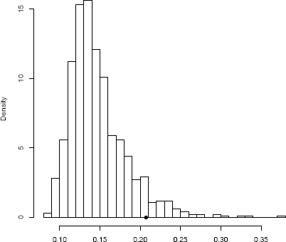
 hist(tb, nclass="scott", xlab="", main="",

   freq=FALSE)

 points(boot.obj$t0, 0, cex=1, pch=16)

 > mean(tb >= boot.obj$t0)

 [1] 0.066

 > boot.obj

 DATA PERMUTATION

 Call: boot(data = z, statistic = ndCov2, R = 999,

  sim = "permutation", dims = c(2, 2))

 Bootstrap Statistics :

   original  bias std.error

 t1* 0.2071207 -0.05991699 0.0353751

The achieved significance level is 0.066 so the null hypothesis of independence is rejected at α = 0.10. The histogram of replicates of the dCov statistic is shown in Figure 8.4.

One of the advantages of the dCov test is that it is sensitive to all types of dependence structures in data. Procedures based on the classical definition of covariance, or measures of association based on ranks are generally less effective against non-monotone types of dependence. An alternative with non-monotone dependence is tested in the following example.

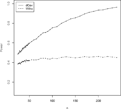
Example 8.14 (Power of dCov)

Consider the data generated by the following nonlinear model. Suppose that

$Y_{ij}=X_{ij}{\epsilon }_{ij},i=1,\text{...},n,j=1,\text{...},5,$

where X ~ N5(0, I5) and ɛ ~ N5(0, σ2I5) are independent. Then X and Y are dependent, but if the parameter σ is large, the dependence can be hard to detect. We compared the permutation test implementation of dCov with the parametric Wilks Lambda (W) likelihood ratio test [296] using Bartlett’s approximation for the critical value (see e.g. [188, Sec. 5.3.2b]). Recall that Wilks Lambda tests whether the covariance Σ12 = Cov(X, Y) is the zero matrix.

From a power comparison with 10,000 test decisions for each of the sample sizes we have obtained the results shown in Table 8.2 and Figure 8.5. Figure 8.5 shows a plot of power vs sample size. Table 8.2 reports the empirical power for a subset of the cases in the plot.

The dCov test is clearly more powerful in this empirical comparison. This example illustrates that the parametric Wilks Lambda test based on product-moment correlation is not always powerful against non-monotone types of dependence. The dCov test is statistically consistent with power approaching 1 as n →∞ (theoretically and empirically).

For properties of distance covariance and distance correlation, proofs of convergence and consistency, and more empirical results, see [265]. The distance correlation and covariance statistics and the corresponding permutation tests are provided in the energy package [226].

Exercises

1. 8.1 Implement the two-sample Cramér-von Mises test for equal distributions as a permutation test. Apply the test to the data in Examples 8.1 and 8.2.

2. 8.2 Implement the bivariate Spearman rank correlation test for independence [255] as a permutation test. The Spearman rank correlation test statistic can be obtained from function cor with method = “spearman”. Compare the achieved significance level of the permutation test with the p-value reported by cor.test on the same samples.

3. 8.3 The Count 5 test for equal variances in Section 6.4 is based on the maximum number of extreme points. Example 6.15 shows that the Count 5 criterion is not applicable for unequal sample sizes. Implement a permutation test for equal variance based on the maximum number of extreme points that applies when sample sizes are not necessarily equal.

4. 8.4 Complete the steps to implement a rth-nearest neighbors test for equal distributions. Write a function to compute the test statistic. The function should take the data matrix as its first argument, and an index vector as the second argument. The number of nearest neighbors r should follow the index argument.

Projects

1. 8.A Replicate the power comparison in Example 8.10, reducing the number of permutation tests from 10000 to 2000 and number of replicates from 499 to 199. Use the eqdist.etest (energy) version of the energy test.

2. 8.B The aml (boot) [34] data contains estimates of the times to remission for two groups of patients with acute myelogenous leukaemia (AML). One group received maintenance chemotherapy treament and the other group did not. See the description in the aml data help topic. Following Davison and Hinkley [63, Example 4.12], compute the log-rank statistic and apply a permutation test procedure to test whether the survival distributions of the two groups are equal.