Chapter 2
Risk Management
In this book, we are going to discuss the ins and outs of risk management. When we talk about managing risks, we are talking about understanding the risk of the positions you take, evaluating them to make sure they are within your policy guidelines, and being able to react to situations that go bad. Risk management is one of the most important keys to trading. Before you start a process of risk management you need to understand the pieces that make up risk management. The key is to understand what the facets of Greek management are that allow a trader to manage a position. This means that a trader has to understand the Greeks at a definitive level:
–Delta represents the position’s sensitivity to changes in an underlying’s change in price. A long delta position wants the underlying to rally. A negative (short) delta position profits from a fall in the underlying.
–Gamma indicates how the position’s delta changes as the underlying moves in one direction or the other. It is often viewed as the rate of change of delta, or mathematically, the slope of the delta curve. Positive gamma will see delta increase if the underlying rallies and fall if the underlying drops. Negative gamma positions will see delta increase as the underlying drops and delta fall as the underlying rallies.
–Vega is a measure of how the position makes or loses money as IV changes. If IV changes 1 point, how does the position behave? Does it make money or lose money? A long vega position will profit from an increase in IV, and a short vega position will lose money if IV increases. Similarly, a long vega position will lose if there is a decrease in IV and a short vega position will profit from an increase in IV.
–Theta represents how a position makes or loses money as time passes. With the passing of each day, how much is the trader making or losing by carrying the current position? Long theta means that as time passes the trader is theoretically making money. Short theta means that there is a daily cost to carrying the current position that can theoretically cost the trader money. But is that it? The answer is no. The key to risk is to understand how these Greeks and the associated risks change as volatility changes. Volatility changes the outputs of risk control and to really be in control of risk, you have to get how these inputs really work . . . not just what they mean.
The Pricing Model
The pricing model for options has five main inputs. While options have been around for 45 years now, the main pieces of the pricing model have never changed. It does not matter whether the firm is Citadel, the leader in advanced option trades, or the average retail trader glued to the screen of a rudimentary brokerage platform. These five factors determine how a trader approaches options:
–Price of the underlying
–Strike price
–Time to expiration
–Cost of carry. For most options trading the cost of carrying is a consideration for levels of dividends (on long positions) or, if margin is used for long positions, the obligation to pay interest.
–Volatility
It is key that you understand what you assume when trading options and use the Greeks to manage your risk—especially for the retail trader, where often the Greeks are set to change with the price of options. While the average market maker can quickly recognize changes in pricing, the standard retail trader cannot. This is because market makers’ lives revolve around volatility and staring at screens. A market maker makes money by trading small changes in volatility up and down and against each other. The retail trader has neither the will nor volition to stare at a screen. Additionally, market makers tend to have better analytics, making their task easier. That is not an excuse, just a firm understanding of how volatility behaves with changes in the five Greeks. This is why a trade wins or loses. In the pages that follow, I’m going to spend some time really describing the Greeks. Please refer to Appendix A for brief descriptions of each of the Greeks.
Delta
Delta is the change in price of an option as the underlying price changes. Thus, if an ATM option (at the money, usually the most actively traded) has a delta of .50, it will gain 50 cents for every dollar the underlying asset rallies. It will lose 50 cents for every dollar the underlying asset falls. Delta, in most platforms, is a dynamic measure, and can move, not just end of day, but as the day moves along (the change is determined by gamma, discussed in the next section).
We will look at delta in a vacuum. If Option XYZ is trading at 2.50 (in options trader lingo, “trading 2.50”) and the underlying XYZ currently trades at $35 per share; XYZ then drops to $34, so option XYZ will be worth 2.00. So, option XYZ would be valued at a lower level per contract if the underlying XYZ fell, with changes reflected point-for-point when ATM.
If Option XYZ is trading at 2.50 and underlying XYZ is trading at $35 and then rallies to $36, option XYZ will be worth 3.00 per contract. If delta was .60, the options would gain 60 cents and would be worth 3.10 on a 1 dollar rally; if .70 it would be worth 3.20 and so on. This is true regardless the size of the contract.
A negative delta will act the opposite way. If the option has a negative delta, it will make money when the underlying falls and lose money when the underlying rallies. In the example above the option would fall to 2.00 on a .50 negative delta option and 1.90 on a .60 negative delta option, etc.
Delta does not care about the underlying price, but relies on the multiplier, how much of the physical underlying each contract expires into. Most options are a 100 multiplier. However, there are a few options that have smaller and larger multipliers, especially in futures options. In the S&P 500 E-mini options, the multiplier is 50 not 100. So, an option would only gain 50 * .50 in our example above. The big S&P options have a multiplier of 250, and an option gains 1.25 on a 1.00 move. The calculation for dollars gained or lost is:
multiplier * delta
I also use delta as a loose interpretation of percentage chance that an option ends up in the money. Understanding the likelihood of a position moving in the money is valuable when setting up a directional trade.
Do I want a trade that looks for a small move or a large move? If I want a large move, I’ll play for a homerun using a low percentage option (low delta). If I expect a smaller move but have some certainty, I move toward a higher delta option to play the percentage. Thus a .60 delta option has a 55–65% chance of ending up in the money, close enough for estimation when doing math in your head, but nothing that should ever be used to directly manage risk.
Seems pretty simple, the concept of delta, but is that it? No, delta is a malleable risk measure that can change. Other factors that affect delta are discussed below. As conditions change in the market, delta changes with the 5 factors that make up the pricing model.
Change in Underlying Price
Some of the factors that move delta are easy to understand and are interrelated with other Greeks. Change in underlying price is the most notable. If I buy a call option that is .50 delta at the $50 strike and the underlying XYZ is trading at $50 per share, then the next week, XYZ moves from $50 to $75 per share, there is no way that delta stays at .50, even in the craziest of market situations. An option that was the same price of the underlying that is now 25 points in the money, even in a large cap stock or index, inherently has different odds of being in the money. Think of this like a basketball game. If teams are tied early on and one team takes a 10 point lead, the odds of the team winning with a 10 point lead must increase even if the game is early on. As the underlying price rallies on a positive delta option, the option’s delta MUST rise. As the underlying falls, delta must change, in this case lower (as we will see, gamma measures this risk).
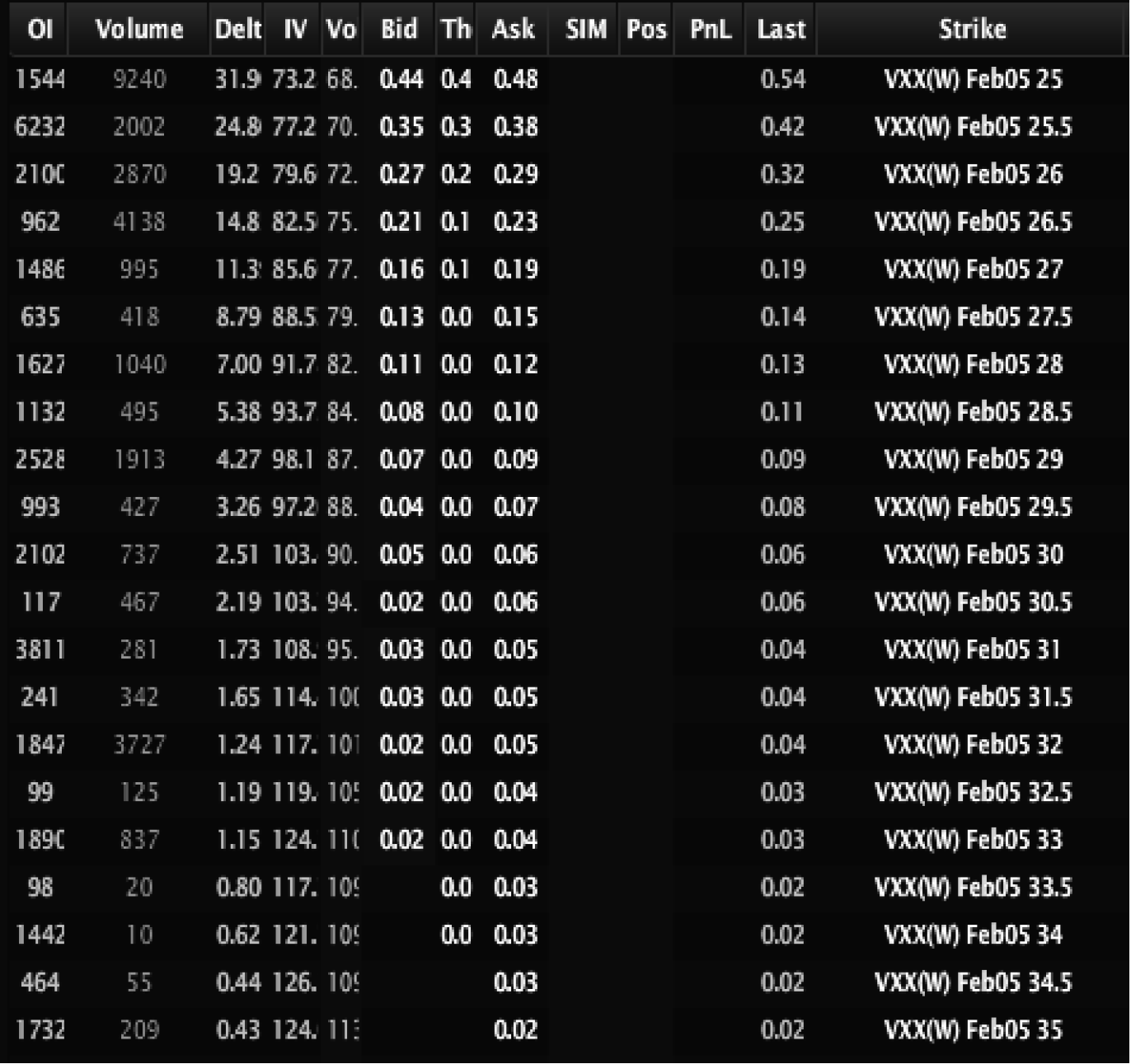
When delta is negative, the opposite holds true. When the underlying rallies, the option will become less negative delta. A quick way to view how delta will change is to look at a montage. Take the example in VIX options shown in Figure 2.1:

Currently VIX March futures are trading at 23. This screen shows the current deltas for strike prices of 20 to 30. It looks good for making the 20 strike, and that is reflected in the high delta. But as you get to 30 for the strike, the chances are slim and the delta is low. If, in the future, it was to run to 25, in theory the VIX 23 option at 2.80 would have a similar delta to the current 21 strike at 3.50 and the 25 strike at 2.20 should be similar to 23 strike at 2.80, and so on. There are other pieces that affect delta, but one way to see how delta moves is to see the deltas at different strikes.
Change in Strike Price
As the strike changes, so changes the delta of the option. The further from ATM (at the money) the underlying is, the further it will be from delta. Looking at VIX options, refer to the montage in Figure 2.1. With the futures trading 23 in March, the 23 strike in VIX is about a .50 delta (.54 delta to be exact). The 20 is a .70 delta and the 30 strike call is a .30 delta option.
This interaction should be intuitive. Strike prices represent whether the option is in the money, out of the money, or at the money. Of all the facets that affect delta, this one is by far the easiest.
Time to Expiration
The more time it takes for a scenario to occur, the more likely that scenario is to happen. Think about it this way: There is almost no way that the average person is going to stop using Facebook in 2016 or 2017. In 2025, it is entirely possible that no one will use Facebook as a social media outlet. Think I am talking crazy? Remember Myspace had 350 million users at one time.
Let’s say AAPL is trading at $150 per share. Could it trade at $200 in 6 months? Probably not. What about a year after it’s published? Maybe? What about two years after its published? Entirely possible. The point is, especially with stocks, the longer it takes for something to occur, the more likely something is to happen. Thus, the AAPL 200 call will have a low delta when there is little time to expiration, but in LEAPS (Long-term Equity AnticiPation Securities) it could have a decently high delta.
Volatility
Volatility is the X factor across all Greeks. I am going to spend a lot of time talking about volatility in this book. A simple way to think about the volatility of the option is that it changes time. As volatility rises, it makes certain scenarios more and more likely to occur, because it points toward large swings in the underlying. As volatility falls, it points toward different scenarios being less likely to happen.
As volatility rises, it predicts greater movement to follow. Considering volatility is annualized—just looking at an annual move, a $1,000 stock with an implied volatility (IV) of 20% expects the underlying to move higher or lower by 200 points with one standard deviation of confidence. If that $1,000 stock sees its IV increase to 25%, the market now expects a move of 250 points per year, regardless of direction. Since volatility is a function of standard deviation, a stock with a volatility of 16% should move about 1% a day (as the square root of 252 is actually 15.87 which would really be 1%).
The calculation for figuring the standard deviation that the market is currently pricing is:
Underlying price * Implied volatility of the AMT strike * SQRT(trading days to expiration/trading days in a year).
Thus, if XYZ is trading at 20 with IV of 16%, the options market is expecting the underlying to move about .20 a day. A 25 strike call with 30 days to expire is unlikely to end up in the money even if the underlying rallies its volatility number every day.
20 * .16 * SQRT(21/252) = .20
Remember: 30 days to expire means about 21 days of trading, so the market looks for about 3.20 of movement if the underlying went straight up over the period of a year.
20 * .16 * SQRT(252/252) = 3.20
Looking at actual volatility over that period of time, taking movement both up and down into consideration, the market is pricing in an XYZ move of 92.
20 * .16 * SQRT(21/252) = .92
The 25’s are not expected to end up in the money. They will end up with a ballpark delta of less than 10 and a value of less than .20 per contract given the current time to expiration.
If expectation of movements increases in stock XYZ to 32%, double that of the previous example, all of the sudden the market is looking for 1.84 over a month of movement and if the stock catches some momentum, the underlying could blow through the upside call. Whereas the 25 strike call had a delta of less than 10 and a value less than .20, the option now has new life. The option will have a delta near 20 and a value near .50 per contract. If the IV jumps to 48%, the strike is going to have some serious value. Delta will be over 25 and the option will start to approach at least a 1.00 valuation give or take (.5 * 2x IV).
The view of volatility is much like turning the clock back. A two-year scenario makes outcomes seem more likely to happen, and higher volatility makes scenarios more likely to happen. If I move IV from 16% to 32%, it’s like moving days to expiration from 30 (21 days to expiration) to 90 days (63 days to expiration) to expiration. To compare:
20 * .16 * SQRT(63/252) = 1.84
20 * .32 * SQRT(21/252) = 1.91
The above are similar even though the days to expiration are different; this is the power volatility has on standard deviation, which determines delta. Nothing will affect the outcome of an option like volatility. To understand a Greek is to understand the effect of volatility.
Gamma
In my experience, gamma is the Greek that traders have the hardest time understanding. It’s also the Greek most likely to blow the trader up. I can speak from experience; there is no trader that has not been beaten badly by gamma. I have had occasions where an explosion in gamma has made or lost thousands of dollars.
Gamma represents how delta changes with a 1 dollar change in the underlying, regardless of the price of the underlying. Thus, if you trade SPX which is about 2000 dollars per contract, gamma measures change in delta for 1 dollar and the same is true if you are trading SPY which is around 200 dollars. Both are indexes of the Standard and Poor’s 500 and yet they have quite different gammas because of the underlying. More importantly, the sign and movement of gamma has nothing to do with the delta value. A negative delta can be accompanied by a positive gamma and a positive delta can have a negative gamma.
Let’s quickly examine gamma:
XYZ is trading at $30, and a long 30 strike put has a negative delta of -0.5 and a positive gamma of 0.1. If the underlying rallies 1 dollar to $31, the delta will change from -0.5 to -0.4.
XYZ is trading $30, and a long 30 strike call has a positive delta of 0.5 and a positive gamma of 0.1. If the underlying rallies 1 to $31 the delta will change from 0.5 to 0.6.
The sign of gamma does not matter. Looking at the opposite:
XYZ is trading at $30, and a short 30 strike put has a negative delta of -0.5 and a positive gamma of 0.1. If the underlying rallies 1 dollar to $31 the delta will change from -0.5 to -0.4.
XYZ is trading at $30, and a short 30 strike call has a positive delta of 0.5 and a positive gamma of 0.1. If the underlying rallies 1 to $31 the delta will change from 0.5 to 0.6.
This is all well and good. Where gamma becomes dangerous is on a gap move. Look at the examples above and imagine the move was a gap. A gap means that you wake up and the underlying opens to where its current price is trading. Let’s take an example from above to a possible scenario. Imagine you have a position that is short gamma in XYZ, trading at $125, and the position is flat delta but short gamma to the tune of 0.450 * 10 or 4.50 on a stock with the standard 100 dollar multiplier. The trader is short 10 contracts with a gamma of short 0.40. XYZ opens up one day at $100.
The calculation is:
(½ gamma * change in price squared + delta * change in price) * (contracts * multiplier)
Thus ½(-0.45) * 25 * (10 * 100) = -5625
On 10 contracts, the trade lost over 5600 dollars; this is the power of gamma.
I could switch the signs and all of the above would still work. The process of working through delta and gamma will make the process easier to understand. Of the Greeks, gamma is by far the least intuitive.
Traders obsess about their gamma exposure. This is because, as I stated in the first paragraph of the section, true exposure to movement is really derived. With the risk associated with gaps, traders have to control how gamma exposes them to movement in the underlying overnight. Additionally, gamma can become a problem for traders if the underlying moves up and down wildly. If an underlying moves up or down wildly throughout the day, the gamma of the position can push delta to change drastically throughout the day as well. I have seen scenarios where a $60 stock opened down $10 only to end up on the day by even more than $10. The intraday movement could cause a trader that is short gamma to have to sell a large amount of the underlying on the bottom to reduce delta exposure, only to have to buy the underlying all the way back up and even up on the day as the underlying moves. In the example above, I showed how a loss of $5,625 can come from a big gap down. In order to protect yourself from the delta exposure created by negative gamma, traders typically sell the underlying to reduce risk. Now imagine the additional losses if the underlying rallies. Not only is the trader locking in $5,625 dollars of loss on the bottom, but would lose another $5,600 or more if the stock ends up flat on the day and the trader did not buy stock on the way up. Even heading the delta dynamically on the way up the trader would lose ½ of $5,600.
My point is that gamma is the risk factor professionals watch more than any other Greek, and for good reason. It is the only Greek that can allow a position to get away from a trader in a way that the P&L loss is unrecoverable. In monitoring gamma, the trader is able to monitor the risk of movement, how the trader is exposed to realized volatility . . . movement in the underlying.
Let’s add a new dimension by walking through how the five factors effect gamma.
Price of the Underlying
Recall that the SPX and SPY can each have a gamma of 1. However, a 1-point move in SPX is totally different from a 1-point move in SPY. A 1-point move in SPX trading at $2,000 represents a .05% move in the underlying. Not exactly ground breaking; a business reporter would announce the S&P 500 as unchanged. While not huge, this is a much larger move than what the SPY would experience. A 1-point move in the SPX is barely a nudge in price because the index is 10 times as large as SPY. So, a 1-point move in the SPY would be 10 times more of a move in the underlying (0.5%). Thus, the SPY is going to have 10x the gamma of the same position in SPX. The higher the price of the underlying, the lower the gamma. The higher the price of the underlying, the higher the pure point movement should be . . . at least in indexes.
This same concept applies to equity options. A stock like AMZN which is around $995 as of the end of May 2017 may move 1% a day and a stock like NKE which might be trading at $99.50 would move the same with a lower dollar level. If they had the same IVs, the gamma of NKE would be 1/10 of the stock trading at AMZN’s level.
Strike Price
Gamma is odd in how it moves. It is at its highest point “at the money.” The further the move away from ATM, the smaller gamma becomes, as a general rule. This is pretty simple until you add in the other 5 factors, most notably volatility and movement in the underlying. When the underlying moves and volatility also moves, the gamma of a strike price can change in ways that the trader, if unaware of gamma’s power, will be blown away. Options that are sold with low gamma can quickly evolve to a high gamma, because gamma can move a position’s delta extremely quickly on a gap. Remember this in all trades, it will save your butt.
Time to Expiration
Recall that the longer time to expiration, the more delta will remain the same. If gamma is the change in delta on a 1-dollar move, then a 1-dollar move matters. When an option has a few days to expire, a 1-dollar move can be HUGE. When an option has a long time to expire, a 1-dollar move might not matter as much. Let’s take a quick look:
An underlying is trading at $24 with options expiring in 2 days. If the underlying rallies 2 dollars, the chances of ending up in the money at $25 increase significantly. The calls may go from a somewhat lower delta, say 35, to a somewhat higher delta, say 65. Thus, the change in delta associated with that 2-dollar move might be 30 delta points. This means gamma was about 15.
Look at the same scenario with the 35-strike option. With two days to expire, does a change in the underlying price from 24 to 26 actually affect delta of the 35 strike call? Not really. The 35 strike call might go from 0.02 delta to 0.04 delta, resulting in a gamma of 1.
Looking at an option with 6 months to expire and that same move from 24 to 26, the change is much smaller. It might result in the option premium moving from 47 to 53. Thus, the 2-dollar move caused a change in delta of 6 and a gamma of 3.00, only 1/5 the gamma of the options with 2 days to expire. The point is that increasing gamma may point to higher rewards or greater losses. In some cases, gamma may look like a positive, but in reality, the number just represents swings in the strike chain that may be well out of the money.
It may, as in the preceding example, be dramatically affected by the expiration date. So, in interpreting gamma, look at it with a view at the other Greeks to make sure your interpretation is correct.
Clearly the greater the time to expire, the less gamma that is produced. To see this in a simpler way, pull up a montage of options and examine how different the deltas are at different strike prices in options that are close to expiration versus options not close to expiration. The montage of VXX in Figure 2.2 shows options with 5 days to expire and their deltas.
Does it appear that the 35 strike calls will be affected by any 2 dollar move in the underlying? And VXX moves . . . a lot! Based on the above, if VXX were to move $2, the 35 delta call might pick up .5 points, but almost no gamma.
Now look at a similar set of strikes on options in VXX with 6 months to expire. What that might look like is shown in Figure 2.3.

The 33 strike option had a delta of 37, and the 35 was 33.5. Change in delta of the 35 strike will be at least 3.5/2 or 1.75 gamma, or about three times that of the options with a week to expire. Essentially gamma near the money was super high relative to the strikes around it. This is because if the underlying moves 1 point, delta would change dramatically as the option approaches expiration.
Volatility
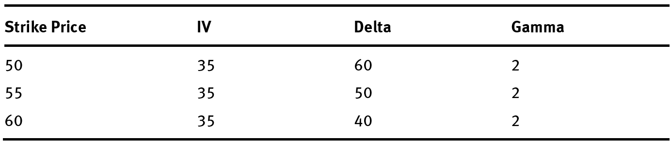
Volatility can act much like time. Running up IV can be like rolling the clock back. At the same time, low IV options have higher gamma than high IV options. If it sounds confusing, then now you understand why this is going to be the longest chapter of this book. Let’s start with the simple, low IV stocks versus high IV stocks. Stock XYZ is a low IV stock; its options (regardless of time to expiration) have deltas across strikes as shown in Figure 2.4. Based on delta levels, XYZ is assumed to be trading at or close to $55 at this point.

In the example in Figure 2.4, as the underlying moves from $55 to $60, the delta will go to from 50 to 35, a gamma of 3. Now let’s pump up the IV a touch in Figure 2.5.
An increase in IV makes all occurrences more likely, thus you’ll notice in Figure 2.5 that deltas have changed. The IV pump increased the deltas of the 50 and 60 strike options. This in turn causes the gamma of each strike to decrease. This is the way things work for ATM options and for options that have a long time to expire. But how does volatility affect OTM options?
Believe it or not, it was a student who taught me the best way to think about OTM options. The student pulled out a stream of options that looked like a normal curve. The normal curve represented delta; he then pulled the string just a bit. What I noticed was that near the peak (which is ATM) the slope decreased (change in slope of a delta curve is gamma). However, at the ends, where the student was actually pulling the strings, the slope increased. See the example of how gamma changes on an OTM call with an increase in volatility.
Take a look at the risk graph in Figure 2.6, notice the change in gamma with a 30% increase in volatility on an option with a delta of about 0.10 (we bought 20 contracts to make the move clear).

When an option is way out of the money, below a -0.15 delta, and up to a 0.15 delta, the options gamma will increase. Let’s look at some OTM options with an increase in IV in Figure 2.7 and Figure 2.8.
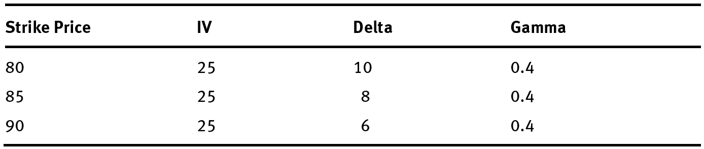
The options in Figure 2.7 represent options that are well out of the money. I am going to increase IV and then make up some deltas.

While it might seem insignificant, the gamma of the options above actually doubled from 0.4 to 0.8. This is the danger of shorting OTM options—the gamma can explode; I will go into detail later. Imagine that the above IV moves with an increase in the underlying. Imagine you are short the 85 calls and the underlying moves with a drop in volatility? Not only does the short delta change but the gamma increases. Now you know how someone can turn a small position into a loser of incredible proportions.
Vega
The vega of an option tracks how the option’s price moves with changes in implied volatility (IV). Think of it as the delta of implied volatility. If an option is worth 3.00 and has a vega of 1.00, and IV increases one point, the value of the option will be 4.00. Seems pretty simple—but it’s not. The nice thing about vega is that relative to gamma it is pretty simple . . . relative to gamma. In many ways, vega’s characteristics are exactly like the characteristics of delta; the big difference is that the Greek affected is the vega number (IV), not the delta number (underlying price).
Price of the Underlying
In simple terms, the higher the price of the underlying, the more vega it will have. SPX and SPY have essentially the same underlying, the S&P 500; but one represents the full value times 100. The other represents 1/10 of that value. As a result, SPX options have much more vega than SPY options. This is a result of each option being assigned to an underlying with much more value. An option on SPX can be worth 100 dollars or more. An increase in IV of 1 point might be at 5 dollars. That’s vega of 5. In SPY, an increase in IV in the same amount might only be 0.50. This means that SPX has vega of 5 and SPY has vega of 0.50. Compare XSP (mini SPX options) and SPX vegas on similar strikes and expirations in Figure 2.9.
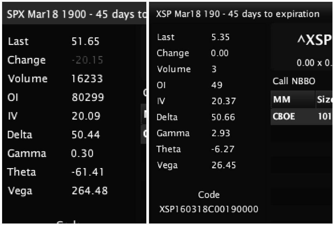
Note in the above, minus a decimal, the vega number would be exactly the same. This is clear evidence that it’s all about the price of the underlying when it comes to vega numbers.
Strike Price
The closer the strike price is to the money, the more vega it will have. The ATM options always have a high vega relative to the strikes that are out of the money. The further the strike moves from the underlying, the lower the vega. That doesn’t mean that managing vega is easy. Like gamma, vega can explode on a given strike price. The explosion of vega on a short strike, with the explosion of gamma, is what we in the business call a blowout—the complete inability for a trade to go forward because the clearing firm is forcing the trader to liquidate. The first rule of trading is that the trader must be able to trade the next day. If a trader blows out, he or she is likely in liquidation-only mode and will be out of a job or out of money. Either way, it’s an awful feeling and one that should be avoided at all costs.
Time to Expiration
One thing about volatility is that it does not move fluidly across the spectrum of expirations, sometimes called term structure. Options with a longer time to expire are worth more; they always will be. Thus, they have more vega.
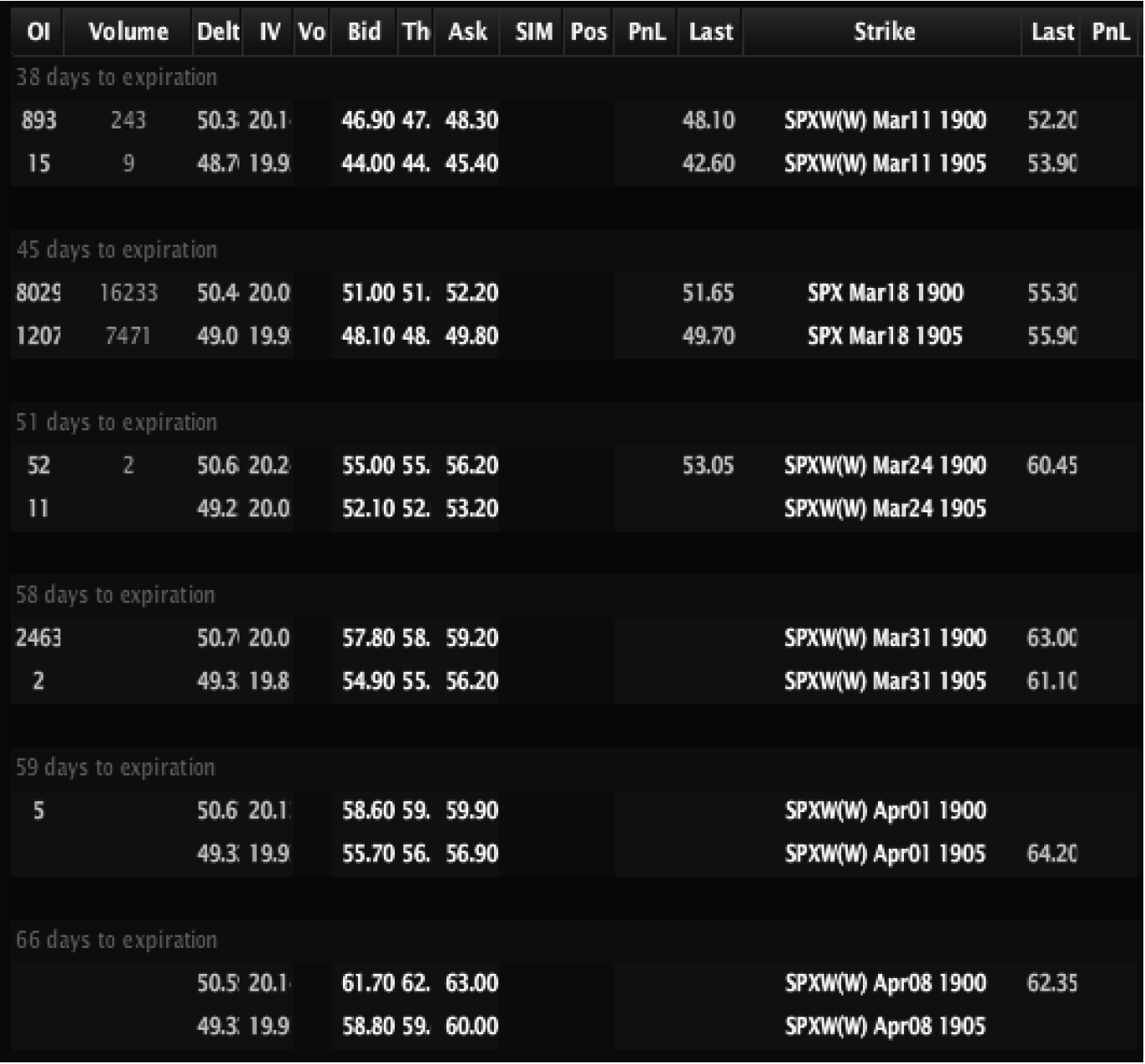
In the SPX options in Figure 2.10, the value of the ATM strike increases from about 47.50 up to 62.50 dollars from March to April when the options expire. That extra time premium, represents extra exposure to vega. If you have not made the connection by now, time premium equates to raw vega exposure.
The problem is that it doesn’t get any simpler from there. Just because an option has more vega does not mean it makes more money when IV explodes. That also doesn’t mean they move in the same manner as options with less time to expire. I am going to spend some time discussing this concept in detail later. However, to start let’s make one thing clear, an option with 1 month to expire and an option with 6 months to expire will have very different vegas, but the option with 1 month to expire will react to volatility in completely different ways.
If I own an asset that has movement at 25% and that movement increases to 30% near term, options will gain value, but the interpretation of a longer-term option will change too. A longer-term option will gain a much larger amount. This is because the market thinks that the underlying is going to keep moving the way it is moving now. Think about it this way: An option on an underlying for which vol increases from 25% to 30% will see its long-term options change in value, because the market assumes that movement has more increases still to come.
A jump in movement to 30%, even in the short term, must have a ramification on long term movement. If a stock starts flailing around, the long-term plays will pick up a lot of value, all else being equal. From a market-driven perspective, if people are scared, they do not just hedge their position for the next 30 days. Demand for positions in the underlying increases out 3, 6, and 12 months plus. All the way out to the longest LEAP, demand for shares is expected to increase. Banks and trading firms, those providing liquidity to hedgers, need to hedge trades they made with a lot of ‘edge’ in them that now maybe do not look so hot, this is the source of demand. Banks and trading firms need to follow rule number one (always be able to trade the next day), just like the individual trader. This creates demand in areas that are not being bought by the public, typically the back months.
Volatility
Strike prices that are ATM have the most vega. The further from ATM the strike price is, the less vega there will be. As IV increases, strike price characteristics become more alike. Thus, an increase in vol makes all options more like ATM, which have the most vega. As volatility increases for OTM strikes, they become more like ATM. Hence, volatility affects strike prices by making OTM options increase in vega until they become ATM options. As volatility increases, vega advances.
ATM options are quite simple; volatility can go wherever it wants; as long as it doesn’t go infinitely high, ATM vega will be stable.
Theta
Unlike delta, gamma, and to a lesser extent vega, there is no other Greek to tie theta to in terms of movement. Vega tends to move around based on time value, more or less. Theta is tied to gamma in terms of intensity, but not in terms of movement.
Theta is the rate at which an option loses value. Like all insurance products, as time passes an option loses a piece of value. If you buy an option in XYZ with a strike of $30 and pay 3 ($300), and the underlying is trading at $29 per share, if the underlying still trades at $29 at expiration, that option must be worth zero. The process of that option getting to zero, in the days that passed, is what theta measures.
Price of the Underlying
Much like vega, when an underlying is high, options will have a high theta. Going back to our XSP and SPX example, the same thing that produces a higher vega in options produces a higher theta. In Figures 2.11 and 2.12 you can see that an OTM option in SPX relative to XSP is going to be worth about 10 times that of an XSP option.

Over the next 45 days, the SPX option has 10 times the dollar value to lose. Having 10 times the value means that over the next 45 days instead of losing 5 dollars, the option has to lose 50. Thus, ceteris paribus, the higher the price, the higher the theta.
Strike Price
ATM options have the highest premium. These have the highest theta number. In addition, ATM options have the standard theta curve, Figure 2.13, that we are all used to seeing:
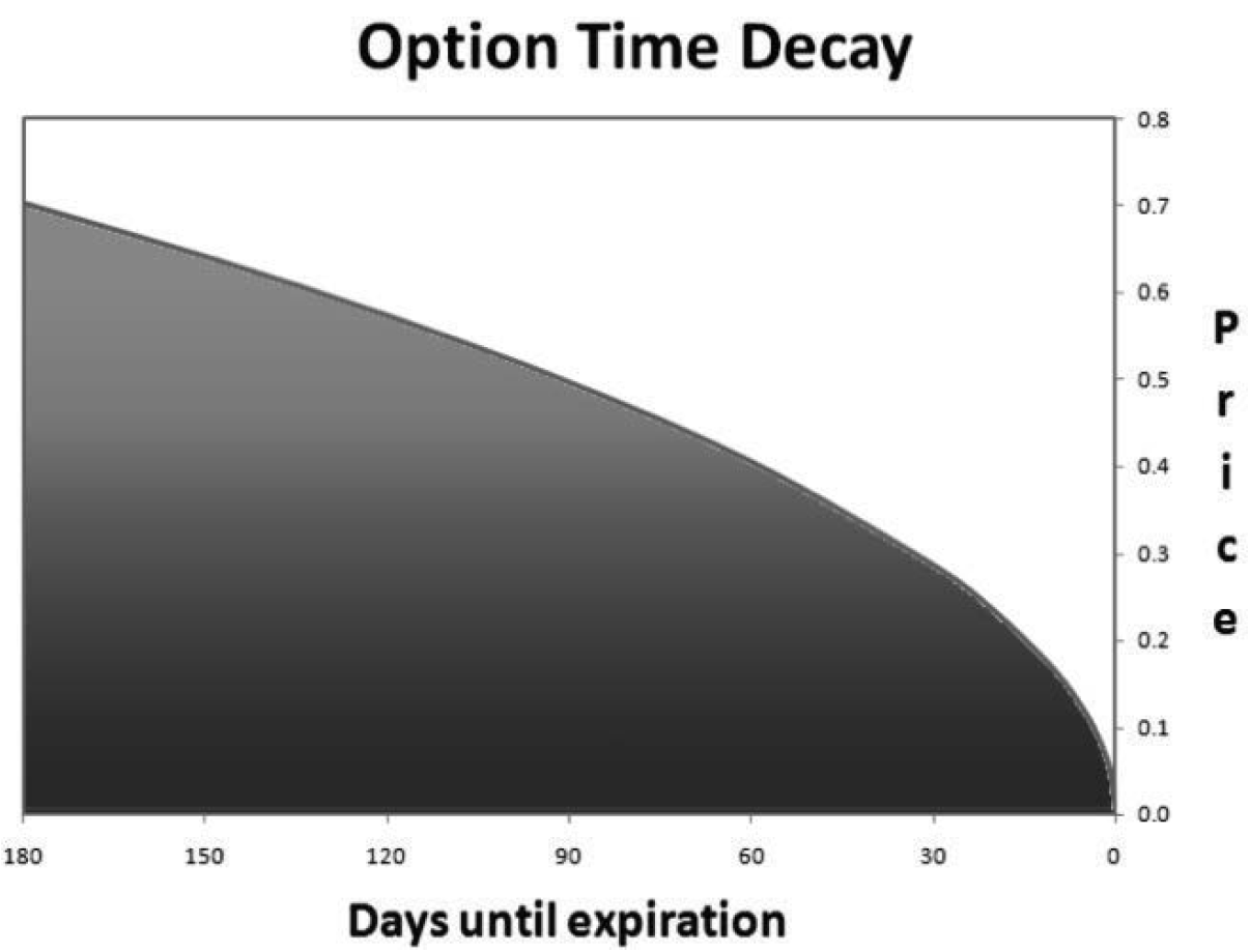
As time to expiration approaches, ATM options see their theta increase exponentially. With the 30 days having huge theta, and the final 7 days having massive theta getting even higher.
OTM options are not the same. The decay curve for OTM options is much more linear than that of ATM options. As strike becomes more and more OTM, the theta decay becomes more linear. Decay is more linear the further out of the money an option is.
Unit options are options worth very little and far out of the money. For a standard stock, I would expect that a unit option will be worth less than .15 or so. These are options that have no value other than pure catastrophe insurance and they take forever to decay. There are two main reasons that these options retain value:
1.Margining: Market makers have their margin assessed in two ways. The more margin market makers have, the more capital is tied up. So, if market makers are trying to be as capital efficient as possible, they will always stay away from selling options that tie up margin by a large amount.
The SEC mandates that for every option, be it worth .05 or 5,000, the market maker is charged at least .25 per contract. An option worth .05 ties up an inordinate amount of margin for the market maker. If I am short one hundred 5 cent options, I can make 500.00 (.05 * 100 * 100) on the 100 options I am short. At the minimum, even if I am long, I am going to be charged $25 of margin due to SEC rules. That may not be the best engagement of capital.
The more treacherous effect on margin is risk haircut. Clearing firms run an algorithm on a portfolio assessing risk if the underlying moves 10, 20, and up to 40%. A trader who has several of these short option positions can see the cost of owning a position via ‘tinnie options’ go much higher as .05 options are seen as a serious risk (back in the day ‘tinnie options’ were described as options worth 1/16 of a dollar or less, now usually they are referred to as options worth less than .10). Additionally, they run risk on increases in volatility of up to 400%. The charge of margin on these options can be astronomically high. If a trader is short 100 .05 options and IV increases 400%, suddenly the ‘worthless’ out of the money options that were sold at .05 are no longer worthless. Seeing this, the clearing firm must raise the margin requirements by a large amount. Clearing firms, understanding the risk potential, do not wait for vega to explode; they margin some of this risk into the options from day one. This makes being short these options potentially as expensive as the premium collected. Putting up large amounts of capital to make $500 is not what traders typically try to accomplish. Being short cheap options is not an efficient use of capital. This is going to slow the rate of decay in ways that the option pricing model cannot measure.
2.The actual risk reward is the other issue with units. If you are a bottomless pit of money, you expect the value of shorting an option worth .05 to be high; they often end up worthless. However, most traders are not bottomless pits of money. The ability to make $500 on a $100 lot that is 99% likely to win, does not counteract the risk of loss, say $25,000 once, even if it has a positive expectation. Major firms don’t care about these type of losses, but the average retail trader does.
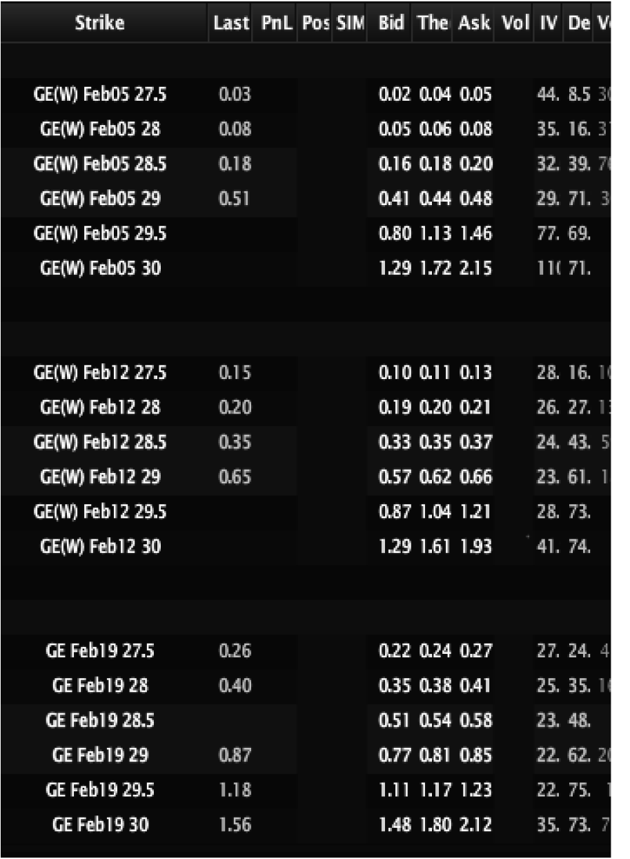
When I was interviewing candidates at Group One Trading, we asked college kids if they would risk 500,000 dollars on a coin flip if they could win 1 million dollars if they were right. If they said yes, they were unlikely to get a job. We simply did not have that kind of risk appetite; neither do most market making firms, except those with the deepest pockets. The ‘risk appetite’ effect on small options keeps them bid higher for longer. This slows the decay in these options beyond what the pricing model expects. Based on values in GE (General Electric) options in Figure 2.14, the 27.5 puts lost more value between week 3 and week 2 then they did from week 2 to week 1. This is the ‘unit effect,’ the idea that once an option hits a specific value its rate of decay breaks from the pricing model and slows to a crawl. Once an option hits its unit effect level, the cost of being short tends to become a bad trade for the average trader.
Time to Expiration
In general, the further the time to expiration, the greater the need for insurance. The insurance decay slows down, especially for options that are near the money. The longer to expiration, the slower the decay. If you look at delta decay instead of strike decay, the story changes.
I just got done explaining that at the strike level, the further away from ATM, the more linear the decay. However, if I follow option delta decay, how a portfolio that is constantly holding a 0.20 delta option, regardless of what option that is, decays, the story changes. The decay of the 0.20 delta option is in fact exponential. Thus the 0.20 delta option at 2 years will decay more slowly than the 0.20 delta option at 1 year, which will decay much more slowly than the 0.20 delta option at 6 months, and so on.
This means that while you might be used to options decaying a certain way, at 10% out of the money or 20% out of the money, if we follow the decay of options with 0.10 delta at 2 years to expiration and then follow the decay on trading opportunities rolling down to delta, there may be an opportunity to take advantage of theta. Option decay from a delta perspective follows a similar path to ATM options, being short a 0.20 delta option on a constant basis will produce a curve very similar to that of an ATM option.
To sum things up, theta burn following deltas is exponential, but following percentages out of the money is more linear.