Historical Volatility (HV)

Historical volatility is a backward-looking number. It is a representation of the history of volatility. Historical volatility typically uses a calculation called GARCH (Generalized Autoregressive Conditional Heteroskedasticity) to calculate how much an instrument has moved over a previous period of days. Without getting too deep into the weeds, the GARCH model compares where the underlying closed the previous day relative to where it closed the next day and determines how much the underlying moved. HV uses a set number of days in the GARCH model to calculate volatility over previous days.

GARCH is limited by one major flaw: it only looks at end-of-day pricing. It misses how much an underlying might move throughout the day. If the S&P 500 moves UP 15 points and then down 20 and settles the day up 5, GARCH modelling will only see 5 points of movement. Is that 5 points of movement an accurate way of portraying how much the underlying moved? The answer is no, so while HV is important, it doesn’t tell the whole story.

Even so, historical volatility is what tends to drive price perceptions going forward. The assumption is that how volatility moved in the past will be a good indicator of how volatility will move in the future. In betting on how something will move, we tend to look at specific time periods, each meaning different things depending on the amount of data reviewed.

Short-Term Historical Volatility

Short-term HV studies periods existing over less than a month. This means looking at the last 10 trading days, the last 20 trading days, and the last 30 trading days. Figure A.1 shows a graph of the volatility over time.

Figure A.1: Short-term Historical Volatility.

HV10 moves much more quickly than 20 day volatility and HV20 moves more than 30 day, although the difference in movement between 20 and 30 is far less than the difference in movement between 10 and 20. Near-dated HV gives you a view of what has happened recently. It tends to miss some intra-day movement. It also tends to be the best view of what might happen next. These should be looked at in three month increments at most.

Intermediate-Term Historical Volatility

If near-dated HV gives you a view of what has been going on recently and what might happen next, intermediate HV is going to give you the general trend of movement based on the last 2–6 months. High volatility tends to lead to more volatility and low volatility tends to lead to lower volatility. Looking at intermediate volatility gives you an idea of what the general trend has been on the product over the last few months. It tends to be smoother, but can still anticipate major movement.

A vol trend frees you from some of the noise of near-dated HV. When this hits historic levels, it can mean that the underlying is at a reversal point. Be wary when these numbers are hitting highs or lows, because that can mean the market is setting a trap and is primed for a reversal. In Figure A.2, SPX movement is below 7% over the previous 60 days and below 8% over the previous 90 days, about as low as movement in the S&P 500 will get. I find this type of information invaluable as it helps me see that movement is lacking, at a minimum will not go much lower, and is likely to go higher. When I view movement at historic lows, I know that even if I don’t want to buy options, I also do not want to be net short options.

Figure A.2: Intermediate-Term Historical Volatility (HV of 60 and 90 days).

Long-Term Historical Volatility

Long-term HV is meant to point out where the mean reversion point is. Movement is always mean reverting to a point. If movement has been steadily decreasing, as it was in Figure A.2, and mean reversion is in the cards, long-term HV is where you will see the movement unless the underlying is completely breaking out. This reversion level, like a stock’s moving average, is dynamic and will act like a resistance point. Consider long-term HV to be a reversion level for the underlying.

180 day vol, shown in the lower graph in Figure A.3, acts as a near term stop for movement and tends to be a resistance point for forward-looking volatility measures. In Figure A.3, the 180 vol is about 11%, pointing toward where near term vol is likely to find resistance if HV increases from the 6% it was trading. 360-day HV can show the true reversion level if an event occurs or movement starts to increase. Yes, the underlying IV might explode higher but, in general, when other vol measures hit HV360 that will be a level where price either goes much higher or turns around.

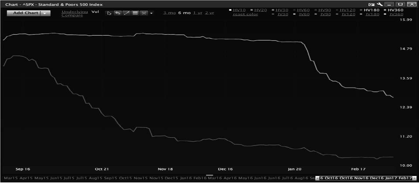
Figure A.3: Long-Term Historical Volatility.

Realized Volatility (RV)

Realized volatility is how the underlying is moving at the moment. This term describes how an underlying moved while you are setting up a trade. It can also be interchangeable with short-term HV. You look at what amounts to HV of 10 to 20 days. For the most part, when I think about realized volatility, I think about 10 day HV.

Looking at Figure A.4, which is 10 day HV, I can describe how the S&P 500 (SPX) has been moving in the recent past, which is the best I can do to describe what is happening right now. While HV10 can say what’s happened in the recent past, it can’t say what is actually happening right now. This is the one place where something like candlesticks might actually show movement. The candlestick, the pattern seen on most modern charts, shows a great deal of information: High to low (the rectangular ‘real body’), trading range extension above and below, and direction (white candles moved up, black candles moved down).

Figure A.4: Realized 10-Day Volatility.

I can see ups and downs on this candlestick chart (Figure A.5). Combined with historical analysis, you can see what is going on with the underlying instrument. In the chart above, in my eyes, the answer is a trend. SPX has slow momentum higher.

Figure A.5: Candlestick chart.

Forward Volatility

Forward volatility is how much an asset might move going forward over a certain period of time. The options pricing model uses five factors: (1) underlying price, (2) strike price, (3) time to expiration, (4) cost of carry, and (4) forward volatility.

The problem is that no one knows what forward volatility will be. This is what creates option trading opportunities. In this book, you have seen how the ignorance of forward volatility is where all of the trading uncertainty exists. Understanding that forward vol is a moving target allows you to make profitable trades. If forward vol were known, there would be no trading.

Implied Volatility (IV)

Implied volatility is the market’s best guess at how volatility will be going forward. While HV is backward facing, IV is forward facing. IV does rely on the past, but it also takes into account what might happen in the future. What is interesting, and a common misconception, is that IV is actually an output of the pricing model, not an input.

The pricing model is based on the Black-Scholes formula, used for calculating what an option’s price should be in theory. While an older model, it is the source for many newer models. Traders use many types of pricing models, but all options models use the following five factors: (1) price of the underlying, (2) strike price of the option, (3) time to expiration of the option, (4) cost of carry, and (5) forward volatility that was originally used in the model developed in Black-Scholes.

This sounds easy, except that we only know four of the five factors. We do not know what forward volatility is going to be. Thus was born implied volatility. IV is derived using what we know: the four factors in the pricing model. Using the options price and the four factors, we run a formula to solve for forward volatility via calculus, creating implied volatility. Implied volatility is an output of the pricing model, not an input. Thus, as the factors of the model change or the option’s price changes, IV changes. The Greeks are based on IV and can also move based on what happens with the four factors and the option’s price. IV is a market-driven number. Here is an example of how that equation for IV looks:

Option Price = Stock Price*Time*Carry*Strike*X Unknown Forward Volatility (IV)

If a $30 stock has an ATM options price of 2.00 with 30 days to expire, a carrying cost of 0.05, and a strike of 30, the formula would be at onset:

2.00=30*30*0.05*30*X

When the market moves IV to an extreme, there is a chance to set up a trade. It depends on whether you think options are fairly priced. IV as seen in VIX moves up and down much like a stock price as shown if Figure A.6.

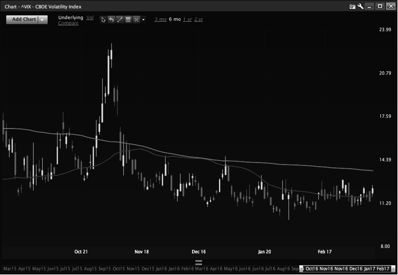
Figure A.6: IV movement.

The only difference between HV and IV is that IV is driven by concepts of mean reversion—the assumption that volatility returns to a mean.

Calls and Puts

An option is a contract that enables you to buy or sell an underlying or an asset at a specific price and time. An option that allows you to buy at a pre-determined price is called a call. A call option is exercised only when the strike price is below the market price of the underlying, without exception. A put is the opposite. An option that gives the owner the right to sell at a specific price is referred to as a put. A put would be exercised if the strike price is above the market price of the underlying (in the money), without exception.

Skew

Skew is the relationship between puts and calls as they relate ATM (at the money). It is the formation of volatilities of options below the current price, relative to at-the-money options, relative to options that are above the strike. OTM options trade relative to ATM options’ skew. Options are not tied to one another, but they are connected. When ATM IV moves, calls and puts move, but not necessarily at the same rate. When IV falls, the same is true. OTM calls and OTM puts can move free of ATM options. An out-of-the-money call and an out-of-the-money put can gain value whether the ATM options values change or not, especially in indexes and ETFs if a customer that has an axe to grind on a particular option, portion of the curve, or direction of the underlying. Take a look at the skew chart in Figure A.7.

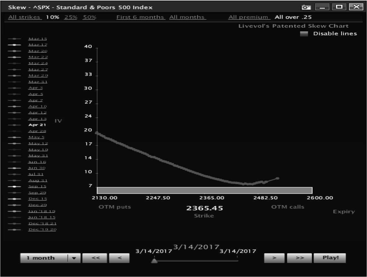
Figure A.7: Skew chart.

SPX, like most indexes, has a higher IV for puts than for calls. However, this curve doesn’t remain constant, but moves with changes in the underlying price and also with trade volume in options. While it is hard to see, there are spots where vol is cheap or expensive in relative terms. The dots line up around the 2250 strike in Figure A.7.

Skew can get out of whack. Look at FEZ, a leveraged ETF 2X long on the Eurozone (Figure A.8). The 35 calls are cheaper than the 39 calls even though the 39 calls are OTM. What drove this? Customer call buying. A customer bought 20,000 of the 39 calls in FEZ ahead of this vol set-up.

Here is how to judge skew:

Figure A.8: Skew chart 2.

Looking at the curve above in Figure A.8, we can see where skew went out of whack. In FEZ the 30 puts were more expensive than the 31 or 32 puts. There was likely an order driving up volatility in the May 30 puts. This type of action needs to be evaluated so that you know what is going on, and can potentially find price ranges where you can make money.

Term Structure

While volatility is often presented as a single concept, it is not. Volatility does not move evenly across every contract. While all volatility is correlated, it is not tied at the hip. As skew is created by different demand for different strikes, term structure is created by demand for options in different months.

Implied volatility is created by demand; so just as demand is not going to be the same for a given strike, demand will also not be even across different months. In equities, there will be more demand for options during earnings months or when the stock has an important announcement coming. Look at AAPL term structure (Figure A.9). Earnings were predicted as coming up in the term structure below.

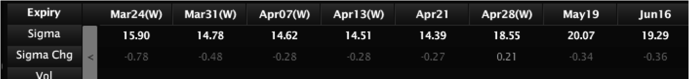
Figure A.9: Predicting earnings with term structure.

Based on Figure A.9 above, earnings were unlikely to be announced before April 21st. Less certain was whether earnings would be published after the April 28th contract or sometime before May expire. Earnings before the May contract expire create one scenario; and the April 28 contract had a dramatic increase in IV over April 13. May was higher than the April 28th contract and June showed lower IV than May. This can also be observed in pharmaceutical stocks that have drugs up for FDA review. You can see when the market thinks an FDA decision might occur.

When I was a floor trader, I traded a stock called Sepracor. The company was developing a sleep aid called Lunesta. The FDA committee approval was a moving target; thus, term structure was constantly changing. When it appeared something was imminent, IV would pop, and when that turned out to be nothing, IV would tank. However, the official FDA approval date never moved, it was always a contract that customers wanted to own. I managed the fact that traders wanted to sell me the ‘boring months’ to buy the ‘action months.’

Volatility between months is related, not tied. Order flow (customer demand) can drive one month in a different direction than another. This is just the way equity flow runs. Index flow is a touch different but can share similar characteristics.

Index term structure is often driven by events. Take a look at Figure A.10, the S&P 500 a few months before the time of Brexit.

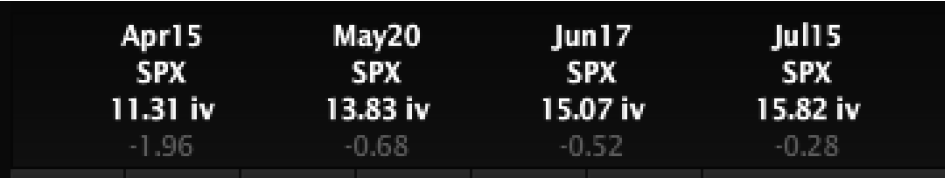
Figure A.10: S&P 500 pre-Brexit.

Even in April the market was pricing some type of event to happen in June or July. That turned out to be the Brexit.

Term structure provides a ton of information:

Used to the trader’s advantage, you may be able to develop a trade you think will make money.

Term structure is valuable and crucial in developing calendar spreads, for example. When a month seems mispriced, you can use term structure to develop a trade.

Volatility Index (VIX)

The VIX is the CBOE Volatility index. The VIX represents the calculated value of volatility in SPX options (options on the S&P 500) that expire in 30 days. How does it do this? It’s complicated.

The VIX Index looks at the weekly options expiring on the Friday before and after a 30-day time horizon in the SPX and pulls implied volatility from every strike with a bid (traders are at least willing to pay 0.05 for the option). The index is called the “fear gauge” or “fear index,” and tends to have a negative correlation to the S&P 500. When the SPX is up, the VIX tends to be down. When the SPX is down, the VIX tends to be up.

We do not like the description of VIX as a fear gauge. We prefer to call it the insurance gauge. The VIX measures how much it costs to insure a portfolio. When the VIX is high, it points to market turmoil. Look at a chart of VIX in Figure A.11.

Figure A.11: VIX chart.

When VIX was high, markets were a mess. VIX tends to move before a major event. In the case of Brexit, VIX started to rally two weeks before the vote. It did the same thing ahead of the 2016 presidential election in the U.S.

The VIX index is the baseline for setting volatility across any product that is traded in the equity space. If VIX is low, vol in that equity should lean lower. If it doesn’t, that could be a trade.

Delta

Delta is slope. It represents your exposure to directional movement in the underlying stock. If a position expects the underlying to rally, it positively correlates with the underlying. If the position expects the underlying to fall, the position is short delta. An example:

A position is long 100 delta. If the underlying rallies 1 point, the position will make 100.00 (1*100). If the underlying falls one point, the position will lose 100.00 (–1*100).

A position is short 100 delta. If the underlying rallies 1 point, the positions will lose 100 (1*–100). If the underlying falls one point, the position will make 100 (–1*–100).

Delta is directional exposure. If a position will make or lose money based on movement on the underlying, the position has delta. Look at a chart of a long call. With a 0% move, the contract has no P&L, but for every 2% move it picks up about its delta in P&L.

Delta is the red line in Figure A.12. As the underlying rallied in a direction, how does the position perform?

Figure A.12: Delta chart.

Gamma

When you have a position as the underlying moves around, you will see delta change—this degree of change is gamma. Gamma is a position’s exposure to movement, not in one particular direction, rather movement in either direction. Look at a chart of 20HV in the SPX in Figure A.13.

Figure A.13: 20 day HV in SPX.

This movement shows where gamma comes into play. When the SPX starts to move, it measures gamma as a related factor. That occurs often.

A common problem among traders is understanding that the sign of gamma has nothing to do with the sign of delta. You can have a positive gamma and negative delta and vice versa. What gamma measures is what happens to delta as the underlying moves. If you are short delta and long gamma and the underlying rallies, you become less short delta. If you are short delta and long gamma and the underlying falls, you will become more short delta with exposure to the underlying.

Gamma doesn’t directly affect P&L; it affects delta. Following are some examples of the math behind gamma:

Look at the call from above. Delta changes as the underlying rallies in Figure A.14.

Figure A.14: Delta changes.

At a 0% move, delta was 49. When SPY was up 2%, delta changed to 84. That is the way gamma helps you measure and manage trades. A quick increase in the underlying dramatically changes delta, and that change is gamma.

Theta

Theta represents the position’s exposure to time. As a day passes, the theta of a position tells you whether or not you are making money. If a position has theta of positive 100 and a day passes, the position should in theory make $100.00. Look at a chart of option premiums on a long call option in Figure A.15.

Figure A.15: Multiple payouts in SPX over the life of a call option.

As time passes, ATM options move. The way to measure that cost is theta. Options are like insurance—as time passes, insurance policies lose value, and the loss of insurance value is what theta measures. It works in your favor if you are short premium, and against you when you are long. Think about theta like this:

Theta is what the position produces in time decay, which is not an easy thing to keep track of over multiple positions and many option trades—unless you manage positions with theta in mind.

Vega

Vega is to volatility as delta is to underlying price. When IV increases, vega reacts to the movement in implied volatility. A one point increase in implied volatility will cause the option position to gain the value of its vega. Look at a chart of the call above with a change in implied volatility in Figure A.16.

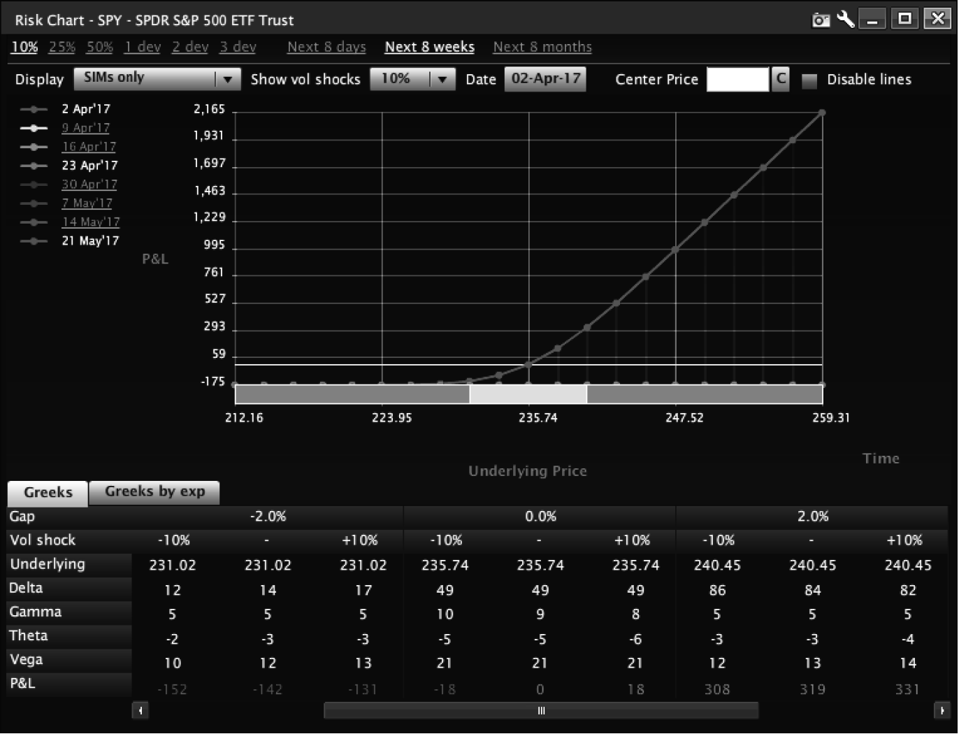
Figure A.16: A call payout in SPX.

If IV rallies 10%, the position makes money. This is directly related to the vega of the position. Negative vega will behave the opposite of the above and is created by short options. Vega, like gamma, moves less as the underlying moves away from the starting price of the trade.